
1
Machine Learning and Financial Engineering
Wavelet networks are a new class of networks that combine the classic sigmoid neural networks and wavelet analysis. Wavelet networks were proposed by Zhang and Benveniste (1992) as an alternative to feedforward neural networks which would alleviate the weaknesses associated with wavelet analysis and neural networks while preserving the advantages of each method.
Recently, wavelet networks have gained a lot of attention and have been used with great success in a wide range of applications, ranging from engineering; control; financial modeling; short-term load forecasting; time-series prediction; signal classification and compression; signal denoising; static, dynamic, and nonlinear modeling; to nonlinear static function approximation.
Wavelet networks are a generalization of radial basis function networks (RBFNs). Wavelet networks are hidden layer networks that use a wavelet for activation instead of the classic sigmoidal family. It is important to mention here that multidimensional wavelets preserve the “universal approximation” property that characterizes neural networks. The nodes (or wavelons) of wavelet networks are wavelet coefficients of the function expansion that have a significant value. In Bernard et al. (1998), various reasons were presented for why wavelets should be used instead of other transfer functions. In particular, first, wavelets have high compression abilities, and second, computing the value at a single point or updating a function estimate from a new local measure involves only a small subset of coefficients.
In statistical terms, wavelet networks are nonlinear nonparametric estimators. Moreover, the universal approximation property states that wavelet networks can approximate, to any degree of accuracy, any nonlinear function and its derivatives. The useful properties of wavelet networks make them an excellent nonlinear estimator for modeling, interpreting, and forecasting complex financial problems and phenomena when only speculation is available regarding the underlying mechanism that generates possible observations.
In the context of a globalized economy, companies that offer financial services try to establish and maintain their competitiveness. To do so, they develop and apply advanced quantitative methodologies. Neural networks represent a new and exciting technology with a wide range of potential financial applications, ranging from simple tasks of assessing credit risk to strategic portfolio management. The fact that neural and wavelet networks avoid a priori assumptions about the evolution in time of the various financial variables makes them a valuable tool.
The purpose of this book is to present a step-by-step guide for model identification of wavelet networks. A generally accepted framework for applying wavelet networks is missing from the literature. In this book we present a complete statistical model identification framework to utilize wavelet networks in various applications. More precisely, wavelet networks are utilized for time-series prediction, construction of confidence and prediction intervals, classification and modeling, and forecasting of chaotic time series in the context of financial engineering. Although our proposed framework is examined primarily for its use in financial applications, it is not limited to finance. It is clear that it can be adopted and used in any discipline in the context of modeling any nonlinear problem or function.
The basic introductory notions are presented below. Fist, financial engineering and its relationship to machine learning and wavelet networks are discussed. Next, research areas related to financial engineering and its function and applications are presented. The basic notions of wavelet analysis and of neural and wavelet networks are also presented. More precisely, the basic mathematical notions that will be needed in later chapters are presented briefly. Also, applications of wavelet networks in finance are presented. Finally, the basic aspects of the framework proposed for the construction of optimal wavelet networks are discussed. More precisely, model selection, variable selection, and model adequacy testing stages are introduced.
Financial Engineering
The most comprehensive definition of financial engineering is the following: Financial engineering involves the design, development, and implementation of innovative financial instruments and processes, and the formulation of creative solutions to problems of finance (Finnerty, 1988). From the definition it is clear that financial engineering is linked to innovation. A general definition of financial innovation includes not only the creation of new types of financial instruments, but the development and evolution of new financial institutions (Mason et al., 1995). Financial innovation is the driving force behind the financial system in fulfilling its primary function: the most efficient possible allocation of financial resources (Ζαπράνης, 2005). Investors, organizations, and companies in the financial sector benefit from financial innovation. These benefits are reflected in lower funding costs, improved yields, better management of various risks, and effective operation within changing regulations.
In recent decades the use of mathematical techniques and processes, derived from operational research, has increased significantly. These methods are used in various aspects of financial engineering. Methods such as decision analysis, statistical estimation, simulation, stochastic processes, optimization, decision support systems, neural networks, wavelet networks, and machine learning in general have become indispensable in several domains of financial operations (Mulvey et al., 1997).
According to Marshall and Bansal (1992), many factors have contributed to the development of financial engineering, including technological advances, globalization of financial markets, increased competition, changing regulations, the increasing ability to solve complex financial models, and the increased volatility of financial markets. For example, the operation of the derivatives markets and risk management systems is supported decisively by continuous advances in the theory of the valuation of derivatives and their use in hedging financial risks. In addition, the continuous increase in computational power while its cost is being reduced makes it possible to monitor thousands of market positions in real time to take advantage of short-term anomalies in the market.
In addition to their knowledge of economic and financial theory, financial engineers are required to possess the quantitative and technical skills necessary to implement engineering methods to solve financial problems. Financial engineering is a unique field of finance that does not necessarily focus on people with advanced technical backgrounds who wish to move into the financial area but, is addressed to those who wish to get involved in investment banking, investment management, or risk management.
There is a mistaken point of view that financial engineering is accessible only by people who have a strong mathematical and technical background. The usefulness of a financial innovation should be measured on the basis of its effect on the efficiency of the financial system, not on the degree of novelty that introduces. Similarly, the power of financial engineering should not be considered in the light of the complexity of the models that are used but from the additional administrative and financial flexibility that it offers its users. Hence, financial engineering is addressed to a large audience and should be considered within the broader context of the administrative decision-making system that it supports.
Financial Engineering and Related Research Areas
Financial engineering is a very large multidisciplinary field of research. As a result, researchers are often focused on smaller subfields of financial engineering. There are two main branches of financial engineering: quantitative finance and financial econometrics. Quantitative finance is a combination of two very important and popular subfields of finance: mathematical finance and computational finance. On the other hand, financial econometrics arises from financial economics. Research areas related to financial engineering are illustrated in Figure 1.1.
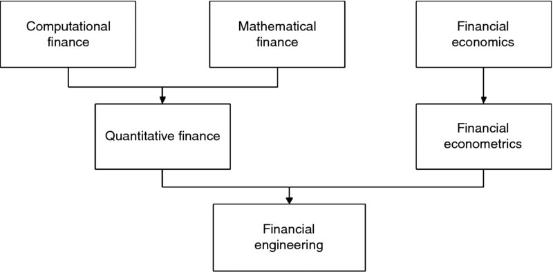
Figure 1.1 Research areas related to financial engineering.
The scientific field of financial engineering is closely related to the relevant disciplinary areas of mathematical finance and computational finance, as all focus on the use of mathematics, algorithms, and computers to solve financial problems. It can be said that financial engineering is a multidisciplinary field involving financial theory, the methods of engineering, the tools of mathematics, and the practice of programming. However, financial engineering is focused on applications, whereas mathematical finance has a more theoretical perspective.
Mathematical finance, a field of applied mathematics concerned with financial markets, began in the 1970s. Its primary focus was the study of mathematics applied to financial concerns. Today, mathematical finance is an established and very important autonomous field of knowledge. In general, financial mathematicians study a problem and try to derive a mathematical or numerical model by observing the output values: for example, market prices. Their analysis does not necessarily have a link back to financial theory. More precisely, mathematical consistency is required, but not necessarily compatibility with economic theory.
Mathematical finance is closely related to computational finance. More precisely, the two fields overlap. Mathematical finance deals with the development of financial models, and computational finance is concerned with their application in practice. Computational finance emphasizes practical numerical methods rather than mathematical proofs, and focuses on techniques that apply directly to economic analyses. In addition to a good knowledge of financial theory, the background of people working in the field of computational finance combines fluency in fields such as algorithms, networks, databases, and programming languages (e.g., C/C++, Java, Fortran).
Today, the disciplinary area of mathematical finance and computational finance constitutes part of a larger, established, and more general area of finance called quantitative finance. In general, there are two main areas in which advanced mathematical and computational techniques are used in finance. One tries to derive mathematical formulas for the prices of derivatives, the other one deals with risk and portfolio management.
Financial econometrics is another field of knowledge closely related (although more remote) to financial engineering. Financial econometrics is the basic method of inference in the branch of economics termed financial economics. More precisely, the focus is on decisions made under uncertainty in the context of portfolio management and their implications to the valuation of securities (Huang and Litzenberger, 1988). The objective is to analyze financial models empirically under the assumption of uncertainty in the decisions of investors and hence in market prices. For example, the martingale model for capital asset pricing is related to mathematical finance. However, the empirical analysis of the behavior of the autocorrelation coefficient of the price changes generated by the martingale model is the subject of financial econometrics.
We illustrate the various subfields of financial engineering by the following example. A financial economist studies the structural reasons that a company may have a certain share price. A financial mathematician, on the other hand, takes the share price as a given and may use a stochastic model in an attempt to derive the corresponding price of a derivative with the stock as an underlying asset. The fundamental theorem of arbitrage-free pricing is one of the key theorems in mathematical finance, while the differential Black–Scholes–Merton approach (Black and Scholes, 1973) finds applications in the context of pricing options. However, to apply the stochastic model, a computational translation of the mathematics to a computing and numerical environment is necessary.
Functions of Financial Engineering
Financial engineers are involved in many important functions in a financial institution. According to Mulvey et al. (1997), financial engineering is used widely in four major functions in finance: (1) corporate finance, (2) trading, (3) investment management, and (4) risk management (Figure 1.2). In corporate finance, large-scale businesses are interested in raising funds for their operation. Financial engineers develop new instruments or enhance existing ones in order to secure these funds. Also, they are involved in takeovers and buyouts. In trading of securities or derivatives, the objective of a financial engineer is to develop new dynamic trading strategies. In investment management the aim is to develop new investment vehicles for investors.
Examples presented by Mulvey et al. (1997) include high-yield mutual funds, money market funds, and the repo market. In addition, they develop systems for transforming high-risk investment instruments to low-risk instruments by applying techniques such as repackaging and overcollaterization. Finally, in risk management, a financial engineer must, on the one hand, assess the various types of risk of a range of securities and, on the other hand, use the appropriate methodologies and tools to construct portfolios with the desired levels of risk and return. These methodological approaches relate primarily to portfolio insurance, portfolio immunization against changes in certain financial variables, hedging, and efficient assets/liability management.
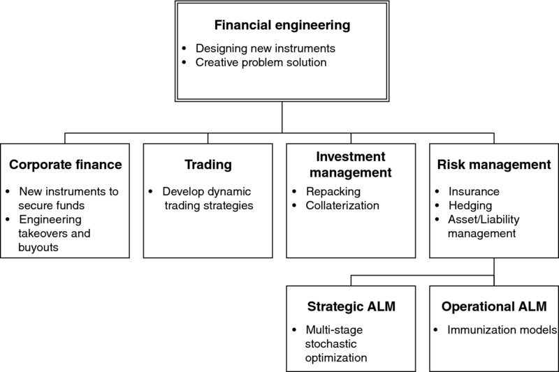
Figure 1.2 Financial engineering activities according to Mulvey et al. (1997).
Risk management is a crucial part of corporate financial management. The interrelated areas of risk management and financial engineering find direct applications in many problems of corporate financial management, such as assessment of default risk, credit risk, portfolio selection and management, sovereign and country risk, and financial programing, to name a few.
During the past three decades, a series of new scientific tools derived from the wider field of operations research and artificial intelligence has been developed for the most realistic and comprehensive management of financial risks. Techniques that have been proposed and implemented include multicriteria decision analysis, expert systems, neural networks, genetic and evolutionary algorithms, fuzzy networks, and wavelet networks. A typical example is the use of neural networks by Zapranis and Sivridis (2003) to estimate the speed of inversion within the Vasicek model, used to derive the term structure of short-term interest rates.
Applications of Machine Learning in Finance
Neural networks and machine learning in general are employed with considerable success in primarily three types of applications in finance: (1) modeling for classification and prediction, (2) associative memory, and (3) clustering (Hawley et al., 1990). The use of wavelet networks is shown in Figure 1.3.
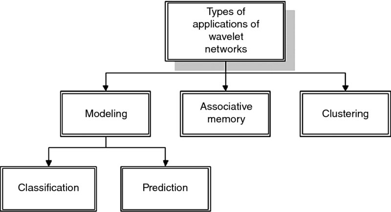
Figure 1.3 Types of applications of wavelet networks.
Classification includes assignment of units in predefined groups or classes, based on the discovery of regularities that exist in the sample. Generally, nonlinear nonparametric predictors such as wavelet networks are able to classify the units correctly even if the sample is incomplete or additional noise has been added. Typical examples of such applications are the visual recognition of handwritten characters and the identification of underwater targets by sonar. In finance, an example of a classification application could be the grouping of bonds, based on regularities in financial data of the issuer, into categories corresponding to the rating assigned by a specialized company. Other examples are the approval of credit granting (the decision as to who receives credit and how much), stock selection (classification based on the anticipated yield), and automated trading systems.
The term prediction refers to the development of mathematical relationships between the input variables of the wavelet network and usually one (although it can be more) output variable. Artificial networks expand the common techniques that are used in finance, such as linear and polynomial regression and autoregressive moving averages (ARMA and ARIMA). In finance, machine learning is used mainly in classification and prediction applications. When a wavelet network is trained, it can be used for the prediction of a financial time series. For example, a wavelet network can be used to produce point estimates of the future prices or returns of a particular stock or index. However, financial analysts are usually also interested in confidence and prediction intervals. For example, if the price of a stock moves outside the prediction interval, a financial analyst can adjust the trading strategy.
In associative memory applications the goal is to produce an output corresponding to the class or group desired, based on one input vector presented in the neural network that determines which output is to be produced. For example, the input vector may be a digitized image of a fingerprint, and the output desired may be reconstruction of the entire fingerprint.
Clustering is used to group a large number of different input variables, each of which, however, has some similarities with other inputs. Clustering is useful for compression or filtering of data without the loss of a substantial part of the information. A financial application could be the creation of clusters of corporate bonds that correspond to uniform risk classes based on data from financial statements. The number and composition of the classes will be determined by the model, not by the user. In this case, in contrast to the use of classification, the categories are not predetermined. This method could provide an investor with a diversified portfolio.
From Neural to Wavelet Networks
In this section the basic notions of wavelet analysis, neural networks, and wavelet networks are presented. Our purpose is to present the basic mathematical and theoretical background that is used in subsequent chapters. Also, the reasons that motivated the combination of wavelet analysis and neural networks to create a new tool, wavelet networks, are discussed.
Wavelet Analysis
Wavelet analysis is a mathematical tool used in various areas of research. Recently, wavelets have been used especially to analyze time series, data, and images. Time series are represented by local information such as frequency, duration, intensity, and time position, and by global information such as the mean states over different time periods. Both global and local information is needed for the correct analysis of a signal. The wavelet transform (WT) is a generalization of the Fourier transform (FT) and the windowed Fourier transform (WFT).
Fourier Transform
The attempt to understand complicated time series by breaking them into basic pieces that are easier to understand is one of the central themes in Fourier analysis. In the framework of Fourier series, complicated periodic functions are written as the sum of simple waves represented mathematically by sines and cosines. More precisely, Fourier transform breaks a signal down into a linear combination of constituent sinusoids of various frequencies; hence, the Fourier transform is decomposition on a frequency-by-frequency basis.
Let ![]() be a periodic function with period T > 0 that satisfies
be a periodic function with period T > 0 that satisfies
Then its FT is given by
and its Fourier coefficients are given by
where ![]() and
and
In a common interpretation of the FT given by Mallat (1999), the periodic function f(t) is considered as a musical tone that the FT decomposes to a linear combination of different notes cn with frequencies ωn. This method allows us to compress the original signal, in the sense that it is not necessary to store the entire signal; only the coefficients and the corresponding frequencies are required. Knowing the coefficients cn, one can synthesize the original signal f(t). This procedure, called reconstruction, is achieved by the inverse FT, given by
The FT has been used successfully in a variety of applications. The most common use of FT is in solving partial differential equations (Bracewell, 2000), in image processing and filtering (Lim, 1990), in data processing and analysis (Oppenheim et al., 1999), and in optics (Wilson, 1995).
Short-Time Fourier Transform (Windowed Fourier)
Fourier analysis performs extremely well in the analysis of periodic signals. However, in transforming to the frequency domain, time information is lost. When looking at the Fourier transform of a signal, it is impossible to tell when a particular event took place. This is a serious drawback if the signal properties change a lot over time: that is, if they contain nonstationary or transitory characteristics: drift, trends, abrupt changes, or beginnings and ends of events. These characteristics are often the most important part of a time series, and Fourier transform is not suited to detecting them (Zapranis and Alexandridis, 2006).
Trying to overcome the problems of classical Fourier transform, Gabor applied the Fourier transform in small time “windows” (Mallat, 1999). To achieve a sort of compromise between frequency and time, Fourier transform was expanded in windowed Fourier transform or short-time Fourier transform (STFT). WFT uses a window across the time series and then uses the FT of the windowed series. This is a decomposition of two parameters, time and frequency. Window Fourier transform is an extension of the Fourier transform where a symmetric window, g(u) = g( − u), is used to localize signals in time. If ![]() , we define
, we define
Expression (1.6) reveals that ft(u) is a localized version of f that depends only on values of f(u). Again following the notation of Kaiser (1994), the STFT of f is given by
It is easy to see that by setting g(u) = 1, the SFTF is reduced to ordinary FT. Because of the similarity of equations (1.2) and (1.7), the inverse SFTF can be defined as
where C = ‖g‖2.
As mentioned earlier, FT can be used to analyze a periodic musical tone. However, if the musical tone is not periodic but rather is a series of notes or a melody, the Fourier series cannot be used directly (Kaiser, 1994). On the other hand, the STFT can analyze the melody and decompose it to notes, but it can also give the information when a given note ends and the next one begins. The STFT has been used successfully in a variety of applications. Common uses are in speech processing and spectral analysis (Allen, 1982) and in acoustics (Nawab et al., 1983), among others.
Extending the Fourier Transform: The Wavelet Analysis Paradigm
As mentioned earlier, Fourier analysis is inefficient in dealing with the local behavior of signals. On the other hand, windowed Fourier analysis is an inaccurate and inefficient tool for analyzing regular time behavior that is either very rapid or very slow relative to the size of the window (Kaiser, 1994). More precisely, since the window size is fixed with respect to frequency, WFT cannot capture events that appear outside the width of the window. Many signals require a more flexible approach: that is, one where we can vary the window size to determine more accurately either time or frequency.
Instead of the constant window used in WFT, waveforms of shorter duration at higher frequencies and waveforms of longer duration at lower frequencies were used as windows by Grossmann and Morlet (1984). This method, called wavelet analysis, is an extension of the FT. The fundamental idea behind wavelets is to analyze according to scale. Low scale represents high frequency, while high scales represent low frequency. The wavelet transform (WT) not only is localized in both time and frequency but also overcomes the fixed time–frequency partitioning. The new time–frequency partition is long in time at low frequencies and long in frequency at high frequencies. This means that the WT has good frequency resolution for low-frequency events and good time resolution for high-frequency events. Also, the WT adapts itself to capture features across a wide range of frequencies. Hence, the WT can be used to analyze time series that contain nonstationary dynamics at many different frequencies (Daubechies, 1992).
In finance, wavelet analysis is considered a new powerful tool for the analysis of financial time series, and it is applied in a wide range of financial problems. One example is the daily returns time series, which is represented by local information such as frequency, duration, intensity, and time position, and by global information such as the mean states over different time periods. Both global and local information is needed for a correct analysis of the daily return time series. Wavelets have the ability to decompose a signal or a time series on different levels. As a result, this decomposition brings out the structure of the underlying signal as well as trends, periodicities, singularities, or jumps that cannot be observed originally.
Wavelet analysis decomposes a general function or signal into a series of (orthogonal) basis functions called wavelets, which have different frequency and time locations. More precisely, wavelet analysis decomposes time series and images into component waves of varying durations called wavelets, which are localized variations of a signal (Walker, 2008). As illustrated by Donoho and Johnstone (1994), the wavelet approach is very flexible in handling very irregular data series. Ramsey (1999) also comments that wavelet analysis has the ability to represent highly complex structures without knowing the underlying functional form, which is of great benefit in economic and financial research. A particular feature of the signal analyzed can be identified with the positions of the wavelets into which it is decomposed.
Recently, an increasing number of studies apply wavelet analysis to analyze financial time series. Wavelet analysis was used by Alexandridis and Hasan (2013) to estimate the systematic risk of CAPM using wavelet analysis to examine the meteor shower effects of the global financial crisis. Similarly, one recent research strand of CAPM has built an empirical modeling strategy centering on the issue of the multiscale nature of the systematic risk using a framework of wavelet analysis (Fernandez, 2006; Gençay et al., 2003, 2005; Masih et al., 2010, Norsworthy et al., 2000; Rabeh and Mohamed, 2011). Wavelet analysis has also been used to construct a modeling and pricing framework in the context of financial weather derivatives (Alexandridis and Zapranis 2013a,b; Zapranis and Alexandridis, 2008, 2009).
Moreover, wavelet analysis was used by In and Kim (2006a,b) to estimate the hedge ratio, and it was used by Fernandez (2005), and In and Kim (2007) to estimate the international CAPM. Maharaj et al. (2011) made a comparison of developed and emerging equity market return volatility at different time scales. The relationship between changes in stock prices and bond yields in the G7 countries was studied by Kim and In (2007), while Kim and In (2005) examined the relationship between stock returns and inflation using wavelet analysis. He et al. (2012) studied the value-at-risk in metal markets, while a wavelet-based assessment of the risk in emerging markets was presented by Rua and Nunes (2012). Finally, a wavelet-based method for modeling and predicting oil prices was presented by Alexandridis and Livanis (2008), Alexandridis et al. (2008), and Yousefi et al. (2005). Finally, a survey of the contribution of wavelet analysis in finance was presented by Ramsey (1999).
Wavelets
A wavelet ψ is a waveform of effectively limited duration that has an average value of zero. The WA procedure adopts a particular wavelet function called a mother wavelet. A wavelet family is a set of orthogonal basis functions generated by dilation and translation of a compactly supported scaling function ϕ (or father wavelet), and a wavelet function ψ (or mother wavelet).
The father wavelets ϕ and mother wavelets ψ satisfy
The wavelet family consists of wavelet children which are dilated and translated forms of a mother wavelet:
where a is the scale or dilation parameter and b is the shift or translation parameter.
The value of the scale parameter determines the level of stretch or compression of the wavelet. The term ![]() normalizes ‖ψa, b(t)‖ = 1. In most cases we limit our choice of a and b values by using a discrete set, because calculating wavelet coefficients at every possible scale is computationally intensive. Temporal analysis is performed with a contracted high-frequency version of the mother wavelet, while frequency analysis is performed with a dilated, low-frequency version of the same mother wavelet. In other words, whereas Fourier analysis consists of breaking a signal up into sine waves of various frequencies, wavelet analysis is the breakup of a signal into shifted and scaled versions of the original (or mother) wavelet (Misiti et al., 2009). Wavelet decomposition is illustrated in Figure 1.4.
normalizes ‖ψa, b(t)‖ = 1. In most cases we limit our choice of a and b values by using a discrete set, because calculating wavelet coefficients at every possible scale is computationally intensive. Temporal analysis is performed with a contracted high-frequency version of the mother wavelet, while frequency analysis is performed with a dilated, low-frequency version of the same mother wavelet. In other words, whereas Fourier analysis consists of breaking a signal up into sine waves of various frequencies, wavelet analysis is the breakup of a signal into shifted and scaled versions of the original (or mother) wavelet (Misiti et al., 2009). Wavelet decomposition is illustrated in Figure 1.4.
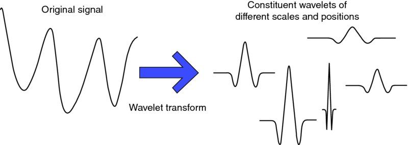
Figure 1.4 Wavelet decomposition.
Two versions of the WT can be distinguished: the continuous wavelet transform (CWT) and the discrete wavelet transform (DWT). The difference between them lies in the set of scales and positions at which each transform operates. The CWT can operate at every scale. However, an upper bound is determined since CWT is extremely computationally expensive. Also, in CWT the analyzing wavelet is shifted smoothly over the full domain of the function analyzed. To reduce the computational burden, wavelet coefficients are calculated only on a subset of scales. This method is called the DWT.
In general, wavelets can be separated in orthogonal and nonorthogonal wavelets. The term wavelet function is used generically to refer to either orthogonal or nonorthogonal wavelets. An orthogonal set of wavelets is called a wavelet basis, and a set of nonorthogonal wavelets is termed a wavelet frame. The use of an orthogonal basis implies the use of the DWT, whereas frames can be used with either the discrete or the continuous transform.
Over the years a substantial number of wavelet functions have been proposed in the literature. The Gaussian, the Morlet, and the Mexican hat wavelets are crude wavelets that can be used only in continuous decomposition. The wavelets in the Meyer wavelet family are infinitely regular wavelets that can be used in both CWT and DWT. The wavelets in the Daubechies, symlet, and coiflet families are orthogonal and compactly supported wavelets. These wavelet families can also be used in CWT and DWT. The B-splines and biorthogonal wavelet families are biorthogonal, compactly supported wavelet pairs that can also be used in both CWT and DWT. Finally, the complex Gaussian, complex Morlet, complex Shannon, and complex-frequency B-spline wavelet families are complex wavelets that can be used in the complex CWT.
Generally, the DWT is used for data compression if the signal is already sampled, and the CWT is used for signal analysis. In the next sections the CWT and the DWT are examined in detail. In Figure 1.5 the Mexican hat wavelet is presented, and in Figures 1.6 and 1.7 two wavelets of the Daubechies family are presented, the Daubechies 3 and 12, respectively. In addition, in Figures 1.6 and 1.7, the scaling functions and decomposition and reconstruction filters are presented with low- and high-pass filters.
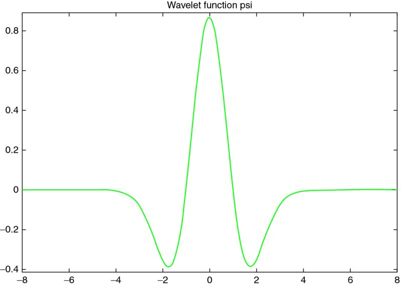
Figure 1.5 Mexican hat wavelet.
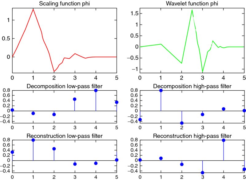
Figure 1.6 Daubechies 3 wavelet (top right) and the scaling function (top left). The decomposition (middle) and reconstruction (bottom) filters are also presented with low-pass (left) and high-pass (right) filters.
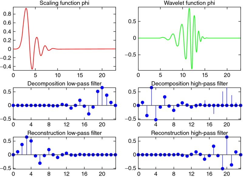
Figure 1.7 The Daubechies 12 wavelet (top right) together with the scaling function (top left). The decomposition (middle) and reconstruction (bottom) filters are also presented with low-pass (left) and high-pass (right) filters.
Continuous Wavelet Transform
Representing a signal as a function f(t), the CWT of this function comprises the wavelet coefficients, C(a, b), which are produced through the convolution of a mother wavelet function, ψ(t), with the signal analyzed, f(t). The CWT is defined as the summation over all time of the signal multiplied by scaled, shifted versions of the wavelet function:
where
The CWT is continuous in the set of scales and positions at which it operates. It is also continuous in terms of shifting; during computation, the analyzing wavelet is shifted smoothly over the full domain of the function analyzed.
Either real or complex analytical wavelets can be used. Complex analytical wavelets can separate amplitude and phase components, while real wavelets are often used to detect sharp signal transitions. The results of the CWT are many wavelet coefficients C, which are a function of scale and position. Multiplying each coefficient by the appropriately scaled and shifted wavelet yields the constituent wavelets of the original signal. As the original signal can be represented in terms of a wavelet expansion (using coefficients in a linear combination of the wavelet functions), data operations can be performed using just the corresponding wavelet coefficients.
Similar to the STFT, the magnitude of wavelet coefficients will be represented by a plot on which the x-axis represents the position along time and the y-axis represents the scale. This plot, called a scalogram, represents the energy density of the signal:
A scalogram allows the changing spectral composition of nonstationary signals to be measured and compared. If the wavelet ![]() and satisfies the admissibility condition
and satisfies the admissibility condition
the original signal can be synthesized from the WT (Daubechies, 1992). The continuous reconstruction formula is given by
Discrete Wavelet Transform
Calculating wavelet coefficients at every possible scale is computationally expensive. However, if we choose only a subset of scales and translations based on powers of 2 (the dyadic lattice), our analysis will be much more efficient and just as accurate (Misiti et al., 2009). We obtain such an analysis from the DWT. In the DWT the wavelet family is taken from a double-indexed regular lattice:
where the parameters p and q denote the step sizes of the dilation and the translation parameters. For p = 2 and q = 1 we have the standard dyadic lattice:
Thus, the scaling function φ generates for each j ∈ Z the sets ![]() , where
, where ![]() denotes the set of integers and
denotes the set of integers and
The basis wavelet functions are usually of the form
It follows that there is a sequence {hk} (where hk is a scaling filter associated with the wavelet) such that ∑|hk|2 = 1 and
where φ is normalized so that ∫∞− ∞φ(t) dt = 1.
When {hk} is finite, a compactly supported scaling function is the solution to the dilation equation above. The wavelet function is defined in terms of the scaling function as
where ∫∞− ∞ψ(t) dt = 0 and gk = ( − 1)k + 1h1 − k is a wavelet filter. Then ![]() is the orthogonal complement of Vj in Vj+1,
is the orthogonal complement of Vj in Vj+1, ![]() .
.
The DWT of the signal function comprises the wavelet coefficients C(j, k), which are produced through the convulsion of a mother wavelet function ψj, k(t)with the signal analyzed, f(t):
Thus, the discrete synthesis of the original signal is
Usually, the low-frequency content is the most important part of a signal. It is what gives the signal its identity, while the high-frequency component usually contains a large part of the noise in the signal (Misiti et al., 2009). We term the high-scale, low-frequency components approximations and the low-scale, high-frequency components details. At each level j, we build the j-level approximation aj, or approximation at level j, and a deviation signal called the j-level detail dj, or detail at level j. The original signal is considered to be the approximation at level zero, denoted a0. The words approximation and detail are justified by the fact that a1 is an approximation of a0 taking into account the low frequencies of a0, whereas the detail d1 corresponds to the high-frequency correction. For additional and detailed expositions on the mathematical aspects of wavelets, we refer, for example, to Daubechies (1992), Kaiser (1994), Kobayashi (1998), Mallat (1999), and Wojtaszczyk (1997).
Neural Networks
Next we present a brief introduction to neural networks. The advantages of neural networks are discussed as well as their applications in finance. In Chapter 2 the mathematical and theoretical aspects are presented analytically.
Artificial neural networks or, simply, neural networks draw their inspiration from biological systems. They are essentially devices of parallel and distributed processing for nonparametric statistical inference which simulate the basic operating principles of the biological brain. They consist of many interconnected neurones (also known as hidden units), whose associated weights determine the strength of the signal passed through them. No particular structure or parametric form is assumed a priori; rather, the strengths of the connections are computed in a way that captures the essential features in the data.
The iterative algorithms employed for this purpose are known as learning algorithms because of their gradual nature. Certain algorithms were firmly positioned in the statistical framework by White (1989) and later by Geman et al. (1992), who demonstrated that they could be formulated as a nonlinear regression problem.
Neural networks are analogous to nonparametric nonlinear regression models, which constitute a very powerful approach, especially for financial applications. More generally, they are essentially statistical tools for performing inductive inference, providing an elegant formalism for unifying different nonparametric paradigms, such as nearest neighbors, kernel smoothers, and projection pursuit. Neural networks have shown considerable successes in a variety of disciplines, ranging through engineering, control, and financial modeling (Zapranis and Refenes, 1999).
In the past 20 years, neural networks have enjoyed a rapid expansion and increasing popularity in both the academic and industrial research communities. Lately, an increased number of studies have been published in various research areas. The main power of neural networks accrues from their capability for universal function approximation. Many studies (e.g., Cardaliaguet and Euvrard, 1992; Cybenko, 1989; Funahashi, 1989; Hornik et al., 1989, 1990; Ito, 1993; White, 1990); have shown that one-hidden-layer neural networks can approximate arbitrarily well any continuous function, including the function's derivatives.
The novelty about neural networks lies in their ability to model nonlinear processes with few (if any) a priori assumptions about the nature of the generating process (Rumelhart et al., 1986). This is particularly useful in investment management, where much is assumed and little is known about the nature of the process determining asset prices.
Modern investment management models, such as the arbitrage pricing theory, rely on the assumption that asset returns can be explained in terms of a set of factors. The usual assumption is that the return of an asset is a linear combination of the asset's exposure to these factors. Such theories have been very useful in expanding our understanding of capital markets, but many financial anomalies have remained unexplainable. In Zapranis and Refenes (1999) the problem of investment management was divided into three parts—factor analysis, estimating returns, and portfolio optimization—and it was shown that neural learning can play a part in each.
Moreover, neural networks are less sensitive than classical approaches to assumptions regarding the error term, and hence they can be used in the presence of noise, chaotic sections, and probability distributions with fat tails. The usual assumptions among financial economists are that price fluctuations not due to external influences are dominated by noise and can be modeled by stochastic processes. As a result, analysts try to understand the nature of noise and develop tools for predicting its effects on asset prices. However, very often, these remaining price fluctuations are due to nonlinear dynamics of the generating process. Therefore, given appropriate tools, it is possible to represent (and possibly understand) more of the market's price structure on the basis of completely or partially deterministic but nonlinear dynamics (Zapranis and Refenes, 1999).
Because of their inductive nature, neural networks have the ability to infer complex nonlinear relationships between an asset price and its determinants. Although, potentially, this approach can lead to better nonparametric estimators, neural networks are not always easily accepted in the financial economics community, mainly because established procedures for testing the statistical significance of the various aspects of the estimated model do not exist. A coherent set of methodologies for developing and assessing neural models, with a strong emphasis on their practical use in the capital markets, was provided by Zapranis and Refenes (1999).
Recently, academic researchers and market participants, have shown an increasing interest in nonlinear modeling techniques, with neural networks assuming a prominent role. Neural networks are being applied to a number of “live” systems in financial engineering and have shown promising results. Various performance figures are being quoted to support these claims, but the absence of explicit models, due to the nonparametric nature of the approach, makes it difficult to assess the significance of the model estimated and the possibility that any short-term success is due to data mining (Zapranis and Refenes, 1999).
Due to their nonparametric nature, neural models are of particular interest in finance, since the deterministic part (if any) of asset price fluctuations is largely unknown and arguably nonlinear. Over the years they have been applied extensively to all stages of investment management. Comprehensive reviews have been provided by Trippi and Turban (1992), and by Vellido et al. (1999).
Among the numerous contributions, notable are applications in bonds by Moody and Utans (1994) and Dutta and Shekhar (1988); in stocks by White (1988), Refenes et al. (1994), and Schöneburg (1990); in foreign exchange by Weigend et al. (1991); in corporate and macroeconomics by Sen et al. (1992); and in credit risk by Atiya (2001).
From a statistical viewpoint, neural networks have a simple interpretation: Given a sample Dn = {(xi; yi)}ni = 1 generated by an unknown function ϕ(x) with the addition of a stochastic zero-mean component ϵ,
the task of “neural learning” is to construct an estimator ![]() of ϕ(x), where w is a set of free parameters known as connection weights. Since no a priori assumptions are made regarding the functional form of ϕ(x), the neural network g(x; w) is a nonparametric estimator of the conditional density E[y|x], as opposed to a parametric estimator, where a priori assumptions are made.
of ϕ(x), where w is a set of free parameters known as connection weights. Since no a priori assumptions are made regarding the functional form of ϕ(x), the neural network g(x; w) is a nonparametric estimator of the conditional density E[y|x], as opposed to a parametric estimator, where a priori assumptions are made.
Nevertheless, knowledge of the relative theory of neural learning and the basic models of neural networks is essential for their effective implementation, especially in complex applications such as the ones encountered in finance. In Chapter 2 an in-depth analysis of neural networks is presented.
Wavelet Neural Networks
Wavelet networks are a new class of networks that combine classic sigmoid neural networks and wavelet analysis. Wavelet networks have been used with great success in a wide range of applications. Wavelet analysis has proved to be a valuable tool for analyzing a wide range of time series and has already been used with success in image processing, signal denoising, density estimation, signal and image compression, and time-scale decomposition. Wavelet analysis is often regarded as a “microscope” in mathematics (Cao et al., 1995), and it is a powerful tool for representing nonlinearities (Fang and Chow, 2006). The major drawback of wavelet analysis is that it is limited to applications of small input dimension. The reason for this is that the construction of a wavelet basis is computationally expensive when the dimensionality of the input vector is relatively high (Zhang, 1997).
On the other hand, neural networks have the ability to approximate any deterministic nonlinear process, with little knowledge and no assumptions regarding the nature of the process. However, classical sigmoid neural networks have a series of drawbacks. Typically, the initial values of the neural network's weights are chosen randomly. Random weight initialization is generally accompanied by extended training times. In addition, when the transfer function is sigmoidal, there is always a significant change: that the training algorithm will converge to local minima. Finally, there is no theoretical link between the specific parameterization of a sigmoidal activation function and the optimal network architecture, that is, model complexity (the opposite holds true for wavelet networks).
Pati and Krishnaprasad (1993) have demonstrated that it is possible to construct a theoretical formulation of a feedforward neural network in terms of wavelet decompositions. WNs were proposed by Zhang and Benveniste (1992) as an alternative to feedforward neural networks which would alleviate the aforementioned weaknesses associated with each method. The wavelet networks are a generalization of radial basis function networks. Wavelet networks are one hidden layer networks that use a wavelet as an activation function instead of the classic sigmoidal family. It is important here to mention that multidimensional wavelets preserve the “universal approximation” property that characterizes neural networks. The nodes (or wavelons) of wavelet networks are wavelet coefficients of the function expansion that have a significant value. Various reasons were presented by Bernard et al. (1998) explaining why wavelets should be used instead of other transfer functions. In particular, first, wavelets have strong compression abilities, and second, computing the value at a single point or updating the function estimate from a new local measure involves only a small subset of coefficients.
Wavelet networks have been used in a variety of applications so far: in short-term load forecasting (Bashir and El-Hawary, 2000; Benaouda et al., 2006; Gao and Tsoukalas, 2001; Ulugammai et al., 2007; Yao et al., 2000); in time-series prediction (Cao et al., 1995; Chen et al., 2006; Cristea et al., 2000); in signal classification and compression (Kadambe and Srinivasan, 2006; Pittner et al., 1998; Subasi et al., 2005); in signal denoising (Zhang, 2007); in statics, and dynamics (Allingham et al., 1998; Oussar and Dreyfus, 2000; Oussar et al., 1998; Pati and Krishnaprasad, 1993; Postalcioglu and Becerikli, 2007; Zhang and Benveniste, 1992); in nonlinear modeling (Billings and Wei, 2005); and in nonlinear static function approximation (Jiao et al., 2001; Szu et al., 1992; Wong and Leung, 1998). Khayamian et al. (2005) even proposed the use of wavelet networks as a multivariate calibration method for simultaneous determination of test samples of copper, iron, and aluminum. Finally, Alexandridis and Zapranis (2013a,b) used wavelet networks in modeling and pricing financial weather derivatives.
In contrast to classical sigmoid neural networks, wavelet networks allow for constructive procedures that efficiently initialize the parameters of a network. Using wavelet decomposition a wavelet library can be constructed. In turn, each wavelon can be constructed using the best wavelet in the wavelet library. As a result, wavelet networks provide information for the relative participation of each wavelon to the function approximation and the estimated dynamics of the generating process. The main characteristics of these constructive procedures are (1) convergence to the global minimum of the cost function, and (2) the initial weight vector being in close proximity to the global minimum, resulting in drastically reduced training times (Zhang, 1997; Zhang and Benveniste, 1992). Finally, efficient initialization methods will approximate the same vector of weights, minimizing the loss function each time.
Applications of Wavelet Neural Networks in Financial Engineering, Chaos, and Classification
Artificial intelligence and machine learning are used to improve the process of decision making in a wide range of financial applications. For example, they are used to evaluate credit risk, for risk assessment of mortgage loans, in project management and bidding strategies, in financial and economic forecasting, in risk assessment of investments in fixed-income products traded on an exchange, to identify regularities in price changes of securities, and to predict default risk. Other applications explored recently are portfolio selection and diversification, simulation of market behavior, and pattern identification in financial data.
During recent years, neural networks have been utilized extensively in various fields in finance. For example, Moody and Utans (1994) employed neural network in corporate bond rating prediction. Neural networks were used in securities trading by Trippi and Turban (1992) and Zapranis and Refenes (1999), and Chen et al. (2003) used them to forecast and trade the Taiwan stock index. Finally, neural networks were utilized for bankruptcy prediction by Tam and Kiang (1992) and Wilson and Sharda (1994).
On the other hand, wavelet networks have been introduced only recently in financial applications. As a result, the literature on the application of wavelet network in finance is limited. As an intermediate step, a very popular technique is to apply wavelet analysis to decompose a financial time series and then use the decomposed part or the wavelet coefficients as inputs to a neural network.
Becerra et al. (2005) used wavelet networks for the identification and prediction of corporate financial distress. More precisely, the authors used various financial ratios, such as working capital/total assets, accumulated retained profit/total assets, profit before interest, and tax/total assets. They collected data between 1997 and 2000 from 60 British firms and compared three models. The first one was a linear model; the other two were nonlinear nonparametric neural networks and wavelet networks. Their results indicate that the wavelet networks outperform the other two alternatives in classifying corporate financial distress correctly.
In a similar application wavelet networks were trained in predicting bankruptcy (Chauhan et al., 2009). Three data sets were used to test their model. The wavelet network was evaluated as to bankruptcy prediction for 129 U.S. banks, 66 Spanish banks, and 40 Turkish banks. Their results show high accuracy and conclude that wavelet networks are a very effective tool for classification problems.
Echauz and Vachtsevanos (1997) used wavelet networks as trading advisors. Based on past data, the investor had to decide whether to switch in or out of an S&P index fund. The decisions suggested by the wavelet networks were based on a 13-week holding period yield. Their results indicated that wavelet networks exceeded the performance of a simple buy-and-hold strategy.
Wavelet analysis was used by Aussem et al. (1998) to decompose the S&P index. The daily price index was decomposed on various scales, and then the coefficients of the wavelet decompositions were used as the input to a network to forecast the future price of the index up to five days ahead.
Similarly, wavelet analysis and radial basis function neural networks (a subclass of wavelet networks) were combined by Liu et al. (2004). The two methods were combined to identify and analyze possible chart patterns, and a method of financial forecasting using technical analysis was presented. Their results indicate that the matching method proposed can be used to automate the chart pattern-matching process.
Bashir and El-Hawary (2000) applied a wavelet network to short-term load forecasting. Similarly, Benaouda et al. (2006), Gao and Tsoukalas (2001), and Ulugammai et al. (2007) utilized different versions of wavelet networks and wavelet analysis for accurate forecasting of electricity loads, a necessity in the management of energy companies. Pindoriya et al. (2008) utilized wavelet networks in energy price forecasting in electricity markets.
Wavelet networks have also been used to analyze financial time series (Alexandridis and Zapranis, 2013a,b; Zapranis and Alexandridis, 2011). More precisely, wavelet networks were employed in the context of weather derivative pricing and modeling. Moreover, trained wavelet networks were used to predict the future prices of financial weather derivatives. Their findings suggest that wavelet networks can model the underlying processes very well and thus constitute a very accurate and efficient tool for weather derivative pricing.
Wavelet networks were applied to the oil market by Alexandridis et al. (2008). The objective was to investigate the factors that affect crude oil price for the period 1988 to 2008 through comparison of a linear and a nonlinear approach. The dynamics of the West Texas Intermediate crude oil price, time series as well as the relation of crude oil price, and returns to various explanatory variables were studied. First, wavelet analysis was used to extract the driving forces and dynamics of crude oil price and returns processes. Also examined was whether a wavelet neural network estimator could provide some incremental value toward understanding the crude oil price process. In contrast to the linear model, it was determined that wavelet network findings are in line with those of economic analysts. Wavelet networks not only have better predictive power in forecasting crude oil returns but can also model the dynamics of the returns correctly.
Alexandridis and Hasan (2013) investigated the impact of the global financial crisis on the multihorizon nature of systematic risk and market risk using daily data from eight major European equity markets over the period 2005 to 2012. The method was based on a wavelet multiscale approach within the framework of a capital asset pricing model. The sample covers pre-crisis, crisis, and post-crisis periods with varying experiences and regimes. The results indicate that beta coefficients have a mutliscale tendency in sample countries. Moreover, wavelet networks were trained using past data to forecast the post-crisis multiscale betas and the value at risk in each market.
In addition, wavelet networks have been employed extensively in classification problems in various disciplines other than finance: for example, in medicine in recognition of cardiac arythmias (Lin et al., 2008) and breast cancer (Senapati et al., 2011) and for EEG signal classification (Subasi et al., 2005); by Szu et al. (1992) for signal classification and by Shi et al. (2006) for speech signal processing. Finally, wavelet networks were utilized successfully for the prediction of chaotic time series (Cao et al., 1995; Chen et al., 2006; Cristea et al., 2000).
Building Wavelet Networks
In this book we focus on the construction of optimal wavelet networks and their successful application in a wide range of applications. A generally accepted framework for applying wavelet networks is missing from the literature. In this book we present a complete statistical model identification framework in order to employ wavelet networks in various applications. To our knowledge, we are the first to do so. Although a vast literature on wavelet networks exists, to our knowledge this is the first study that presents a step-by-step guide for model identification for wavelet networks. Model identification can be classified in two parts: model selection and variable significance testing. In this study, a framework similar to the one proposed by Zapranis and Refenes (1999) for classical sigmoid neural networks is adapted. More precisely, the following subjects were examined thoroughly: the structure of a wavelet network, training methods, initialization algorithms, variable significance and variable selection algorithms, model selection methods, and methods to construct confidence and prediction intervals. Some of these issues were studied to some extent by Iyengar et al. (2002).
Moreover, to succeed in the use of wavelet networks, a model adequacy framework is needed. The evaluation of the model is usually performed in two stages. In the first the accuracy of the predictions is assessed and in the second the performance and behavior of the wavelet network are evaluated under conditions as close as possible to the actual operating conditions of the application.
Variable Selection
In the following chapters, the first part of model identification, variable selection, is discussed analytically. The objective is to develop an algorithm to use to select the statistically significant variables from a group of candidates in a problem where little theory is available. Our aim is to present a statistical procedure that produces robust and stable results when it is applied in the wavelet network framework.
In real problems it is important to determine the independent variables correctly, for various reasons. In most financial problems there is little theoretical guidance and information about the relationship of any explanatory variable with the dependent variable. Irrelevant variables are among the most common sources of specification error. An unnecessary independent variable included in a model (e.g., in the training of a wavelet network) creates a series of problems. First, the architecture of the wavelet network increases. As a result, the training time of the wavelet network and the computational burden can increase significantly. Moreover, there is a possibility that the inclusion of irrelevant variables will affect the training of the wavelet network. As presented for complex problems in subsequent chapters, when irrelevant variables are included there is a possibility that the training algorithm will be trapped in a local minimum during minimization of the loss function. Finally, when irrelevant variables are included in the model, its predictive power and generalization ability are reduced.
On the other hand, correctly specified models are easier to understand and interpret. The underlying relationship is explained by only a few key variables, while all minor and random influences are attributed to the error term. Finally, including a large number of independent variables relative to sample size runs the risk of a spurious fit.
To select the statistically significant and relevant variable, from a group of possible explanatory variables, hypotheses tests of statistical significance are used. To do so, the relative contributions of the explanatory variables in explaining the dependent variable in the context of a specific model are estimated. Then the significance of a variable is assessed. This can be done by testing the null hypothesis that it is irrelevant, either by comparing a test statistic that has a known theoretical distribution with its critical value, or by constructing confidence intervals for the relevance criterion. Our decision on rejecting or not rejecting the null hypothesis is based on a given significance level. The p-value, the smallest significance level for which the null hypothesis will not be refuted, imposes a ranking on the variables according to their relevance to the particular model (Zapranis and Refenes, 1999).
Before proceeding to variable selection, a measure of relevance must be defined. Various measures are tested in later chapters, and an algorithm that produces robust and stable results is presented.
Model Selection
Next, the second part of model identification, variable selection, will be discussed analytically. The objective is to find a statistical procedure that identifies correctly the optimal number of wavelons (hidden units) that are needed to model a specific problem. One of the most crucial steps is to identify the correct topology of the network. A desired wavelet network architecture should contain as few hidden units as necessary while explaining as much variability of the training data as possible. A network with fewer hidden units than needed would not be able to learn the underlying function, while selecting more hidden units than needed will result in an overfitted model.
In both cases, the results obtained from the wavelet network cannot be interpreted. Moreover, an underfitted or overfitted network cannot be used to forecast the evolution of the underlying process. In the first case the model has not learned the dynamics of the underlying process, hence cannot be used for forecasting. On the other hand, in an overfitted network, the model has learned the noise part; hence, any forecasts will be affected by the noise and will differ significantly from the real target values. Therefore, an algorithm to select the appropriate wavelet network model for a given problem must be derived.
Model Adequacy Testing
After the construction of a wavelet network, we are interested in measuring its predictive ability in the context of a particular application. The evaluation of the model usually includes two clearly distinct, though related stages. In the first stage, various metrics that quantify the accuracy of the predictions or the classifications made by the model are used and the model is evaluated based on these metrics. The term accuracy is a quantification of the “proximity” between the outputs of the wavelet network and the target values desired. Measurements of the precision are related to the error function that is minimized (or in some cases, the profit function that is maximized) during the model specification of the wavelet network model.
The second step is to assess the behavior and performance of the wavelet network model under conditions as close as possible to the actual operating conditions of the application. The greater accuracy of the network model does not necessarily mean that it will be applied successfully. It is important, therefore, that the performance of the model be evaluated in the context of the decision-making system that it supports. Especially for use in time-series forecasting application, the performance and evaluation of the model should be based on benchmark trading strategies. It is also important to evaluate the behavior of the model throughout the range of the actual scenarios possible. For example, if the application concerns the prediction of the performance of a stock index, it would not be correct if the validation sample corresponds solely to a period with a strong upward trend, since the evaluation will be restricted to the specific circumstances.
A full understanding of the behavior of the model under a variety of conditions is a prerequisite for the creation of a successful decision support system or simply a decision-making system (e.g., automated trading systems). In upcoming chapters, an analytical model adequacy framework is presented.
Book Outline
The purpose of the book is twofold: first, to expand the framework that was developed by Alexandridis (2010) for model selection and variable selection in the framework of wavelet networks; and second, to provide a textbook that presents a step-by-step guide to employing wavelet networks in various applications (finance, classification, chaos, etc.).
Chapter 2: Neural Networks
In this chapter the basic aspects of the neural networks are presented: more precisely, the delta rule, the backpropagation algorithm, and the concept of training a network. Our purpose is to make the reader familiar with the basic concepts of the neural network framework. These concepts are later modified to construct a new class of neural networks called wavelet networks.
Chapter 3: Wavelet Neural Networks
The basic aspects of the wavelet networks are presented in this chapter: more precisely, the structure of a wavelet network, various initialization methods, a training method for the wavelet networks, and stopping conditions of the training. In addition, online training is discussed and various initialization methods are compared and evaluated in two case studies.
Chapter 4: Model Selection: Selecting the Architecture of the Network
Chapter 4 we describe the model selection procedure. One of the most crucial steps is to identify the correct topology of the network. Various algorithms and criteria are presented as well as a complete statistical framework. Finally, the various methods are compared and evaluated in two case studies.
Chapter 5: Variable Selection: Determining the Explanatory Variables
In this chapter various methods of testing the significance of each explanatory variable are presented and tested. The purpose of this section is to find an algorithm that gives consistently stable and correct results when it is used with wavelet networks. In real problems it is important to determine correctly the independent variables. In most problems there is only limited information about the relationship of any explanatory variable with the dependent variable. As a result, unnecessary independent variables are included in the model, reducing its predictive power. Finally, the various methods are compared and evaluated in two case studies.
Chapter 6: Model Adequacy Testing: Determining a Network's Future Performance
In this chapter we present various methods used to test the adequacy of the wavelet network constructed. Various criteria are presented that examine the residuals of the wavelet network. Moreover, depending on the application (classification or prediction), additional evaluation criteria are presented and discussed.
Chapter 7: Modeling Uncertainty: From Point Estimates to Prediction Intervals
The framework proposed is expanded by presenting two methods of estimating confidence and prediction intervals. The output of the wavelet networks is the approximation of the underlying function obtained from noisy data. In many applications, especially in finance, risk managers may be more interested in predicting intervals for future movements of the underlying function than in simply point estimates. In addition, the methods proposed are compared and evaluated in two case studies.
Chapter 8: Modeling Financial Temperature Derivatives
In this chapter a real data set is used to demonstrate the application of our proposed framework to a financial problem. More precisely, using data from detrended and deseasonalized daily average temperatures, a wavelet network is constructed, initialized, and trained, in the context of modeling and pricing financial weather derivatives. At the same time the significant variables are selected: in this case, the correct number of lags. Finally, the wavelet network developed will be used to construct confidence and prediction intervals.
Chapter 9: Modeling Financial Wind Derivatives
In this chapter, the framework proposed is applied to a second financial data set. More precisely, daily average wind speeds are modeled and forecast in the context of modeling and pricing financial weather derivatives. At the same time, the significant variables are selected: in this case, the correct number of lags. Finally, the wavelet network developed will be used to forecast the future index of the wind derivatives.
Chapter 10: Predicting Chaotic Time Series
In this chapter the framework proposed is evaluated for modeling and predicting chaotic time series. More precisely, the chaotic system is described by the Mackey–Glass equation. A wavelet network is constructed and then used to predict the evolution of the chaotic system and construct confidence and prediction intervals.
Chapter 11: Classification of Breast Cancer Cases
In this chapter the framework proposed in the earlier chapters is applied in a real-life application. In this case study a wavelet network is constructed to classify breast cancer based on various attributes. Each instance has one of two possible classes: benign or malignant. The aim is to construct a wavelet network that accurately classifies each clinical case. The classification is based on nine attributes: clump thickness, uniformity of cell size, uniformity of cell shape, marginal adhesion, single epithelial cell size, bare nuclei, bland chromatin, normal nucleoli, and mitoses.
References
- Alexandridis, A. (2010). “Modelling and pricing temperature derivatives using wavelet networks and wavelet analysis,” University of Macedonia, Thessaloniki, Greece.
- Alexandridis, A., and Hasan, M. (2013). “Global financial crisis and multiscale systematic risk: evidence from selected european markets.” In The Impact of the Global Financial Crisis: on Banks, Financial Markets and Institutions in Europe, University of Southampton, UK.
- Alexandridis, A., and Livanis, S. (2008). “Forecasting crude oil prices using wavelet neural networks.” 5th ΦΣΔΕΤ Athens, Greece.
- Alexandridis, A., and Zapranis, A. (2013a). “Wind derivatives: modeling and pricing.” Computational Economics, 41(3), 299–326.
- Alexandridis, A. K., and Zapranis, A. D. (2013b). Weather Derivatives: Modeling and Pricing Weather-Related Risk. Springer-Verlag, New York.
- Alexandridis, A., Zapranis, A., and Livanis, S. (2008). “Analyzing crude oil prices and returns using wavelet analysis and wavelet networks.” 7th HFAA, Chania, Greece.
- Allen, J. B. (1982). “Application of the short-time Fourier transform to speech processing and spectral analysis.” IEEE ICASSP, 1012–1015.
- Allingham, D., West, M., and Mees, A. I. (1998). “Wavelet reconstruction of nonlinear dynamics.” International Journal of Bifurcation and Chaos, 8(11), 2191–2201.
- Atiya, A. F. (2001). “Bankruptcy prediction for credit risk using neural networks: A survey and new results.” IEEE Transactions on Neural Networks, 12(4), 929–935.
- Aussem, A., Campbell, J., and Murtagh, F. (1998). “Wavelet-based feature extraction and decomposition strategies for financial forecasting.” Journal of Computational Intelligence in Finance, 6, 5–12.
- Bashir, Z., and El-Hawary, M. E. (2000). “Short term load forecasting by using wavelet neural networks.” Proceedings of Canadian Conference on Electrical and Computer Engineering, 163–166.
- Becerra, V. M., Galvão, R. K., and Abou-Seada, M. (2005). “Neural and wavelet network models for financial distress classification.” Data Mining and Knowledge Discovery, 11(1), 35–55.
- Benaouda, D., Murtagh, G., Starck, J.-L., and Renaud, O. (2006). “Wavelet-based nonlinear multiscale decomposition model for electricity load forecasting.” Neurocomputing, 70, 139–154.
- Bernard, C., Mallat, S., and Slotine, J.-J. (1998). “Wavelet interpolation networks.” Proceedings of ESANN ‘98, Bruges, Belgium, 47–52.
- Billings, S. A., and Wei, H.-L. (2005). “A new class of wavelet networks for nonlinear system identification.” IEEE Transactions on Neural Networks, 16(4), 862–874.
- Black, F., and Scholes, M. (1973). “The pricing of options and corporate liabilities.” Journal of Political Economy, 81(3), 637–654.
- Bracewell, R. N. (2000). The Fourier Transform and Its Applications. McGraw-Hill, New York.
- Cao, L., Hong, Y., Fang, H., and He, G. (1995). “Predicting chaotic time series with wavelet networks.” Physica, D85, 225–238.
- Cardaliaguet, P., and Euvrard, G. (1992). “Approximation of a function and its derivative with a neural network.” Neural Networks, 5(2), 207–220.
- Chauhan, N., Ravi, V., and Karthik Chandra, D. (2009). “Differential evolution trained wavelet neural networks: application to bankruptcy prediction in banks.” Expert Systems with Applications, 36(4), 7659–7665.
- Chen, A.-S., Leung, M. T., and Daouk, H. (2003). “Application of neural networks to an emerging financial market: forecasting and trading the Taiwan stock index.” Computers and Operations Research, 30(6), 901–923.
- Chen, Y., Yang, B., and Dong, J. (2006). “Time-series prediction using a local linear wavelet neural wavelet.” Neurocomputing, 69, 449–465.
- Cristea, P., Tuduce, R., and Cristea, A. (2000). “Time series prediction with wavelet neural networks.” Proceedings of 5th Seminar on Neural Network Applications in Electrical Engineering, Belgrade, Yugoslavia, 5–10.
- Cybenko, G. (1989). “Approximation by superpositions of a sigmoidal function.” Mathematics of Control, Signals and Systems, 2(4), 303–314.
- Daubechies, I. (1992). Ten Lectures on Wavelets. SIAM, Philadelphia.
- Donoho, D. L., and Johnstone, I. M. (1994). “Ideal spatial adaption by wavelet shrinkage.” Biometrika, 81, 425–455.
- Dutta, S., and Shekhar, S. (1988). “Bond rating: a nonconservative application of neural networks.” IEEE International Conference on Neural Networks, 443–450.
- Echauz, J., and Vachtsevanos, G. (1997). “Separating order from disorder in a stock index using wavelet neural networks.” EUFIT, 97, 8–11.
- Fang, Y., and Chow, T. W. S. (2006). “Wavelets based neural network for function approximation.” Lecture Notes in Computer Science, 3971, 80–85.
- Fernandez, V. P. (2005). “The international CAPM and a wavelet-based decomposition of value at risk.” Studies in Nonlinear Dynamics and Econometrics, 9(4).
- Fernandez, V. (2006). “The CAPM and value at risk at different time-scales.” International Review of Financial Analysis, 15(3), 203–219.
- Finnerty, J. D. (1988). “Financial engineering in corporate finance: an overview.” Financial Management, 14–33.
- Funahashi, K.-I. (1989). “On the approximate realization of continuous mappings by neural Networks.” Neural networks, 2(3), 183–192.
- Gao, R., and Tsoukalas, H. I. (2001). “Neural-wavelet methodology for load forecasting.” Journal of Intelligent and Robotic Systems, 31, 149–157.
- Geman, S., Bienenstock, E., and Doursat, R. (1992). “Neural networks and the bias/variance dilemma.” Neural Computation, 4(1), 1–58.
- Gençay, R., Selçuk, F., and Whitcher, B. (2003). “Systematic risk and timescales.” Quantitative Finance, 3, 108–116.
- Gençay, R., Selçuk, F., and Whitcher, B. (2005). “Multiscale systematic risk.” Journal of International Money and Finance, 24(1), 55–70.
- Grossmann, A., and Morlet, J. (1984). “Decomposition of Hardy functions intro square-integrable wavelets of constant shape.” SIAM Journal of Mathematical Analysis, 15(4), 723–736.
- Hawley, D. D., Johnson, J. D., and Raina, D. (1990). “Artificial neural systems: a new tool for financial decision-making.” Financial Analysts Journal, 63–72.
- He, K., Lai, K. K., and Yen, J. (2012). “Ensemble forecasting of value at risk via multi resolution analysis based methodology in metals markets.” Expert Systems with Applications, 39(4), 4258–4267.
- Hornik, K., Stinchcombe, M., and White, H. (1989). “Multilayer feedforward networks are universal approximators.” Neural Networks, 2(5), 359–366.
- Hornik, K., Stinchcombe, M., and White, H. (1990). “Universal approximation of an unknown mapping and its derivatives using multilayer feedforward networks.” Neural Networks, 3(5), 551–560.
- Huang, C.-f., and Litzenberger, R. H. (1988). Foundations for Financial Economics. North-Holland, New York.
- In, F., and Kim, S. (2006a). “The hedge ratio and the empirical relationship between the stock and futures markets: a new approach using wavelet analysis.” Journal of Business, 79(2), 799–820.
- In, F., and Kim, S. (2006b). “Multiscale hedge ratio between the Australian stock and futures markets: Evidence from wavelet analysis.” Journal of Multinational Financial Management, 16(4), 411–423.
- In, F., and Kim, S. (2007). “A note on the relationship between Fama–French risk factors and innovations of ICAPM state variables.” Finance Research Letters, 4(3), 165–171.
- Ito, Y. (1993). “Extension of approximation capability of three layered neural networks to derivatives.” IEEE International Conference on Neural Networks, pp. 377–381.
- Iyengar, S. S., Cho, E. C., and Phoha, V. V. (2002). Foundations of Wavelet Networks and Applications. CRC Press, Grand Rapids, MI.
- Jiao, L., Pan, J., and Fang, Y. (2001). “Multiwavelet neural network and its approximation properties.” IEEE Transactions on Neural Networks, 12(5), 1060–1066.
- Kadambe, S., and Srinivasan, P. (2006). “Adaptive wavelets for signal classification and compression.” International Journal of Electronics and Communications, 60, 45–55.
- Kaiser, G. (1994). A Friendly Guide To Wavelets. Birkhauser, Cambridge, MA.
- Khayamian, T., Ensafi, A. A., Tabaraki, R., and Esteki, M. (2005). “Principal component-wavelet networks as a new multivariate calibration model.” Analytical Letters, 38(9), 1447–1489.
- Kim, S., and In, F. (2005). “The relationship between stock returns and inflation: new evidence from wavelet analysis.” Journal of Empirical Finance, 12, 435–444.
- Kim, S., and In, F. (2007). “On the relationship between changes in stock prices and bond yields in the G7 countries: wavelet analysis.” Journal of International Financial Markets, Money and Finance, 17, 167–179.
- Kobayashi, M. (1998). Wavelets and Their Applications. SIAM, Philadelphia.
- Lim, J. S. (1990). Two-Dimensional Signal And Image Processing. Prentice Hall, Englewood Cliffs, NJ.
- Lin, C.-H., Du, Y.-C., and Chen, T. (2008). “Adaptive wavelet network for multiple cardiac arrhythmias recognition.” Expert Systems with Applications, 34(4), 2601–2611.
- Liu, J. N. K., Kwong, R. W. M., and Bo, F. (2004). “Chart patterns recognition and forecast using wavelet and radial basis function networks.” Lecture Notes in Computer Science, 3214, 564–571.
- Maharaj, E. A., Galagedera, D. U. A., and Dark, J. (2011). “A comparison of developed and emerging equity market return volatility at different time scales.” Managerial Finance, 37(10), 940–952.
- Mallat, S. G. (1999). A Wavelet Tour of Signal Processing. Academic Press, San Diego, CA.
- Marshall, and Bansal, V. K. (1992). Financial Engineering: A Complete Guide to Financial Innovation. New York Institute of Finance, New York.
- Masih, M., Alzahrani, M., and Al-Titi, O. (2010). “Systematic risk and time scales: new evidence from an application of wavelet approach to the emerging Gulf stock markets.” International Review of Financial Analysis, 19(1), 10–18.
- Mason, S. P., Merton, R. C., Perold, A. F., and Tufano, P. (1995). Cases in Financial Engineering: Applied Studies of Financial Innovation, Prentice Hall, Englewood Cliffs, NJ.
- Misiti, M., Misiti, Y., Oppenheim, G., and Poggi, J.-M. (2009). Wavelet Toolbox 4: User's Guide. MathWorks.
- Moody, J. E., and Utans, J. (1994). “Architecture selection strategies for neural networks: Application to corporate bond rating prediction.” In Neural Networks in the Capital Markets, A. P. Refenes, ed. Wiley, New York.
- Mulvey, J. M., Rosenbaum, D. P., and Shetty, B. (1997). “Strategic financial risk management and operations research.” European Journal of Operational Research, 97(1), 1–16.
- Nawab, S., Quatieri, T., and Lim, J. (1983). “Signal reconstruction from short-time Fourier transform magnitude.” IEEE Transactions on Acoustics, Speech, Signal Processing, 31, 986–998.
- Norsworthy, J. R., Li, D., and Gorener, R. (2000). “Wavelet-based analysis of time series: an export from engineering to finance.” Proceedings of the 2000 IEEE, 126–132.
- Oppenheim, A., Schafer, R., and Buck, J. (1999). Discrete Time Signal Processing. Prentice Hall, Englewood Cliffs, NJ.
- Oussar, Y., and Dreyfus, G. (2000). “Initialization by selection for wavelet network training.” Neurocomputing, 34, 131–143.
- Oussar, Y., Rivals, I., Presonnaz, L., and Dreyfus, G. (1998). “Trainning wavelet networks for nonlinear dynamic input output modelling.” Neurocomputing, 20, 173–188.
- Pati, Y. C., and Krishnaprasad, P. S. (1993). “Analysis and synthesis of feedforward neural networks using discrete affine wavelet transforms.” IEEE Transactions on Neural Networks, 4(1), 73–85.
- Pindoriya, N., Singh, S., and Singh, S. (2008). “An adaptive wavelet neural network-based energy price forecasting in electricity markets.” IEEE Transactions on Power Systems, 23(3), 1423–1432.
- Pittner, S., Kamarthi, S. V., and Gao, Q. (1998). “Wavelet networks for sensor signal classification in flank wear assessment.” Journal of Intelligent Manufacturing, 9, 315–322.
- Postalcioglu, S., and Becerikli, Y. (2007). “Wavelet networks for nonlinear system modelling.” Neural Computing and Applications, 16, 434–441.
- Rabeh, K. K., and Mohamed, B. B. (2011). “A time-scale analysis of systematic risk: wavelet-based approach.” Munich Personal RePEc Archive, Paper No. 31938, http://mpra.ub.uni-muenchen.de/31938/
- Ramsey, J. B. (1999). “The contribution of wavelets to the analysis of economic and financial data.” Philosophical Transactions: Mathematical, Physical and Engineering Sciences, 357(1760), 2593–2606.
- Refenes, A., Zapranis, A., and Francis, G. (1994). “Stock performance modeling using neural networks: a comparative study with regression models.” Neural Networks, 7(2), 375–388.
- Rua, A., and Nunes, L. C. (2012). “A wavelet-based assessment of market risk: the emerging markets case.” Quarterly Review of Economics and Finance, 52(1), 84–92.
- Rumelhart, D. E., McClelland, J. L., and University of California–San Diego PDP Research Group. (1986). Parallel Distributed Processing: Explorations in the Microstructure of Cognition. MIT Press, Cambridge, MA.
- Schöneburg, E. (1990). “Stock price prediction using neural networks: a project report.” Neurocomputing, 2(1), 17–27.
- Sen, T., Oliver, R., and Sen, N. (1992). “Predicting Corporate Mergers Using Backpropagation Neural Networks: A Comparative Study with Logistic Models.” Department of Accounting, RB Pamblin College of Business, Virginia Tech, Blacksburg, VA.
- Senapati, M., Mohanty, A., Dash, S., and Dash, P. (2011). “Local linear wavelet neural network for breast cancer recognition.” Neural Computing and Applications, 1–7.
- Shi, D., Chen, F., Ng, G. S., and Gao, J. (2006). “The construction of wavelet network for speech signal processing.” Neural Computing and Applications, 15, 217–222.
- Subasi, A., Alkan, A., Koklukaya, E., and Kiymik, M. K. (2005). “Wavelet neural network classification of EEG signals by using AR model with MLE pre-processing.” Neural Networks, 18, 985–997.
- Szu, H., Telfer, B., and Kadambe, S. (1992). “Neural network adaptive wavelets for signal representation and classification.” Optical Engineering, 31, 1907–1916.
- Tam, K. Y., and Kiang, M. Y. (1992). “Managerial applications of neural networks: the case of bank failure predictions.” Management Science, 38(7), 926–947.
- Trippi, R. R., and Turban, E. (1992). Neural Networks in Finance and Investing: Using Artificial Intelligence to Improve Real World Performance. McGraw-Hill, New York.
- Ulugammai, M., Venkatesh, P., Kannan, P. S., and Padhy, N. P. (2007). “Application of bacterial foraging technique trained artificial and wavelet neural networks in load forecasting.” Neurocomputing, 70, 2659–2667.
- Vellido, A., Lisboa, P. J., and Vaughan, J. (1999). “Neural networks in business: a survey of applications (1992–1998).” Expert Systems with Applications, 17(1), 51–70.
- Walker, J. S. (2008). A Primer on Wavelets and Their Scientific Applications, Chapman and Hall, New York.
- Weigend, A. S., Rumelhart, D. E., and Huberman, B. A. (1991). “Generalization by weight-elimination applied to currency exchange rate prediction.” IJCNN-91-Seattle International Joint Conference on Neural Networks, 837–841.
- White, H. (1988). “Economic prediction using neural networks: the case of IBM daily stock returns.” IEEE International Conference on Neural Networks, 451–458.
- White, H. (1989). “Learning in artificial neural networks: a statistical perspective.” Neural Computation, 1, 425–464.
- White, H. (1990). “Connectionist nonparametric regression: multilayer feedforward networks can learn arbitrary mappings.” Neural Networks, 3(5), 535–549.
- Wilson, R. G. (1995). Fourier Series and Optical Transform Techniques in Contemporary Optics. Wiley, New York.
- Wilson, R. L., and Sharda, R. (1994). “Bankruptcy prediction using neural networks.” Decision Support Systems, 11(5), 545–557.
- Wojtaszczyk, P. (1997). A Mathematical Introduction to Wavelets. Cambridge University Press, Cambridge, UK.
- Wong, K.-W., and Leung, A. C.-S. (1998). “On-line successive synthesis of wavelet networks.” Neural Processing Letters, 7, 91–100.
- Yao, S. J., Song, Y. H., Zhang, L. Z., and Cheng, X. Y. (2000). “Wavelet transform and neural networks for short-term electrical load forecasting.” Energy Conversion and Management, 41, 1975–1988.
- Yousefi, S., Weinreich, I., and Reinarz, D. (2005). “Wavelet-based prediction of oil prices.” Chaos, Solitons and Fractals, 25(2), 265–275.
- Zapranis, A., and Alexandridis, A. (2006). “Wavelet Analysis and Weather Derivatives Pricing.” 5th Hellenic Finance and Accounting Association, Thessaloniki, Greece.
- Zapranis, A., and Alexandridis, A. (2008). “Modelling temperature time dependent speed of mean reversion in the context of weather derivetive pricing.” Applied Mathematical Finance, 15(4), 355–386.
- Zapranis, A., and Alexandridis, A. (2009). “Weather derivatives pricing: modelling the seasonal residuals variance of an ornstein–uhlenbeck temperature process with neural networks.” Neurocomputing, 73, 37–48.
- Zapranis, A., and Alexandridis, A. (2011). “Modeling and forecasting cumulative average temperature and heating degree day indices for weather derivative pricing.” Neural Computing and Applications, 20(6), 787–801.
- Zapranis, A., and Refenes, A. P. (1999). Principles of Neural Model Indentification, Selection and Adequacy: With Applications to Financial Econometrics. Springer-Verlag, New York.
- Zapranis, A., and Sivridis, S. (2003). “Extending Vasicek with neural regression.” Neural Network World, 13(2), 187–210.
- Zhang, Q. (1997). “Using wavelet network in nonparametric estimation.” IEEE Transactions on Neural Networks, 8(2), 227–236.
- Zhang, Q., and Benveniste, A. (1992). “Wavelet networks.” IEEE Transactions on Neural Networks, 3(6), 889–898.
- Zhang, Z. (2007). “Learning algorithm of wavelet network based on sampling theory.” Neurocomputing, 71(1), 224–269.
- Ζαπράνης, Α. (2005). Χρηματοιοκονομική και Νευρωνικά Συστήματα, Κλειδάριθμος, Αθήνα.