
3
Wavelet Neural Networks
In the literature, various versions of wavelet networks have been proposed. A wavelet network usually has the form of a three-layer network. The lower layer represents the input layer, the middle layer is the hidden layer, and the upper layer is the output layer. The way that the three layers are connected and interact defines the structure of the network. In the input layer, the explanatory variables are inserted in the model and transformed to wavelets. The hidden layer consists of wavelons, or hidden units. Finally, all the wavelons are combined to produce the output of the network, ![]() , at the output layer, which is an approximation of the target value, yp.
, at the output layer, which is an approximation of the target value, yp.
In this chapter we present and discuss analytically the structure of the wavelet network proposed. More precisely, in this book, a multidimensional WN with a linear connection between the wavelons and the output is implemented. In addition, there is a direct connection from the input layer to the output layer that will help the network to perform well in linear applications. In other words, a wavelet network with zero hidden units is reduced to a linear model.
Furthermore, the initialization phase, the training phase, and the stopping conditions are discussed. A wavelet is a waveform of effectively limited duration that has an average value of zero and localized properties. Hence, in wavelet networks, selecting initial values of the dilation and translation parameters randomly may not be suitable, since random initialization may lead to wavelons with a value of zero. Four methods for the initialization of the parameters of a wavelet network are presented and evaluated. The simplest is the heuristic method. More sophisticated methods, such as residual-based selection, selection by orthogonalization, and backward elimination, can be used for efficient initialization. The parameters of the wavelet network are further optimized during the training phase. In the training phase the parameters are changed to minimize an error function between the target values and the wavelet output. This is done iteratively until the one of the stopping conditions is met.
Wavelet Neural Networks for Multivariate Process Modeling
Structure of a Wavelet Neural Network
In this section the structure of a wavelet network is presented and discussed. A wavelet network usually has the form of a three-layer network. The lower layer represents the input layer, the middle layer is the hidden layer, and the upper layer is the output layer. In the input layer the explanatory variables are introduced to the wavelet network. The hidden layer consists of hidden units (HUs). The hidden units, also referred to as wavelons, are similar to neurons in the classical sigmoid neural networks. In the hidden layer the input variables are transformed to a dilated and translated version of the mother wavelet. Finally, in the output layer, the approximation of the target values is estimated.
Various structures of a wavelet network have been proposed. The idea of a wavelet network is to adapt the wavelet basis to the training data. Hence, the wavelet estimator is expected to be more efficient than a sigmoid neural network (Zhang, 1993). An adaptive wavelet network was used by Billings and Wei (2005), Kadambe and Srinivasan (2006), Mellit et al. (2006), and Xu and Ho (1999). Chen et al. (2006) proposed a local linear wavelet network. The difference is that the weights of the connections between the hidden layer and the output layer are replaced by a local linear model. Fang and Chow (2006) and Jiao et al. (2001) proposed a multiwavelet neural network. In this structure, the activation function is a linear combination of wavelet bases instead of the wavelet function. During the training phase, the weights of all wavelets are updated. The multiwavelet neural network is also enhanced by the discrete wavelet transform. Their results indicate that the model proposed increases the approximation capability of the network. Khayamian et al. (2005) introduced a principal component–wavelet neural network. In this context, first principal component analysis has been applied to the training data to reduce the dimensionality. Then a wavelet network was used for function approximation. Zhao et al. (1998) used a multidimensional wavelet-basis function network. More precisely, Zhao et al. (1998) used a multidimensional wavelet function as the activation function in the hidden layer. Then the sigmoid function was used as an activation function in the output layer. Becerikli (2004) proposes a network with unconstrained connectivity and with dynamic elements (lag dynamics) in its wavelet-processing units, called a dynamic wavelet network.
In this study we implement a multidimensional wavelet network with a linear connection between the wavelons and the output. Moreover, for the model to perform well in the presence of linearity, we use direct connections from the input layer to the output layer. Hence, a network with zero hidden units is reduced to a linear model.
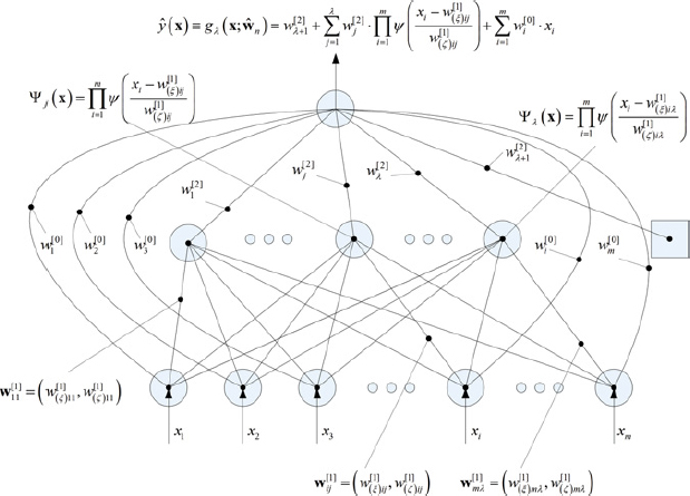
Figure 3.1 Feedforward wavelet neural network.
The structure of a single-hidden-layer feedforward wavelet network is given in Figure 3.1. The network output is given by the expression
where Ψj(x) is a multidimensional wavelet constructed by the product of m scalar wavelets, x the input vector, m the number of network inputs, λ the number of hidden units, and w a network weight. The multidimensional wavelets are computed as follows:
where ψ is the mother wavelet and
In the expression above, i = 1, …, m, j = 1, …, λ + 1, and the weights w correspond to the translation (w[1](ξ)ij) and the dilation (w[1](ζ)ij) factors. The complete vector of the network parameters comprises w = (w[0]i, wj[2], w[2]λ + 1, w(ξ)ij[1], w[1](ζ)ij). These parameters are adjusted during the training phase.
In the literature, three mother wavelets are usually suggested: the Gaussian derivative, given by
the second derivative of the Gaussian, the Mexican hat,
and the Morlet wavelet, given by
Selection of the mother wavelet depends on the application and is not limited to the foregoing choices. The activation function can be a wave net (orthogonal wavelets) or a wave frame (continuous wavelets). Following Becerikli et al. (2003), Billings and Wei (2005), and Zhang (1994), we use as a mother wavelet the Mexican hat function, which proved to be useful and to work satisfactorily in various applications.
Initialization of the Parameters of the Wavelet Network
In wavelet networks, in contrast to neural networks that use sigmoid functions, selecting initial values of the dilation and translation parameters randomly may not be suitable (Oussar et al., 1998). A wavelet is a waveform of effectively limited duration that has an average value of zero and localized properties; hence, a random initialization may lead to wavelons with a value of zero. Training algorithms such as gradient descent with random initialization are inefficient (Zhang, 1993), since random initialization affects the speed of training and may lead to a local minimum of the loss function (Postalcioglu and Becerikli, 2007). Also, in sigmoid neural networks, although a minimization of the loss function can be replicated with random initialization, the values of the weights will vary each time (Anders and Korn, 1999).
Utilizing the information that can be extracted by wavelet analysis from the input data set, the initial values of the parameters w of the network can be selected in an efficient way. Efficient initialization will result in fewer iterations in the training phase of the network and training algorithms that will avoid local minimums of the loss function in the training phase. Finally, efficient initialization methods will approximate the same vector of weights that minimize the loss function each time.
Various methods have been proposed for optimized initialization of the wavelet parameters. In the rest of the chapter the following methods are discussed: the heuristic, residual-based selection (RBS), selection by orthogonalization (SSO), and backward elimination (BE).
The Heuristic Initialization Method
The following initialization for the translation and dilation parameters was introduced by Zhang and Benveniste (1992):
where Mi and Ni are defined as the maximum and minimum of input xj:
In the framework above, the initialization of the parameters is based on the input domains defined by examples of the training sample (Oussar et al., 1998). In other words, the center of the wavelet j is initialized at the center of the parallelepiped defined by the input domain. These initializations guarantee that the wavelets extend initially over the entire input domain (Oussar and Dreyfus, 2000). This procedure is very simple and the computational burden is almost negligible. Initialization of the direct connections w[0]i and the weights w[2]j is less important, and they are initialized in small random values between 0 and 1.
Complex Initialization Methods
The previous heuristic method is simple and its computational cost is almost negligible. However, it is not efficient, as shown on the next section. The heuristic method does not guarantee that the training will find the global minimum. Moreover, this method does not use any information that the wavelet decomposition can provide.
Recent studies proposed more complex methods that utilize the information extracted by wavelet analysis (Kan and Wong, 1998; Oussar and Dreyfus, 2000; Oussar et al., 1998; Wong and Leung, 1998; Xu and Ho, 2002; Zhang, 1997). These methods are not optimal, simply a trade-off between optimality and efficiency (He et al., 2002). Implementation of these methods can be summed up in the following three steps:
- Construct a library W of wavelets.
- Remove the wavelets whose support does not contain any sample points of the training data.
- Rank the remaining wavelets and select the best wavelet regressors.
In the first step, the wavelet library can be constructed by either an orthogonal wavelet or a wavelet frame (He et al., 2002; Postalcioglu and Becerikli, 2007). By determining an orthogonal wavelet basis, the wavelet network is constructed simultaneously. However, to generate an orthogonal wavelet basis, the wavelet function has to satisfy strong restrictions (Daubechies, 1992; Mallat, 1999). In addition, the fact that orthogonal wavelets cannot be expressed in closed form makes them inappropriate for applications of function approximation or process modeling (Oussar and Dreyfus, 2000).
On the other hand, constructing wavelet frames is very easy and can be done by translating and dilating the mother wavelet selected. Results from Gao and Tsoukalas (2001) indicate that a family of compactly supported nonorthogonal wavelets is more appropriate for function approximation. Due to the fact that a wavelet family can contain a large number of wavelets, it is more convenient to use a truncated wavelet family than an orthogonal wavelet basis (Zhang, 1993).
However, constructing a wavelet network using wavelet frames is not a straightforward process. The wavelet library may contain a large number of wavelets since only the input data were considered in construction of the wavelet frame. To construct a wavelet network, the “best” wavelets must be selected. To do so, first the number of wavelet candidates must be decreased and the remaining wavelets must be ranked. The reduction of the wavelet candidates must be done carefully since arbitrary truncations may lead to large errors (Xu and Ho, 2005). In the second step, Zhang (1993) proposes removing wavelets that have very few training patterns in their support. Alternatively, magnitude-based methods were used by Cannon and Slotine (1995) to eliminate wavelets with small coefficients. In the third step, the remaining wavelets are ranked and the wavelets with the highest rank are used for construction of the wavelet network.
In the next section, three alternative methods are presented to reduce and rank the wavelets in the wavelet library: residual-based selection, stepwise selection by orthogonalization, and backward elimination.
Residual-Based Selection Initialization Method
In the framework of RBS, the wavelet that best fits the output data is selected first. Then the wavelet that best fits the residual of the fitting of the preceding stage is selected repeatedly. RBS is considered to be a very simple method but not an effective one (Juditsky et al., 1994). However, if the wavelet candidates reach a very large number, computational efficiency is essential and the RBS method may be used (Juditsky et al., 1994). Kan and Wong (1998) and Wong and Leung (1998) used the RBS algorithm for the synthesis of wavelet networks. Xu and Ho (2002) used a modified version of the RBS algorithm. An orthogonalized residual-based selection (ORBS) algorithm is proposed for more precise initialization of the wavelet network. The ORBS method combines the RBS and orthogonalized least squares (OLS) method. In this way, high efficiency is obtained while relatively low computational burden is maintained.
Selection by Orthogonalization Method
The RBS method does not explicitly consider the interaction or nonorthogonality of the wavelets in the wavelet basis (Zhang, 1997). The SSO method is an extension of the RBS first proposed by Chen et al. (1989, 1991). The following procedure is followed to initialize the wavelet network: First, the wavelet that best fits the output data is selected. Then the wavelet that best fits the residual of the fitting of the previous stage together with the wavelet selected previously is selected repeatedly. In other words, the SSO considers the interaction or nonorthogonality of the wavelets. The selection of the wavelets is performed using the modified Gram–Schmidt algorithm, which has better numerical properties and is computationally less expensive than the ordinary Gram–Schmidt algorithm (Zhang, 1997). More precisely, the modified Gram–Schmidt algorithm is applied with a particular choice of the order in which the vectors are orthogonalized. SSO is considered to have good efficiency while not being expensive computationally. An algorithm similar to SSO was proposed by Oussar and Dreyfus (2000).
gram–schmidt algorithm
The ranking method adopted here is the Gram–Schmidt procedure. The algorithm has been presented in detail by Chen et al. (1989). In this section the basic aspects of the algorithm are presented briefly. The basic problem that we want to solve is the following: Suppose that ![]() is a linear independent set of vectors. How do we find an orthonormal set of vectors {q1, q2, …, qk} with the property span{q1, q2, …, qk} = span{x1, x2, …, xk}?
is a linear independent set of vectors. How do we find an orthonormal set of vectors {q1, q2, …, qk} with the property span{q1, q2, …, qk} = span{x1, x2, …, xk}?
A set of vectors are called orthonormal if the following two conditions are met:
Equation (3.11) ensures that the vectors qi are orthogonal and (3.12) that they are normalized. Consider a model, linear with respect to its parameters, with k inputs and a training set of n training patterns. The inputs are ranked as follows. First, the input vector that has the smallest angle with the vector output is selected. Then all other input vectors, and the output vector, are projected onto the subspace orthogonal to the input vector selected. In this subspace of dimension k − 1, the procedure is iterated, and it is terminated when all inputs are ranked. That is, at step j the jth column is made orthogonal to each of the j − 1 columns orthogonalized previously, and the operations are repeated for j = 2, …, k.
Since the output of the wavelet network is linear with respect to the weights, the procedure described above can easily be used where each input is actually the output of a multidimensional wavelet. Therefore, at the end of the procedure, all the wavelets of the library are ranked. The part of the process output not yet modeled and the wavelets not yet selected are subsequently projected onto the subspace orthogonal to the regressor selected. The procedure is repeated until all wavelets are ranked.
It is well known that the Gram–Schmidt procedure is very sensitive to round-off errors (Chen et al., 1989). It has been proved that if the regression matrix is ill-conditioned, the orthogonality will be lost. On the other hand, the modified Gram–Schmidt procedure is numerically stable. In this procedure, at the jth stage the columns subscripted j + 1, …, k are made orthogonal to the jth column and the operations repeated for j = 1, …, k − 1. Both methods perform basically the same operations, only in a different sequence. However, the two algorithms have distinct differences in computational behavior. The modified procedure is more accurate and more stable than the classical algorithm. In all simulations presented below we have used the modified Gram–Schmidt method.
The algorithm can be summarized in the following two steps. At step 1 we must compute the orthogonal vectors {z1, …, zk}. Hence, we set
At step 2 the vectors {z1, …, zk} are normalized:
Backward Elimination Method
In contrast to previous methods, the BE starts the regression by selecting all available wavelets from the wavelet library. The wavelet that contributes the least in the fitting of the training data is repeatedly eliminated. The objective is to increase the residual at each stage as little as possible. The drawback of BE is that it is computationally expensive, but it is considered to have good efficiency.
Zhang (1997) presented the exact number of arithmetic operations for each algorithm. More precisely, for the RSO at each step i the computational cost is 2nL − 2in + 6n − 1, where n is the length of the training samples and L is the number of wavelets in the wavelet basis. Similarly, the computational cost of the SSO algorithm at each step is 8nL − 6in + 9n + 5L. Roughly speaking, the SSO is four times more computationally expensive than the RSO algorithm. Finally, the operations needed in the BE method is 2n(L − i) + 4(L2 + i2) − 8iL − (L − i). In addition, at the beginning of the BE algorithm an L × L matrix must be inverted. If the number of hidden units, and as a result the number of wavelets that must be selected is ![]() , fewer steps are performed by the BE algorithm, whereas for
, fewer steps are performed by the BE algorithm, whereas for ![]() the contrary is true (Zhang, 1997).
the contrary is true (Zhang, 1997).
All methods described above are used only for the initialization of the dilation and translation parameters. The network is trained further to obtain the vector of the parameters ![]() , which minimizes the cost function. It is clear that additional computational burden is added to initialize the wavelet network efficiently. However, the efficient initialization significantly reduces the training phase; hence, the total number of computations is significantly smaller than in a network with random initialization.
, which minimizes the cost function. It is clear that additional computational burden is added to initialize the wavelet network efficiently. However, the efficient initialization significantly reduces the training phase; hence, the total number of computations is significantly smaller than in a network with random initialization.
Training a Wavelet Network with Backpropagation
After the initialization phase, the network is trained further to find the weights that minimize the cost function. As wavelet networks have gained in popularity, more complex training algorithms have been presented in the literature. Cristea et al. (2000) used genetic algorithms to train a wavelet network; Li and Chen (2002) proposed a learning algorithm that utilized least trimmed squares. He et al. (2002) suggest a hierarchical evolutionary algorithm. Xu and Ho (2005) employed the Levenberg–Marquardt algorithm. Chen et al. (2006) combine adaptive diversity learning particle swarm optimization and gradient descent algorithms to train a wavelet network. However, most evolutionary algorithms that include particle swarm optimization are inefficient and cannot avoid completely certain degeneracy and local minimum (Zhang, 2009). Also, evolutionary algorithms suffer from fine-tuning inefficiency (Chen et al., 2006; Yao, 1999). On the other hand, the Levenberg–Marquardt is one of the fastest algorithms for training classical sigmoid neural networks. The main drawback of this algorithm is that it requires the storage and inversion of some matrices that can be quite large.
The algorithms above originate from classical sigmoid neural networks, as they do not take advantage of the properties of wavelets (Zhang, 2007, 2009). Since a wavelet is a function whose energy is well localized in time frequency, Zhang (2007, 2009) used sampling theory to train a wavelet network in both uniform and nonuniform data. Their results indicate that the algorithm they proposed has global convergence.
In our implementation, ordinary backpropagation (BP) was used. Backpropagation is probably the most popular algorithm used for training wavelet networks (Fang and Chow, 2006; Jiao et al., 2001; Oussar and Dreyfus, 2000; Oussar et al., 1998; Postalcioglu and Becerikli, 2007; Zhang, 1997, 2007; Zhang and Benveniste, 1992). Ordinary BP is less fast but also less prone to sensitivity to initial conditions than are higher-order alternatives (Zapranis and Refenes, 1999).
The basic idea of backpropagation is to find the percentage contribution of each weight to the error. The error ep for pattern p is simply the difference between the target (yp) and the network output (![]() ). By squaring and multiplying by ½, we take the pairwise error Ep, which is used in network training:
). By squaring and multiplying by ½, we take the pairwise error Ep, which is used in network training:
The weights of the network were trained to minimize the mean quadratic cost function (or loss function):
Other functions can be used instead of (3.14); however, the mean quadratic cost function is the most commonly used. The network is trained until a vector of weights ![]() that minimizes the proposed cost function is found. The previous solution corresponds to a training sample of size n. Computing the parameter vector
that minimizes the proposed cost function is found. The previous solution corresponds to a training sample of size n. Computing the parameter vector ![]() is always done by iterative methods. At each iteration t the derivative of the loss function with respect to the network weights is calculated. Then the parameters are updated using the following (delta) learning rule:
is always done by iterative methods. At each iteration t the derivative of the loss function with respect to the network weights is calculated. Then the parameters are updated using the following (delta) learning rule:
where η is the learning rate and it is constant. The complete vector of the network parameters comprises w = (w[0]i, w(ξ)ij[1], w[1](ζ)ij, wj[2], w[2]λ + 1).
A constant momentum term, defined by κ, is induced which increases the training speed and helps the algorithm to avoid oscillations. The learning rate and momentum speed take values between 0 and 1. Choice of the learning rate and the momentum depend on the application and the training sample. Usually, values between 0.1 and 0.4 are used.
The partial derivative of the cost function with respect to a weight w is given by
The partial derivatives with respect to each parameter ![]() , and with respect to each input variable
, and with respect to each input variable ![]() , are presented below. The partial derivative with respect to (w.r.t.) the bias term w[2]λ + 1 is given by
, are presented below. The partial derivative with respect to (w.r.t.) the bias term w[2]λ + 1 is given by

Similarly, the partial derivatives w.r.t. the direct connections from the input variables w[0]i to the output of the wavelet network ![]() are given by
are given by
The partial derivatives w.r.t. the linear connections from the wavelons w[2]j to the output of the wavelet network are given by
The partial derivatives w.r.t. the translation w[1](ξ)ij are given by
The partial derivatives w.r.t. the dilation parameters w[1](ζ)ij are given by
Finally, the partial derivatives w.r.t. the input variables ![]() are presented:
are presented:
The partial derivatives ![]() are needed for the variable selection algorithm that is presented in the following chapters.
are needed for the variable selection algorithm that is presented in the following chapters.
Online Training
The training methodology described above falls into the category of off-line training. This means that the weights of the networks are updated after all training patterns are presented to the network. Alternatively, one can use online training methods. In online methods the weights are changed after each presentation of a training pattern. For some problems, this method may yield effective results, especially for problems where data arrive in real time (Samarasinghe, 2006). Using online training it is possible to reduce training times significantly. However, for complex problems it is possible that online training will create a series of drawbacks. First, there is the possibility that the training will stop before the presentation of each training pattern to the network. Second, by changing the weights after each pattern, they could bounce back and forth with each iteration, possibly resulting in a substantial amount of wasted time (Samarasinghe, 2006). Hence, to ensure the stability of the algorithms, off-line training is used in this book.
Stopping Conditions for Training
After the initialization phase of the network parameters w, the weights w[0]i and w[2]j and the parameters w[1](ξ)ij and w[1](ζ)ij are trained during the learning phase for approximating the target function. A key decision related to the training of a wavelet network involves when the weight adjustment should end. If the training phase stops early, the wavelet network will not be able to learn the underlying function of the training data and as a result will not perform well in predicting new, unseen data. On the other hand, if the training phase continues beyond the appropriate iterations, the network will begin to learn the noise part of the data and will become overfitted. As a result, the generalization ability of the network will be lost. Hence, it will not be appropriate to use the wavelet network in predicting future data.
In the next section a procedure for selecting the correct topology of a wavelet network is presented. Under the assumption that the wavelet network contains the number of wavelets that minimizes the prediction risk, the training is stopped when one of the following criteria is met: The cost function reaches a fixed lower bound or the variations of the gradient, the variations of the parameters reach a lower bound, or the number of iterations reaches a fixed maximum, whichever is satisfied first. In our implementation the fixed lower bound of the cost function, of the variations of the gradient, and of the variations of the parameters were set to 10− 5.
Evaluating the Initialization Methods
As mentioned earlier, the initialization phase is very important to the construction and training of a wavelet network. In this section we compare four different initialization methods: the heuristic, SSO, RBS, and BE methods, which constitute the bases for alternative algorithms and can be used with the BP training algorithm. The four initialization methods will be compared in three stages. First, the distance between the initialization and the underlying function as well as the training data will be measured. Second, the number of iterations needed to train the wavelet network will be compared. Finally, the difference between the final approximation of the trained wavelet network and the underlying function and the training data will be examined. The four initialization methods will be tested in two cases: on a simple underlying function and on a more complex function that incorporates large outliers.
Case 1: Sinusoid and Noise with Decreasing Variance
In the first case the underlying function f(x) is given by
where x is equally spaced in [0,1] and the noise ϵ1(x) follows a normal distribution with mean zero and decreasing variance:
The four initialization methods are examined using a wavelet network with 2 hidden units with learning rate 0.1 and momentum 0. The choice of the network structure proposed will be justified in Chapter 4. The training sample consists of 1.000 patterns.
Figure 3.2 shows the initialization of the four algorithms for the first training sample. It is clear that the heuristic algorithm produces the worst initialization. However, even the heuristic approximation is still better than a random initialization. On the other hand, initialization of the RBS algorithm gives a better approximation of the data; however, the approximation of the target function f(x) is still not very good. Finally, both the SSO and BE algorithms start very close to the target function f(x). For the construction of the wavelet basis, the input dimension was scanned in four scale levels and 15 wavelet candidates were identified. To reduce the number of wavelet candidates, wavelets that contain fewer than three patterns in their support are removed from the basis. However, all wavelets contain at least three training samples; hence, the wavelet basis was not truncated.
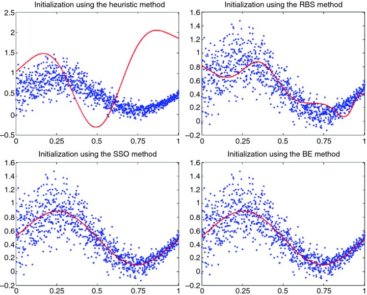
Figure 3.2 Four different initialization methods in the first case.
The mean squared error (MSE) between the initialization of the network and the training data confirms the results cited above. More precisely, the MSE between the initialization of the network and the training data is 0.630809, 0.040453, 0.031331, and 0.031331 for the heuristic, RBS, SSO, and BE, respectively. Next we test how close the initialization is to the underlying function. The MSE between the initialization of the network and the underlying function is 0.59868, 0.302782, 0.000121, and 0.000121 for the heuristic, RBS, SSO, and BE, respectively. The results above indicate that the SSO and the BE produce the best initialization for the parameters of the wavelet network.
Another way to compare the initialization methods is to compare the number of iterations needed in the training phase until the solution ![]() is found. Also, whether or not the initialization methods proposed allows the training procedure to find the global minimum of the loss function will be examined.
is found. Also, whether or not the initialization methods proposed allows the training procedure to find the global minimum of the loss function will be examined.
The heuristic method was used to train 100 networks with different initial conditions for the direct connections w[0]i and weights w[2]j. Training 100 networks with perturbed initial conditions is expected to be sufficient to avoid any possible local minimums of the loss function (3.14). It was found that the smallest MSE between the target function f(x) and the final approximation of the network was 0.031331.
Using the RBS, the training phase stopped after 616 iterations. The overall fit was very good and the MSE between the network output and the training data was 0.031401, indicating that the network was stopped before the minimum of the loss function was achieved. Finally, the MSE between the network output and the target function was 0.000676.
On the other hand, when initializing the wavelet network with the SSO algorithm, only one iteration was needed in the training phase and the MSE was 0.031331, whereas the MSE between the underlying function f(x) and the network approximation was only 0.000121. The same results were achieved using the BE method. Finally, one implementation of the heuristic method needed 1501 iterations. The results are presented in Table 3.1.
Table 3.1 Initialization of the Four Methodsa
| Heuristic | RBS | SSO | BE | |
| Case 1 | ||||
| MSE | 0.031522 | 0.031401 | 0.031331 | 0.031331 |
| MSE+ | 0.000791 | 0.000626 | 0.000121 | 0.000121 |
| IMSE | 0.630807 | 0.040453 | 0.031331 | 0.031331 |
| IMSE+ | 0.598680 | 0.302782 | 0.000121 | 0.000121 |
| Iterations | 1501 | 616 | 1 | 1 |
| Case 2 | ||||
| MSE | 0.106238 | 0.004730 | 0.004752 | 0.004364 |
| MSE+ | 0.102569 | 0.000558 | 0.000490 | 0.000074 |
| IMSE | 7.877472 | 0.041256 | 0.012813 | 0.008403 |
| IMSE+ | 7.872084 | 0.037844 | 0.008394 | 0.004015 |
| Iterations | 4433 | 3097 | 751 | 1107 |
aCase 1 refers to function f(x) and case 2 to function g(x). RBS, residual-based selection; SSO, stepwise selection by orthogonalization; BE, backward elimination; MSE, MSE between the training data and the network approximation; MSE+, MSE between the underlying function and the network approximation; IMSE, MSE between the training data and the network initialization; IMSE+, MSE between the underlying function and the network initialization.
The results above indicate that the SSO and BE algorithms give the same results and significantly outperform both the heuristic and RBS algorithms. Moreover, the results above indicate that having a very good initialization not only significantly reduces the needed training iterations and as a result the total needed training time, but a vector of weights ![]() that minimizes the loss function can also be found.
that minimizes the loss function can also be found.
Case 2: Sum of Sinusoids and Cauchy Noise
Next, a more complex case is introduced where the function g(x) is given by
and ϵ2(x) follows a Cauchy distribution with location 0 and scale 0.05, and x is equally spaced in [−6, 6]. The training sample consists of 1.000 training patterns. Whereas the first function is very simple, the second one, proposed by Li and Chen (2002), incorporates large outliers in the output space. The sensitivity to the presence of outliers of the wavelet network proposed will be tested. To approximate function g(x), a wavelet network with 8 hidden units with learning rate 0.1 and momentum 0 is used. The choice of the topology proposed for the wavelet network is justified in Chapter 4.
The results obtained in the second case are similar. A closer inspection of Figure 3.3 reveals that the heuristic algorithm produces the worst initialization in approximating the underlying function g(x). The RBS algorithm produces a significantly better initialization than the heuristic method; however, the initial approximation still differs from the training target values. Finally, both the BE and SSO algorithms produce a very good initialization. It is clear that the first approximation of the wavelet network is very close to the underlying function g(x).
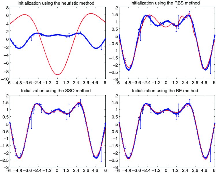
Figure 3.3 Four initialization methods for the second case.
For construction of the wavelet basis, the input dimension was scanned in depth at five scale levels. The analysis revealed 31 wavelet candidates, and all of them were used for construction of the wavelet basis since all of them had at least three training samples in their support. The MSE between the initialization of the network and the training data was 7.87472, 0.041256, 0.012813, and 0.008403 for the heuristic, RBS, SSO, and BE algorithms, respectively. Also, the MSE between the initialization of the network and the underlying function g(x) was 7.872084, 0.037844, 0.008394, and 0.004015 for the heuristic, RBS, SSO, and BE, respectively. The previous results indicate that the training phase using the BE algorithm starts very close to the target function g(x).
Next, the number of iterations needed in the training phase of each method was compared. Also, whether or not the initialization methods proposed allow the training procedure to find the global minimum of the loss function was examined. The RBS algorithm stopped after 3097 iterations, and the MSE of the final approximation of the wavelet network and the training patterns was 0.004730. The MSE between the underlying function f(x) and the network approximation was 0.000558. When initializing the wavelet network with the SSO algorithm only, 741 iterations were needed in the training phase and the MSE was 0.004752, while the MSE between the underlying function g(x) and the network approximation was 0.000490. The BE needed 1107 iterations in the training phase and the MSE was 0.004364, while the MSE between the underlying function g(x) and the network approximation was only 0.000074. Finally, one implementation of the heuristic method needed 4433 iterations and the MSE was 0.106238, while the MSE between the underlying function g(x) and the network approximation was 0.102569. The results are presented in the second part of Table 3.1. In the second case the BE was slower than the SSO; however, the final approximation was significantly closer to the target function than with any other method. Note that in all cases the training was stopped when the minimum velocity, 10− 5, was reached. If the minimum velocity is reduced further, the SSO algorithm will produce results similar to those of the BE, but extra computational time will be needed.
The previous examples indicate that the SSO and BE perform similarly and outperform the other two methods, whereas BE outperforms the SSO in complex problems. Previous studies suggest that the BE is more efficient than the SSO algorithm; however, it is more computationally expensive. On the other hand, in the BE algorithm it is necessary to calculate the inverse of the wavelet matrix, whose columns might be linearly dependent (Zhang, 1997). In that case the SSO must be used. However, since the wavelets come from a wavelet frame, this happens very rarely (Zhang, 1997).
Conclusions
In this chapter the structure of the wavelet network proposed was presented and discussed analytically. A wavelet network usually has the form of a three-layer network. The lower layer represents the input layer, the middle layer is the hidden layer, and the upper layer is the output layer. In our implementation, a multidimensional wavelet network with a linear connection between the wavelons and the output is utilized. In addition, there are direct connections from the input layer to the output layer that will help the network to perform well in linear applications.
Furthermore, the initialization phase, training phase, and stopping conditions are discussed. The initialization of the parameters is very important in wavelet networks since it can reduce the training time significantly. The initialization method developed extracts useful information from the wavelet analysis. The simplest method is the heuristic method; more sophisticated methods, such as residual-based selection, selection by orthogonalization, and backward elimination can be used for efficient initialization.
The results from our analysis indicate that backward elimination significantly outperforms other methods. The results from two simulated cases show that using the backward elimination method, the wavelet network provides a fit very close to the real underlying function. However, it is more computationally expensive than the other methods.
The backpropagation method is used for network training. Iteratively, the weights of the networks are updated based on the delta learning rule, where a learning rate and a momentum are used. The weights of the network were trained to minimize the mean quadratic cost function. The training continues until one of the stopping conditions is met.
References
- Anders, U., and Korn, O. (1999). “Model selection in neural networks.” Neural Networks, 12(2), 309–323.
- Becerikli, Y. (2004). “On three intelligent systems: dynamic neural, fuzzy and wavelet networks for training trajectory.” Neural Computation and Applications, 13, 339–351.
- Becerikli, Y., Oysal, Y., and Konar, A. F. (2003). “On a dynamic wavelet network and its modeling application.” Lecture Notes in Computer Science, 2714, 710–718.
- Billings, S. A., and Wei, H.-L. (2005). “A new class of wavelet networks for nonlinear system identification.” IEEE Transactions on Neural Networks, 16(4), 862–874.
- Cannon, M., and Slotine, J.-J. E. (1995). “Space–frequency localized basis function networks for nonlinear system estimation and control.” Neurocomputing, 9, 293–342.
- Chen, Y., Billings, S. A., and Luo, W. (1989). “Orthogonal least squares methods and their application to non-linear system identifcation.” International Journal of Control, 50, 1873–1896.
- Chen, Y., Cowan, C., and Grant, P. (1991). “Orthogonal least squares learning algorithm for radial basis function networks.” IEEE Transactions On Neural Networks, 2, 302–309.
- Chen, Y., Yang, B., and Dong, J. (2006). “Time-series prediction using a local linear wavelet neural wavelet.” Neurocomputing, 69, 449–465.
- Cristea, P., Tuduce, R., and Cristea, A. (2000). “Time series prediction with wavelet neural networks.” Proceedings of 5th Seminar on Neural Network Applications in Electrical Engineering, Belgrade, Yugoslavia, 5–10.
- Daubechies, I. (1992). Ten Lectures on Wavelets. SIAM, Philadelphia.
- Fang, Y., and Chow, T. W. S. (2006). “Wavelets based neural network for function approximation.” Lecture Notes in Computer Science, 3971, 80–85.
- Gao, R., and Tsoukalas, H. I. (2001). “Neural-wavelet methodology for load forecasting.” Journal of Intelligent and Robotic Systems, 31, 149–157.
- He, Y., Chu, F., and Zhong, B. (2002). “A hierarchical evolutionary algorithm for constructing and training wavelet networks.” Neural Computing and Applications, 10, 357–366.
- Jiao, L., Pan, J., and Fang, Y. (2001). “Multiwavelet neural network and its approximation properties.” IEEE Transactions on Neural Networks, 12(5), 1060–1066.
- Juditsky, A., Zhang, Q., Delyon, B., Glorennec, P.-Y., and Benveniste, A. (1994). “Wavelets in identification—wavelets, splines, neurons, fuzzies: how good for identification?” Techincal Report, INRIA.
- Kadambe, S., and Srinivasan, P. (2006). “Adaptive wavelets for signal classification and compression.” International Journal of Electronics and Communications, 60, 45–55.
- Kan, K.-C., and Wong, K. W. (1998). “Self-construction algorithm for synthesis of wavelet networks.” Electronic Letters, 34, 1953–1955.
- Khayamian, T., Ensafi, A. A., Tabaraki, R., and Esteki, M. (2005). “Principal component-wavelet networks as a new multivariate calibration model.” Analytical Letters, 38(9), 1447–1489.
- Li, S. T., and Chen, S.-C. (2002). “Function approximation using robust wavelet neural networks.” Proceedings of ICTAI ’02, Washington, DC, 483–488.
- Mallat, S. G. (1999). A Wavelet Tour of Signal Processing. Academic Press, San Diego, CA.
- Mellit, A., Benghamen, M., and Kalogirou, S. A. (2006). “An adaptive wavelet-network model for forecasting daily total solar-radiation.” Applied Energy, 83, 705–722.
- Oussar, Y., and Dreyfus, G. (2000). “Initialization by selection for wavelet network training.” Neurocomputing, 34, 131–143.
- Oussar, Y., Rivals, I., Presonnaz, L., and Dreyfus, G. (1998). “Trainning wavelet networks for nonlinear dynamic input output modelling.” Neurocomputing, 20, 173–188.
- Postalcioglu, S., and Becerikli, Y. (2007). “Wavelet networks for nonlinear system modelling.” Neural Computing and Applications, 16, 434–441.
- Samarasinghe, S. (2006). Neural Networks for Applied Sciences and Engineering. Taylor & Francis Group, New York.
- Wong, K.-W., and Leung, A. C.-S. (1998). “On-line successive synthesis of wavelet networks.” Neural Processing Letters, 7, 91–100.
- Xu, J., and Ho, D. W. C. (1999). “Adaptive wavelet networks for nonlinear system identification.” Proceedings of American Control Conference, San Diego, CA.
- Xu, J., and Ho, D. W. C. (2002). “A basis selection algorithm for wavelet neural networks.” Neurocomputing, 48, 681–689.
- Xu, J., and Ho, D. W. C. (2005). “A constructive algorithm for wavelet neural networks.” Lecture Notes in Computer Science, 3610, 730–739.
- Yao, X. (1999). “Evolving artificial neural networks.” Proceedings IEEE, 87(9), 1423–1447.
- Zapranis, A., and Refenes, A. P. (1999). Principles of Neural Model Indentification, Selection and Adequacy: With Applications to Financial Econometrics. Springer-Verlag, New York.
- Zhang, Q. (1993). “Regressor selection and wavelet network construction.” Technical Report, INRIA.
- Zhang, Q. (1994). “Using Wavelet Network in Nonparametric Estimation.” Technical Report, 2321, INRIA.
- Zhang, Q. (1997). “Using wavelet network in nonparametric estimation.” IEEE Transactions on Neural Networks, 8(2), 227–236.
- Zhang, Q., and Benveniste, A. (1992). “Wavelet networks.” IEEE Transactions on Neural Networks, 3(6), 889–898.
- Zhang, Z. (2007). “Learning algorithm of wavelet network based on sampling theory.” Neurocomputing, 71(1), 224–269.
- Zhang, Z. (2009). “Iterative algorithm of wavelet network learning from nonuniform data.” Neurocomputing, 72, 2979–2999.
- Zhao, J., Chen, B., and Shen, J. (1998). “Multidimensional non-orthogonal wavelet-sigmoid basis function neural network for dynamic process fault diagnosis.” Computers and Chemical Engineering, 23, 83–92.