Chapter 7
Solutions for Power Quality Issues of Wind Generator Systems
7.1 Introduction
Using wind power to generate electricity is receiving more and more attention every day all over the world. One of the simplest methods of running a wind generation system is to use an induction generator (IG) connected directly to the power grid, because induction generators are the most cost-effective and robust machines for energy conversion. However, induction generators require reactive power for magnetization, particularly during startup. As the reactive power drained by the induction generators is coupled to the active power generated by them, the variability of wind speed results in variations of induction generators’ real and reactive powers. It is this variation in active and reactive powers that interacts with the network and provokes voltage and frequency fluctuations. These fluctuations cause lamp flicker and inaccuracy in the timing devices. If good penetration of the wind power is to be achieved, some remedial measures must be taken for power quality improvement. Since both frequency and voltages are often affected in these systems, fast-acting control devices (i.e., the energy storage devices) capable of exchanging active as well as reactive powers are appropriate candidates to meet this end. This chapter discusses various energy storage devices, comparison among them, and the use of energy storage devices in minimizing fluctuations in line power, frequency, and terminal voltage of wind generator systems. Furthermore, this chapter discusses the output power leveling of wind generator systems by pitch angle control, power quality improvement by flywheel energy storage system, and constant power control of doubly fed induction generator (DFIG) wind turbines with supercapacitor energy storage.
7.2 Various Energy Storage Systems
Various promising energy storage systems are available on the market battery, such as energy storage, supercapacitor energy storage, superconducting magnetic energy storage (SMES), flywheel energy storage, and compressed air energy storage [1].
Electrical energy in an alternating current (AC) system cannot be stored electrically. However, energy can be stored by converting the AC electricity and storing it electromagnetically, electrochemically, or kinetically or as potential energy. Each energy storage technology usually includes a power conversion unit to change the energy from one form to another. Two factors characterize the application of an energy storage technology. One is the amount of energy that can be stored in the device. This is a characteristic of the storage device itself. Another is the rate at which energy can be transferred into or out of the storage device. This depends mainly on the peak power rating of the power conversion unit but is also impacted by the response rate of the storage device itself. The power–energy ranges for near-to-midterm technologies are projected in Figure 7.1. Integration of these four possible energy storage technologies with flexible AC transmission systems (FACTS) and custom power devices are among the possible power applications of energy storage. The possible benefits include transmission enhancement, power oscillation damping, dynamic voltage stability, tie line control, short-term spinning reserve, load leveling, under-frequency load shedding reduction, circuit-breaker reclosing, subsynchronous resonance damping, and power quality improvement.
7.2.1 Superconducting Magnetic Energy Storage
Although superconductivity was discovered in 1911, it was not until the 1970s that SMES was first proposed as an energy storage technology for power systems. SMES systems have attracted the attention of both electric utilities and the military due to their fast response and high efficiency; they have a charge–discharge efficiency over 95%. Possible applications include load leveling, dynamic stability, transient stability, voltage stability, frequency regulation, transmission capability enhancement, and power quality improvement [1].

Figure 7.1 Specific power versus specific energy ranges for near-to-midterm technology.
When compared with other energy storage technologies, today’s SMES systems are still costly. However, the integration of an SMES coil into existing FACTS devices eliminates what is typically the largest cost for the entire SMES system—the inverter unit. Some studies have shown that micro (0.1 MWh) and midsize (0.1–100 MWh) SMES systems could potentially be more economical for power transmission and distribution applications. The use of high-temperature superconductors should also make SMES cost-effective due to reductions in refrigeration needs. There are a number of ongoing SMES projects currently installed or in development throughout the world.
An SMES unit is a device that stores energy in the magnetic field generated by the direct current (DC) current flowing through a super-conducting coil. The inductively stored energy (E in joules) and the rated power (P in watts) are commonly given specifications for SMES devices, and they can be expressed as follows:
where L is the inductance of the coil, I is the DC current flowing through the coil, and V is the voltage across the coil. Since energy is stored as circulating current, energy can be drawn from an SMES unit with almost instantaneous response with energy stored or delivered over periods ranging from a fraction of a second to several hours.
An SMES unit consists of a large superconducting coil at the cryogenic temperature. This temperature is maintained by a cryostat or dewar that contains helium or nitrogen liquid vessels. A power conversion/conditioning system (PCS) connects the SMES unit to an AC power system, and it is used to charge and discharge the coil. Two types of power conversion systems are commonly used. One option uses a current source converter (CSC) to both interface to the AC system and charge and discharge the coil. The second option uses a voltage source converter (VSC) to interface to the AC system and a DC-to-DC chopper to charge and discharge the coil. The VSC and DC-to-DC chopper share a common DC bus. The components of an SMES system are shown in Figure 7.2. The modes of charge–discharge–standby are obtained by controlling the voltage across the SMES coil (Vcoil). The SMES coil is charged or discharged by applying a positive or negative voltage, Vcoil, across the superconducting coil. The SMES system enters a standby mode operation when the average Vcoil is zero, resulting in a constant average coil current, Icoil.

Figure 7.2 Components of a typical SMES system.
Several factors are taken into account in the design of the coil to achieve the best possible performance of an SMES system at the least cost. These factors may include coil configuration, energy capability, structure, and operating temperature. A compromise is made between each factor by considering the parameters of energy/mass ratio, Lorentz forces, and stray magnetic field and by minimizing the losses for a reliable, stable, and economic SMES system. The coil can be configured as a solenoid or a toroid. The solenoid type has been used widely due to its simplicity and cost-effectiveness, though the toroid coil designs were also incorporated by a number of small-scale SMES projects. Coil inductance (L) or PCS maximum voltage (Vmax) and current (Imax) ratings determine the maximum energy/power that can be drawn or injected by an SMES coil. The ratings of these parameters depend on the application type of SMES. The operating temperature used for a superconducting device is a compromise between cost and the operational requirements. Low-temperature superconductor devices (LTSs) are available now, whereas high-temperature superconductor devices are currently in the development stage. The efficiency and fast response capability (milliwatts/millisecond) of SMES systems have been and can be further exploited in applications at all levels of electric power systems. The potential utility applications have been studied since the 1970s. SMES systems have been considered for the following: (1) load leveling; (2) frequency support (spinning reserve) during loss of generation; (3) enhancing transient and dynamic stability; (4) dynamic voltage support (VAR compensation); (5) improving power quality; and (6) increasing transmission line capacity, thus enhancing overall reliability of power systems. Further development continues in power conversion systems and control schemes, evaluation of design and cost factors, and analyses for various SMES system applications. The energy and power characteristics for potential SMES applications for generation, transmission, and distribution are depicted in Figure 7.3. The square area in the figure represents the applications that are currently economical. Therefore, the SMES technology has a unique advantage in two types of application: power system transmission control; and stabilization and power quality.

Figure 7.3 Energy–power characteristics of potential SMES applications.
The cost of an SMES system can be separated into two independent components: (1) the cost of the energy storage capacity; and (2) the cost of the power handling capability. Storage-related cost includes the capital and construction costs of the conductor, coil structure components, cryogenic vessel, refrigeration, protection, and control equipment. Power-related cost involves the capital and construction costs of the power conditioning system. While the power-related cost is lower than the energy-related cost for large-scale applications, it is more dominant for small-scale applications.
7.2.2 Battery Energy Storage Systems
Batteries are one of the most cost-effective energy storage technologies available, with energy stored electrochemically. A battery system is made up of a set of low-voltage/power battery modules connected in parallel and series to achieve a desired electrical characteristic. Batteries are “charged” when they undergo an internal chemical reaction under a potential applied to the terminals. They deliver the absorbed energy, or “discharge,” when they reverse the chemical reaction. Key factors of batteries for storage applications include: high-energy density, high-energy capability, round-trip efficiency, cycling capability, life span, and initial cost.
There are a number of battery technologies under consideration for large-scale energy storage. Lead acid batteries represent an established, mature technology. Lead acid batteries can be designed for bulk energy storage or for rapid charge and discharge. Improvements in energy density and charging characteristics are still an active research area, with different additives under consideration. Lead acid batteries still represent a low-cost option for most applications requiring large storage capabilities; low-energy density and limited cycle life are the chief disadvantages. Mobile applications favor sealed lead acid battery technologies for safety and ease of maintenance. Valve-regulated lead acid (VRLA) batteries have better cost and performance characteristics for stationary applications. Several other battery technologies also show promise for stationary energy storage applications. All have higher energy density capabilities than lead acid batteries, but at present they are not yet cost-effective for higher-power applications. Leading technologies include nickel–metal– hydride batteries, nickel–cadmium batteries, and lithium–ion batteries. The last two technologies are both being pushed for electric vehicle applications where high-energy density can offset higher cost to some degree.
Due to the chemical kinetics involved, batteries cannot operate at high power levels for long time periods. In addition, rapid, deep discharges may lead to early replacement of the battery, since heating resulting in this kind of operation reduces battery lifetime. There are also environmental concerns related to battery storage due to toxic gas generation during battery charge and discharge. The disposal of hazardous materials presents some battery disposal problems. The disposal problem varies with battery technology. For example, the recycling and disposal of lead acid batteries is well established for automotive batteries. Batteries store DC charge, so power conversion is required to interface a battery with an AC system. Small, modular batteries with power electronic converters can provide four-quadrant operation (bidirectional current flow and bidirectional voltage polarity) with rapid response. Advances in battery technologies offer increased energy storage densities, greater cycling capabilities, higher reliability, and lower cost. Battery energy storage systems (BESSs) have recently emerged as one of the more promising near-term storage technologies for power applications, offering a wide range of power system applications such as area regulation, area protection, spinning reserve, and power factor correction. Several BESS units have been designed and installed in existing systems for the purposes of load leveling, stabilizing, and load frequency control. Optimal installation site and capacity of BESSs can be determined depending on their application. This has been done for load-leveling applications. Also, the integration of battery energy storage with a FACTS power flow controller can improve the power system operation and control.
7.2.3 Advanced Capacitors
Capacitors store electric energy by accumulating positive and negative charges (often on parallel plates) separated by an insulating dielectric. The capacitance, C, represents the relationship between the stored charge, q, and the voltage between the plates, V, as shown in (7.2). The capacitance depends on the permittivity of the dielectric, e, the area of the plates, A, and the distance between the plates, d, as shown in (7.3). Equation (7.4) shows that the energy stored on the capacitor depends on the capacitance and on the square of the voltage.
The amount of energy a capacitor is capable of storing can be increased by either increasing the capacitance or the voltage stored on the capacitor. The stored voltage is limited by the voltage-withstand-strength of the dielectric (which impacts the distance between the plates). Capacitance can be increased by increasing the area of the plates, increasing the permittivity, or decreasing the distance between the plates. As with batteries, the turnaround efficiency when charging and discharging capacitors is also an important consideration, as is response time. The effective series resistance (ESR) of the capacitor has a significant impact on both. The total voltage change when charging or discharging capacitors is shown in (7.5). Note that Ctot and Rtot are the result from a combined series/parallel configuration of capacitor cells to increase the total capacitance and the voltage level. The product CtotRtot determines the response time of the capacitor for charging or discharging.
Capacitors are used in many AC and DC applications in power systems. DC storage capacitors can be used for energy storage for power applications. They have long seen use in pulsed power applications for high-energy physics and weapons applications. However, the present generation of DC storage capacitors sees limited use as large-scale energy storage devices for power systems. Capacitors are often used for very short-term storage in power converters. Additional capacitance can be added to the DC bus of motor drives and consumer electronics to provide added ability to ride voltage sags and momentary interruptions. The main transmission or distribution system application where conventional DC capacitors are used as large-scale energy storage is in the distribution dynamic voltage restorer (DVR), a custom power device that compensates for temporary voltage sags on distribution systems. The power converter in the DVR injects sufficient voltage to compensate for the voltage sag, such that loads connected to the system are isolated from the sag. The DVR uses energy stored in DC capacitors to supply a component of the real power needed by the load.
Several varieties of advanced capacitors are in development, with several available commercially for low power applications. These capacitors have significant improvements in one or more of the following characteristics: higher permittivities, higher surface areas, or higher voltage-withstand capabilities. Ceramic hypercapacitors have both a fairly high voltage-withstand (about 1 kV) and a high dielectric strength, making them good candidates for future storage applications. At present, they are largely used in low-power applications. In addition, hypercapacitors have low effective-series-resistance values. Cryogenic operation appears to offer significant performance improvements. The combination of higher voltage-withstand and low effective-series-resistance will make it easier to use hypercapacitors in high-power applications with simpler configurations possible.
Ultracapacitors (also known as supercapacitors) are double-layer capacitors that increase energy storage capability due to a large increase in surface area through use of a porous electrolyte (they still have relatively low permittivity and voltage-withstand capabilities). Several different combinations of electrode and electrolyte materials have been used in ultracapacitors, with different combinations resulting in varying capacitance, energy density, cycle life, and cost characteristics. At present, ultracapacitors are most applicable for high peak-power, low-energy situations. Capable of floating at full charge for 10 years, an ultracapacitor can provide extended power availability during voltage sags and momentary interruptions. Ultracapacitors can be stored completely discharged and installed easily, are compact in size, and can operate effectively in diverse (hot, cold, and moist) environments. Ultracapacitors are now available commercially at lower power levels.
As with BESSs, application of capacitors for power applications will be influenced by the ability to charge and discharge the storage device. At present, ultracapacitors and hypercapacitors have seen initial application in low-energy applications with much of the development for higher-energy applications geared toward electric vehicles. Near-term applications will most likely use these capacitors in power quality applications. For example, ultracapacitors can be added to the DC bus of motor drives to improve ride-through times during voltage sags. Ultracapacitors can also be added to a DVR or be interfaced to the DC bus of a distribution static compensator (DStatCom).
7.2.4 Flywheel Energy Storage (FES)
Flywheels can be used to store energy for power systems when the fly-wheel is coupled to an electric machine. In most cases, a power converter is used to drive the electric machine to provide a wider operating range. Stored energy depends on the moment of inertia of the rotor and the square of the rotational velocity of the flywheel, as shown in (7.6). The moment of inertia (I) depends on the radius, mass, and height (length) of the rotor, as shown in (7.7). Energy is transferred to the flywheel when the machine operates as a motor (the flywheel accelerates), charging the energy storage device. The flywheel is discharged when the electric machine regenerates through the drive (slowing the flywheel).
The energy storage capability of flywheels can be improved by increasing the moment of inertia of the flywheel or by turning it at higher rotational velocities or both. Some designs use hollow cylinders for the rotor allowing the mass to be concentrated at the outer radius of the fly-wheel, improving storage capability with a smaller weight increase.
Two strategies have been used in the development of flywheels for power applications. One option is to increase the inertia by using a steel mass with a large radius, with rotational velocities up to approximately 10,000 rpm. A fairly standard motor and power electronic drive can be used as the power conversion interface for this type of flywheel. Several restorer flywheels using this type of design are available commercially as uninterruptible power supplies (UPSs). This design results in relatively large and heavy flywheel systems. Rotational energy losses will also limit the long-term storage ability of this type of flywheel.
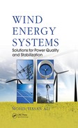
The second design strategy is to produce flywheels with a lightweight rotor turning at very high rotational velocities (up to 100,000 rpm). This approach results in compact, lightweight energy storage devices. Modular designs are possible, with a large number of small flywheels possible as an alternative to a few large flywheels. However, rotational losses due to drag from air and bearing losses result in significant self-discharge, which poses problems for long-term energy storage. High-velocity flywheels are therefore operated in vacuum vessels to eliminate air resistance. The use of magnetic bearings helps improve the problems with bearing losses. Several projects are developing superconducting magnetic bearings for high-velocity flywheels. The near elimination of rotational losses will provide flywheels with high charge and discharge efficiency. The peak power transfer ratings depend on the power ratings in the power electronic converter and the electric machine. Flywheel applications under consideration include automobiles, buses, high-speed rail locomotives, and energy storage for electromagnetic catapults on next-generation aircraft carriers. The high rotational velocity also results in the need for some form of containment vessel around the flywheel in case the rotor fails mechanically. The added weight of the containment can be especially important in mobile applications. However, some form of containment is necessary for stationary systems as well. The largest commercially available flywheel system is about 5 MJ/1.6 MVA weighing approximately 10,000 kg. Flywheel energy storage can be implemented in several power system applications. If an FES system is included with a FACTS or custom power device with a DC bus, an inverter is added to couple the flywheel motor or generator to the DC bus. For example, a flywheel based on an AC machine could have an inverter interface to the DC bus of the custom power device, as shown in Figure 7.4. Flywheel energy storage has been considered for several power system applications, including power quality applications as well as peak shaving and stability enhancement.
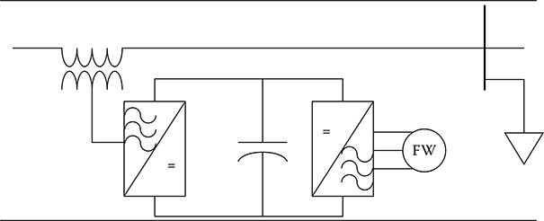
Figure 7.4 Flywheel energy storage coupled to a dynamic voltage.
7.2.5 Pumped Hydroelectric Energy Storage
Hydroelectric storage is a process that converts electrical energy to potential energy by pumping water to a higher elevation, where it can be stored indefinitely and then released to pass through hydraulic turbines and generate electrical energy. A typical pumped-storage development is composed of two reservoirs of equal volume situated to maximize the difference in their levels. These reservoirs are connected by a system of waterways along which a pumping generating station is located. Under favorable geological conditions, the station will be located underground; otherwise, it will be situated on the lower reservoir. The principal equipment of the station is the pumping-generating unit, which is generally reversible and used for both pumping and generating, functioning as a motor and pump in one direction of rotation and as a turbine and generator in opposite rotation.
7.2.6 Flow Batteries
Flow batteries (FBs) are a promising technology that decouples the total stored energy from the rated power. The rated power depends on the reactor size, whereas the stored capacity depends on the auxiliary tank volume. These characteristics make the FB suitable for providing large amounts of power and energy required by electrical utilities. FBs work in a similar way as hydrogen fuel cells (FCs), as they consume two electrolytes that are stored in different tanks (no self-discharge), and there is a microporous membrane that separates both electrolytes but allows selected ions to cross through, creating an electrical current. There are many potential electro-chemical reactions, usually called reduction–oxidation reaction (REDOX), but only a few of them seem to be useful in practice [45].
Figure 7.5 shows a schematic of an FB. The power rating is defined by the flow reactants and the area of the membranes, whereas the electrolyte tank capacity defines the total stored energy. In a classical battery the electrolyte is stored in the cell itself, so there is a strong coupling between the power and energy rating. In the cell (flow reactor), a reversible electrochemical reaction takes place, producing (or consuming) electric DC current. At this time, several large- and small-scale demonstration and commercial products use FB technology.
The main advantages of FB technology are (1) high power and energy capacity; (2) fast recharge by replacing exhaust electrolyte; (3) long life enabled by easy electrolyte replacement; (4) full discharge capability; (5) use of nontoxic materials; and (6) low-temperature operation. The main disadvantage of the system is the need for moving mechanical parts such as pumping systems that make system miniaturization difficult. Therefore, the commercial uptake to date has been limited.
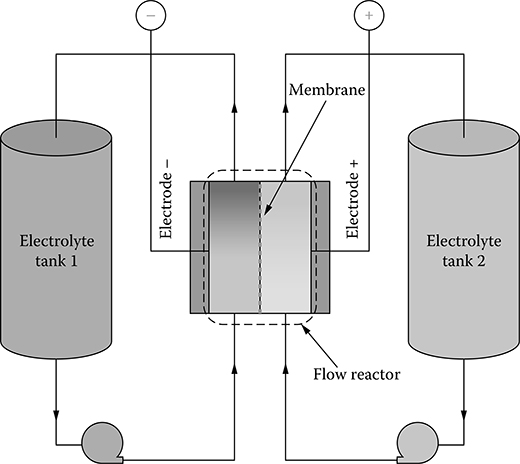
Figure 7.5 (See color insert.) Flow battery cell.
7.2.7 Compressed Air Energy Storage
Compressed air energy storage (CAES) is a technology that stores energy as compressed air for later use. Energy is extracted using a standard gas turbine, where the air compression stage of the turbine is replaced by the CAES, thus eliminating the use of natural gas fuel for air compression. System design is complicated by the fact that air compression and expansion are exothermic and endothermic processes, respectively. With this in mind, three types of systems are considered to manage the heat exchange:
Isothermal storage, which compresses the air slowly, thus allowing the temperature to equalize with the surroundings. Such a system works well for small systems where power density is not paramount.
Adiabatic systems, which store the released heat during compression and feed it back into the system during air release. Such a system needs a heat-storing device, complicating the system design.
Diabatic storage systems, which use external power sources to heat or cool the air to maintain a constant system temperature. Most commercially implemented systems are of this kind due to high power density and great system flexibility, albeit at the expense of cost and efficiency.
CAES systems have been considered for numerous applications, most notably for electric grid support for load leveling applications. In such systems, energy is stored during periods of low demand and then converted back to electricity when the electricity demand is high. Commercial systems use natural caverns as air reservoirs to store large amounts of energy; installed commercial system capacity ranges from 35 to 300 MW.
7.2.8 Thermoelectric Energy Storage
Thermoelectric energy storage (TEES) for solar thermal power plants consists of a synthetic oil or molten salt that stores energy in the form of heat collected by solar thermal power plants to enable smooth power output during daytime cloudy periods and to extend power production for 1–10 h after sunset. End-use TEES stores electricity from off-peak periods through the use of hot or cold storage in underground aquifers, water or ice tanks, or other storage materials and uses this stored energy to reduce the electricity consumption of building heating or air conditioning systems during times of peak demand.
7.2.9 Hybrid Energy Storage Systems
Certain applications require a combination of energy, power density, cost, and life cycle specifications that cannot be met by a single energy storage device. To implement such applications, hybrid energy storage devices (HESDs) have been proposed. HESDs electronically combine the power output of two or more devices with complementary characteristics. HESDs all share a common trait: combining high-power devices (devices with quick response) and high-energy devices (devices with slow response). Proposed HESDs are listed next, with the energy-supplying device listed first followed by the power-supplying device:
Battery and electric double-layer capacitor (EDLC)
FC and battery or EDLC
CAES and battery or EDLC
Battery and flywheel
Battery and SMES
7.3 Energy Storage Systems Compared
There are relative advantages and disadvantages of the various energy storage systems. For example, some of the disadvantages of BESSs include limited life cycle, voltage and current limitations, and potential environmental hazards. Again, some of the disadvantages of pumped hydroelectric are large unit sizes and topographic and environmental limitations. The major problems of confronting the implementation of SMES units are the high cost and environmental issues associated with strong magnetic field. Relatively short duration, high frictional loss (windage), and low-energy density restrain the flywheel systems from the application in energy management. Similar to flywheels, the major problems associated with capacitors are the short durations and high-energy dissipations due to self-discharge loss. However, among all energy storage systems, SMES is the most effective from the viewpoints of fast response, charge and discharge cycles, and control ability of both active and reactive powers simultaneously.
7.4 Using SMES to Minimize Fluctuations in Power, Frequency, and Voltage of Wind Generator Systems
Recent developments and advances in both superconducting and power electronics technology have provided the power transmission and distribution industry with SMES systems. SMES is a large superconducting coil capable of storing electric energy in the magnetic field generated by DC current flowing through it. The real power as well as the reactive power can be absorbed (charging) by or released (discharging) from the SMES coil according to system power requirements. Since the successful commissioning test of the Bonneville Power Administration (BPA) 30 MJ unit, SMES systems have received much attention in power system applications, such as diurnal load demand leveling, frequency control, automatic generation control, and uninterruptible power supplies. A gate turn-off (GTO) thyristor-based SMES unit is able to absorb and inject active as well as reactive powers simultaneously in rapid response to power system requirements. Therefore, it can act as a good tool to decrease voltage and frequency fluctuations of the system considerably. With this view, minimization of fluctuations of line power and terminal voltage of wind generators by the SMES is considered in this book.
The model system as shown in Figure 7.6 was used for the simulation [2]. The power system model belongs to Ulleung Island in South Korea. The model system consists of two diesel generators (4.5 MVA and 1.5 MVA), two hydroelectric generators (0.6 MVA and 0.1 MVA), one wind turbine generator (0.6 MVA IG), and a load of 6 MW. In this work, to evaluate the performance of SMES systems in detail, another load of 2 MW is also considered. When a 2 MW load is considered, ratings of some of the generators and transformers are changed, as shown in red colors in Figure 7.6. A condenser C is connected to the terminal of the wind generator to compensate the reactive power demand for the induction generator at steady-state. The value of C has been chosen so that the power factor of the wind power station becomes unity when it is generating the rated power (P = 0.6, V = 1.0). The SMES unit is located at the induction generator terminal bus. The automatic voltage regulator (AVR) control system models for the diesel and hydraulic generators and the governor (GOV) control system model for the hydroelectric generator used in this work are the built-in models of Power System Computer Aided Design (PSCAD)/ Electromagnetic Transients in DC (EMTDC). However, the GOV control system model for the diesel generator used in this work is shown in Figure 7.7. The typical values for the parameters of the diesel governor model are shown in Table 7.1, whereas synchronous generator parameters as well as induction generator parameters used for this simulation are shown in Table 7.2.
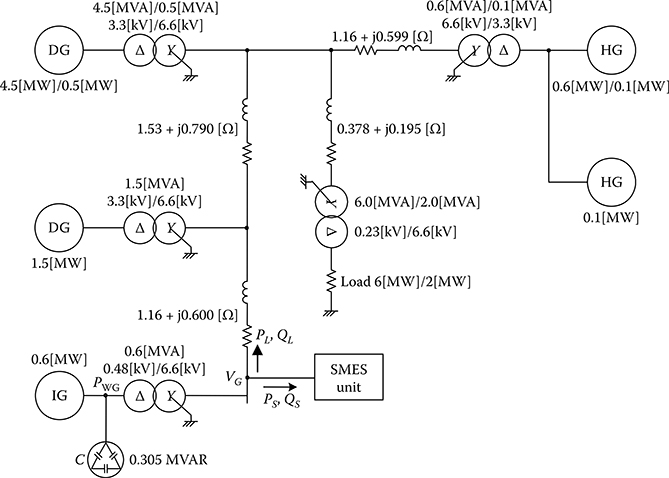
Figure 7.6 (See color insert.) Power system model.

Figure 7.7 Diesel–governor model.
Table 7.1 Diesel Governor Parameters

Table 7.2 Generator Parameters

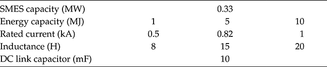
The SMES unit model used in this work is shown in Figure 7.8. It consists of a WYE-Delta (6.6 kV/1.2 kV) transformer, a six-pulse pulse width modulation (PWM) voltage source converter using an insulated gate bipolar transistor (IGBT), a DC link capacitor, a two-quadrant DC-to-DC chopper using IGBT, and an inductance as a superconducting coil. The VSC and the DC-to-DC chopper are linked by a DC link capacitor. In this work, to evaluate in detail the performance of the SMES system to minimize frequency fluctuations, different energy capacities of the SMES are considered. The parameters for the proposed SMES are shown in Table 7.3.
The PWM VSC provides a power electronic interface between the AC power system and the superconducting coil. The DC link voltage EDC and grid point voltage VG are maintained as constant by the VSC. In this model system, the transformer connecting the VSC and the AC system is expressed by an RL circuit. Since a leakage reactance of a transformer is, in general, much greater than the winding resistance, the active and reactive powers of the SMES system are proportional to the d- and q-axis currents and thus also to the d- and q-axis voltages as expressed by (7.8). Based on this concept, the control system of the VSC is constructed.

Figure 7.8 Configuration of SMES unit.
Table 7.3 SMES Parameters
The control system of the VSC is shown in Figure 7.9. The proportional-integral (PI) controllers determine reference d- and q-axis currents by using the difference between the DC link voltage EDC and reference value EDC-ref, and the difference between terminal voltage VG and reference value VG-ref, respectively. The reference signal for the VSC is determined by converting d- and q-axis voltages obtained from the difference between the reference d–q-axes currents and their detected values. Parameters of the Proportional-Integral (PI) controllers are determined by trial and error method. The PWM signal is generated for IGBT switching by comparing the reference signal, which is converted to a three-phase sinusoidal wave with the triangular carrier signal.
The superconducting coil is charged or discharged by adjusting the average voltage, Vsm-av, across the coil, which is determined by the duty cycle of the two-quadrant DC-to-DC chopper. Based on this concept, the control system of a two-quadrant DC-to-DC chopper is constructed as shown in Figure 7.10. The duty cycle is determined by the PI controller. For example, when the duty cycle is larger than 0.5 or less than 0.5, the stored energy of the coil is either charging or discharging. To generate the PWM gate signals for the IGBT of the chopper, the reference signal is compared with the triangular signal.
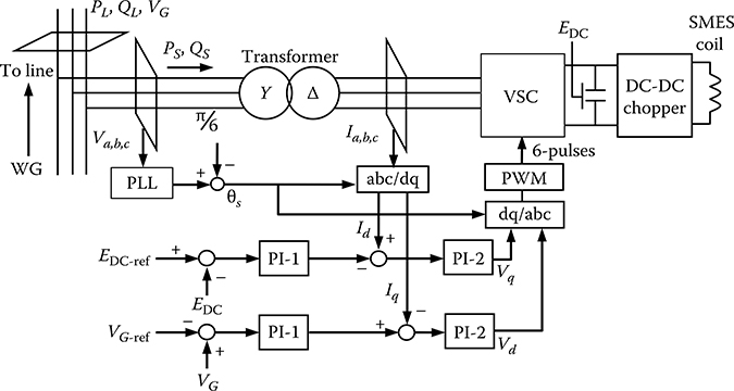
Figure 7.9 Control system of the VSC.

Figure 7.10 Control system of two-quadrant DC-DC chopper.

Figure 7.11 Determination of reference value.
The reference value of the transmission line power PG-ref is determined by a low-pass filter (LPF) as shown in Figure 7.11. LPF consists of a first-order delay system. Though it is very simple, a reference value with enough smoothing effect can be obtained by this type of LPF.
7.4.1 Method of Calculating Power System Frequency
In this study, the index of the smoothing effect is used in power system frequency analysis. Power system frequency fluctuation occurs due to an imbalance between supply and load power in power system. Then, the frequency fluctuation can be described using two components: the rate of generator output variation, KG (MW/Hz), and load variation, KL (MW/ Hz). They are representing the amount of power variation causing 1 Hz frequency fluctuation. When generator output variation, ΔG (MW), and load variation, ΔL (MW), occur, frequency fluctuation of the power system, ΔF (Hz), is expressed as
where K is frequency characteristic constant. In general, frequency characteristic is expressed as percentage KG (expressed as %KG) for the total capacity of all generators and percentage KL (expressed as %KL) for the total load. In general, it is known that %KG and %KL are almost constant and generally take a value of 8–15% MW/Hz and 2–6% MW/Hz, respectively. However, KL and KG change greatly during a day because the number of parallel generators changes depending on the amount of load during a day. And when power imbalance ΔP occurs in power system, frequency fluctuation ΔP/K cannot occur immediately due to the governor characteristic and generator inertia. Normally, ΔF converges to a new steady-state value in 2 to 3 sec. In general, when ΔP is changing slowly, the relationship between ΔP and ΔF can be expressed as follows:
where ΔP = ΔG – ΔL. Since changing load is not considered in this study, ΔL is 0. Time constant, T (sec), depending on the setting of generator governor and generator inertia, is generally 3 to 5 sec. In this study, power system capacity is assumed to be 100 MW, and frequency characteristic K (MW/Hz) is selected to 8 MW/Hz. This selection means that adjustability of the system frequency is weak, resulting in a severe situation. Similarly, time constant T is selected to 3 sec. In this study, frequency fluctuation in the power system is evaluated using Equation (7.11). Therefore, frequency fluctuation, ΔF, is obtained as shown in Figure 7.12.

Figure 7.12 Frequency calculation model.

Figure 7.13 Wind speed data.
Table 7.4 Specifications of Wind Speed
Average [m/s] |
10.1 |
Minimum [m/s] |
7.3 |
Maximum [m/s] |
11.3 |
Standard deviation [m/s] |
0.79 |
7.4.2 Simulation Results and Discussions
To evaluate the performance of the SMES strategy to minimize system frequency fluctuations, simulations are carried out considering variable wind speed data as shown in Figure 7.13. The specifications of wind speed are given in Table 7.4. The simulation time and time step were chosen as 60 sec and 10 msec, respectively. Figures 7.14 and 7.15 show the responses of active powers of the wind generators, diesel generators and hydraulic generators, and the system frequency without SMES systems with 2 MW and 6 MW loads, respectively. It is seen that without the wind generator the system frequency is maintained at the nominal value of 60 Hz; however, when the wind generator is used in the power system model the system frequency considerably fluctuates, especially for low load (2 MW load). This fact motivates the use of the SMES method to minimize system frequency and power fluctuations resulting from the wind generator system.
7.4.2.1 Effectiveness of SMES Systems on Minimizing Wind Generator Power, Frequency, and Voltage Fluctuations
Figures 7.16 and 7.17 show the responses of active powers of the wind generator, diesel generators and hydraulic generators, the transmission line power, and the system frequency using 10 MJ SMES with 2 MW and 6 MW loads, respectively. It is seen that because of the use of the SMES, the system frequency fluctuations are minimized well, and the frequency is maintained almost at the level of the nominal value of 60 Hz for both loads. Also, it is observed that the SMES system can successfully smooth the transmission line power for both loads. Thus, the smoothed power can be supplied to the consumers. Although the grid voltage responses are not shown here, it is seen that the SMES system can minimize the oscillations of grid voltage. As a whole, the SMES system can be considered a very effective tool to minimize frequency, power, and voltage fluctuations of power systems including wind generators.
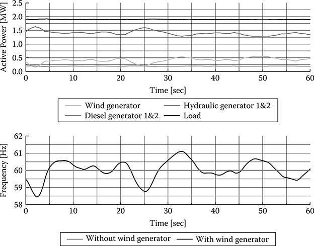
Figure 7.14 (See color insert.) Responses of active power and system frequency without SMES (Load 2 MW).
7.4.2.2 Comparison among Energy Capacities of SMES Systems to Minimize Wind Generator Power, Frequency, and Voltage Fluctuations
In this work, to evaluate in detail the performance of SMES systems to minimize frequency, power, and voltage fluctuations, extensive simulations were carried out considering different energy capacities of SMES. Figure 7.18 shows the responses of active power of a wind generator, transmission line power, and system frequency using 10 MJ, 5MJ, and 1 MJ SMES with a 2 MW load. It is seen that the performance of the 10 MJ SMES is the best from the viewpoint of minimization of fluctuations of system frequency and line power. The 5 MJ SMES can minimize the power and frequency fluctuations well; however, the 1 MJ SMES has little ability to minimize frequency and power fluctuations. In general, the larger the capacity of SMES is, the better the ability of fluctuations minimization becomes. However, if the large size of SMES is adopted, its cost increases, making the installation of SMES impractical. From this viewpoint, the 5 MJ SMES is a trade-off between higher cost and better performance. Therefore, the SMES capacity for fluctuations minimization of power, frequency, and voltage should be selected considering the viewpoint of cost-effectiveness.

Figure 7.15 (See color insert.) Responses of active power and system frequency without SMES (Load 6 MW).

Figure 7.16 (See color insert.) Responses of active power and system frequency with 10 MJ SMES (Load 2 MW).

Figure 7.17 (See color insert.) Responses of active power and system frequency with 10 MJ SMES (Load 6 MW).
Figures 7.19, 7.20, and 7.21 show the responses of real power, storage energy, coil current, coil voltage, DC link current, and DC link voltage with 2 MW and 6 MW loads corresponding to 5 MJ, 10 MJ, and 1 MJ SMES systems, respectively. In all cases it is seen that the SMES is being charged and discharged according to system power requirements to minimize frequency fluctuations. The SMES energy and coil current are well within the ranges of their rated values. Moreover, the PWM voltage source converter can maintain the DC link voltage constant.

Figure 7.18 (See color insert.) Responses of active power and system frequency with different capacities of SMES (Load 2 MW).
7.4.3 SMES Power and Energy Ratings
It is important to know the optimal power and energy ratings of SMES systems so that their cost is minimal. In this work, the relationship between SMES power capacity and the smoothing ability is investigated by evaluating a wind turbine generator output, PWG, and reference value of transmission line power, PG-ref, with the condition that the LPF time constant is changed from 3 to 300 sec. Since a large number of wind turbine generators are going to be connected to a power system in the near future, a percentage of wind turbine generators to the total power system capacity is assumed fairly large: 10% (10 MW) and 20% (20 MW) in this study. Smoothing of the wind turbine generator output is investigated by using PG-ref instead of an SMES unit in the calculation to estimate a required capacity of the SMES [3].

Figure 7.19 Responses of 5 MJ SMES.
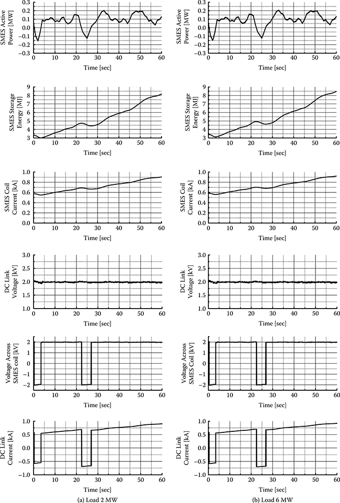
Figure 7.20 Responses of 10 MJ SMES.

Figure 7.21 Responses of 11 MJ SMES.
The model system used in this simulation analysis is shown in Figure 7.22. Table 7.5 shows the parameters for the induction generator shown in Figure 7.22. The wind speed patterns and conditions used in the simulation are shown in Figure 7.23 and Table 7.6. Three kinds of wind speed patterns with relatively large fluctuations are selected. SMES output is assumed to be the difference between PWG and PG-ref in this simulation, and then a standard deviation of the SMES output, σ, is calculated. In addition, smoothing effect is evaluated by using frequency fluctuation ΔF (ΔFWG, ΔFG-ref). ΔF is calculated by applying PWG and PG-ref to the frequency calculation model. The required SMES power capacity for smoothing PWG and an LPF time constant suitable for the reference value with enough smoothing effect are investigated by using σ and ΔF in this simulation.

Figure 7.22 Model system.
Table 7.5 Induction Generator Parameters

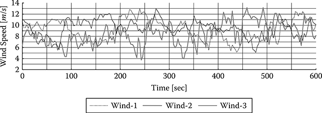
Figure 7.23 (See color insert.) Wind speed.
Table 7.6 Wind Speed Condition
Wind Data’s Name |
Average Wind Speed [m/s] |
Standard Deviation of Wind Speed [m/s] |
||
Wind-1 |
Medium |
9.28 |
Large |
1.82 |
Wind-2 |
Medium |
8.45 |
Large |
2.01 |
Wind-3 |
Medium |
9.44 |
Medium |
1.54 |
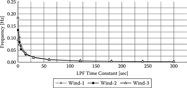
Figure 7.24 (See color insert.) Maximum frequency fluctuation (WG capacity 10%). 0.0

Figure 7.25 (See color insert.) Maximum frequency fluctuation (WG capacity 20%).
Figures 7.24 and 7.25 show the maximum frequency fluctuation with respect to the LPF time constant for two cases of wind generator capacity, 10% and 20%, respectively. Frequency fluctuation decreases as the LPF time constant increases. Therefore, if the transmission line power is compensated according to reference value PG-ref, it is possible to decrease the system frequency fluctuation due to the wind generator output fluctuations. It is clear from Figures 7.24 and 7.25 that the maximum frequency fluctuations converge to almost 0 Hz when the LPF time constant is over 120 sec.
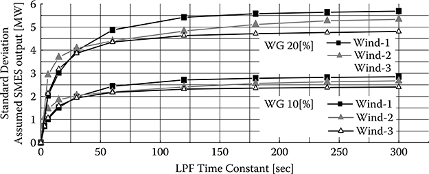
Figure 7.26 (See color insert.) Assumed SMES output standard deviation.
Figure 7.26 shows the standard deviation, σ, of the SMES output with respect to the LPF time constant for the two wind generator capacities (10% and 20%). σ increases as the LPF time constant increases. However, as can be seen from Figure 7.26, the function of σ is not monotonous and saturates where the LPF time constant is about 120 sec. Therefore, if a longer LPF time constant and thus the larger capacity of SMES are adopted, the frequency deviation becomes small; however, the degree of improvement also becomes small. Table 7.7 shows σ and ΔF in each condition. Considering these results, the reference value of transmission line power corresponding to σ for 120 sec, the LPF time constant may be sufficient for the smoothing control. Consequently, it can be said that if a 120 sec LPF time constant is adopted, the suitable reference value with enough smoothing effect can be obtained. If the power capacity of the SMES is determined based on the value of 2σ, approximately 95% of necessary smoothing output can be achieved according to the characteristic of standard deviation. This capacity of SMES is applied for compensating PWG fluctuations in the next simulation analysis.
Required energy storage capacity of the SMES is estimated when the latter compensates for the wind generator’s fluctuating power according to reference power PG-ref calculated using the LPF with several time constants including the best one determined in the previous section. Figure 7.27 shows the model for this evaluation. The wind power output is assumed as an ideal periodic sinusoidal wave form or trapezoidal wave form, and then the behavior of the SMES stored energy is investigated. To evaluate the influence of the period of wind power fluctuation on the smoothing effect, five LPF time constants (30, 60, 120, 180, and 300 sec) are used and the period of wind power fluctuation is varied from 10 to 1,200 sec. The required energy capacity of SMES can be determined as a difference of the maximum and the minimum values of the stored energy.

Figure 7.27 Simulation model.
Table 7.7 The Standard Deviation of SMES Output and Maximum Frequency Fluctuation in Each Condition
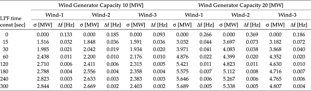
Table 7.8 shows a difference of the maximum and the minimum values of the SMES stored energy with respect to the period of fluctuation for several LPF time constants in two cases. In Table 7.8, the result in the case of an extremely long period (12,000 sec) is also indicated. From these results, (7.12) can be established. Consequently, the required SMES energy storage capacity to compensate fluctuating wind power with relatively long periodic change can be decided approximately by using (7.12), and the energy storage capacity greater than this is not needed [3–4].
where E (MJ) is the saturated value of the range of energy change of the SMES, T (sec) is the LPF time constant, and PWF (MW) is the rated wind farm output.
Since it is shown that the frequency fluctuation can be decreased sufficiently by the reference value PG-ref, which is determined based on a LPF time constant of 120 sec, this value is used to calculate the reference value using the system shown in Figure 7.11. The model system used in the simulation analysis is shown in Figure 7.28. In this simulation analysis, the power capacity of the SMES is determined based on the value of 2σ, because the necessary smoothing effect can be achieved by an SMES with this capacity as shown in the previous section. When the power capacity of the wind generator is 10% of the entire power system, then the SMES power capacity is 5.5 MW (2σ = 2.7 × 2 = 5.4, where σ = 2.7 MW). Similarly, when the wind generator capacity is 20%, the SMES capacity is 11 MW (σ = 5.4 MW). SMES power capacities in these two cases are both 55% of the wind generator rated capacities (10 and 20% of the entire power system). In the following simulations, two cases using SMES systems with capacities of 55 and 50% of the wind generator rated capacity are examined for the three wind speed patterns.
Table 7.8 The Range of Changing SMES Energy for Each Input

Figure 7.29 shows responses of wind generator output and transmission line power when the capacity of the wind generator is 10% of the entire power system and the SMES power capacity is 55% and 50% of the wind generator. Figure 7.30 shows responses of frequency fluctuation under the same condition as Figure 7.29. Figure 7.31 shows responses of wind generator output and transmission line power when the capacity of the wind generator is 20% and the SMES power capacity is 55% and 50%. Figure 7.32 shows responses of frequency fluctuation under the same condition as Figure 7.30. Table 7.9 shows values of the maximum frequency fluctuation in each case. As shown in Figures 7.29 to 7.32, since necessary compensating power exceeds the capacity of the SMES system in some instances, large frequency fluctuation occurs, especially in the case of wind-2. It can be seen in Table 7.9 that frequency fluctuations in SMES power capacity at 50% are greater than those in SMES power capacity at 55%. The maximum frequency fluctuation in SMES power capacity at 50% is 0.061 Hz for 10% WG and 0.122 Hz for 20% WG, whereas the maximum frequency fluctuation in SMES power capacity at 55% is 0.006 Hz for 10% WG and 0.012 Hz for 20% WG. The former is approximately 10 times larger than the latter. Therefore, it can be said that the SMES with 50% power capacity of that of wind generator is not sufficient.
Consequently, it can be concluded that if an LPF time constant of 120 sec is selected and an SMES system with 55% power capacity of that of wind generator is adopted, a suitable reference value for the transmission line power can be obtained and then sufficient smoothing effect can be achieved. Moreover, the energy storage capacity of the SMES can be determined to 2,400 MJ according to (7.12).

Figure 7.28 Model system.

Figure 7.29 (See color insert.) Wind generator output and transmission line power (WG capacity 10%).
7.5 Power Quality Improvement Using a Flywheel Energy Storage System
A flywheel energy storage system using a squirrel-cage induction machine is explained in this context. The system uses the squirrel-cage induction machine, which is widely available and inexpensive, and the simple volt/hertz control technique with just nameplate data as machine parameters. Therefore, no complex parameter measurement is necessary, and the system has an advantage on parallel operation because adding or replacing units is straightforward. Hence, it can easily operate with different types of storage or distributed energy sources in DC bus microgrid systems. Moreover, the control scheme improves the overall stability of the DC bus system [66].

Figure 7.30 (See color insert.) Frequency fluctuation (WG capacity 10%).

Figure 7.31 (See color insert.) Wind generator output and transmission line power (WG capacity 20%).
Advances in power electronics, magnetic bearings, and flywheel materials have made flywheel systems a viable energy storage option. Although it has higher initial cost than batteries, flywheel energy storage has advantages such as longer lifetime, lower operation and maintenance costs, and higher power density (typically by a factor of 5 to 10). Flywheel systems have been used in many applications instead of or in conjunction with batteries. Machines such as permanent magnet (PM) machines, synchronous reluctance machines, synchronous homopolar machines, and induction machines have been explored for flywheel motors and generators. PM machines have advantages such as lower rotor losses, high power factor, efficiency, and power density. However, high-power magnets are costly and have an inherent disadvantage of spinning losses.

Figure 7.32 (See color insert.) Frequency fluctuation (WG capacity 20%).
Synchronous homopolar machines, although they have been researched for various applications, are not widely used in practice. Synchronous reluctance machines can be a viable choice for a flywheel motor or generator, but the machines are not easily available. Induction machine-based flywheel systems have been investigated, and it has been suggested that the rugged and inexpensive induction machines are good candidates for high-power flywheel motors or generators. Field-oriented vector controllers are generally used for faster dynamic response, which require complex machine parameter measurements and complicated controllers.
Table 7.9 Maximum Frequency Fluctuation in Each Condition

However, the majority of the fast disturbances are shorter than several seconds, and storage devices needed to store the intermittent generation of renewable energy sources do not necessarily have to be fast if they are not focusing on transient performance improvement. Considering the overall cost, it would be more efficient for a microgrid system to use a combination of faster storage devices for short transient and slower but inexpensive storage units for massive energy charge and discharge with renewable energy sources such as wind turbines and photovoltaic systems.
7.5.1 DC Bus Microgrid System
Among the microgrids that have been researched recently, low-voltage DC (LVDC) bus-based systems have received attention because of advantages such as fast control without need for communication, a variety of DC energy sources and loads, and efficiencies on system size and cost. A block diagram of a typical DC bus microgrid system is shown in Figure 7.33.
The LVDC systems use the voltage droop technique, involving the DC bus voltage as a command signal. DC bus systems do not have the functional issues of AC systems such as synchronization and reactive power compensation. Unlike large-scale distribution systems, the LVDC microgrid system does not have a resistive loss issue because the length of the bus is much shorter. Also, sharing a DC bus has a structural advantage because all the energy sources and loads are connected via DC-to-DC or DC-to-AC voltage source converters that use DC voltage as their medium. Another layer of DC-to-AC converters is necessary for some subsystems to make an AC bus system.

Figure 7.33 Conceptual diagram of a DC bus microgrid system.
Using the fast-acting power electronics converters, constant voltage can be supplied to the loads regardless of some fluctuations on the bus side, and the renewable energy sources can readily generate maximum power with maximum power point tracking (MPPT) techniques. As a small-scale power system, a microgrid can have relatively higher load fluctuations, especially when it is not operating in grid-connected mode. This is because the inertia of the generators is not as large as that found in the large-scale synchronous generators. Generation of power from the renewable energy sources relies heavily on natural conditions, and they are intermittent. Hence, energy storage devices are required for stable operation of a microgrid system in either grid-connected or islanded operations. A flywheel-based energy storage system is investigated in this work.
To develop a cost-effective system, a squirrel-cage induction machine is selected for the motor or generator of the flywheel energy storage in this work. A per-phase equivalent circuit of an induction machine is shown in Figure 7.34. Easy parallel operation is an important factor in energy storage for higher capacity.
7.5.2 Volt/Hertz Control
Volt/hertz control has been widely used for induction machine speed control. The field-oriented vector control technique has been used for applications that need fast response, but it requires parameter measurements, current feedback, a machine model, and controller tuning. On the DC bus Flywheel contrary, all of the information necessary to run an induction machine in rated condition, such as voltage, speed, and slip, can be found on the nameplate of the machine for volt/hertz control.
Much research on flywheel energy storage systems has used field-oriented controllers because the applications need quite fast energy flow, for example, Uninterruptable Power Supply (UPS) application compensating the voltage dip. However, if an energy storage system absorbs or releases the energy in slow dynamics, volt/hertz control can be a valid candidate due to its simplicity and inherent stability.
7.5.3 Microgrid System Operation
The microgrid system shown in Figure 7.33 uses the DC bus voltage as a control signal. Hence, a prime mover, such as a grid-connected converter or micro turbine unit, does not control the voltage tightly at a fixed reference voltage to reflect the energy flow on the bus voltage if it is in the nominal operating region above the minimum threshold. All of the renewable energy source units are operating in the power mode, which is generating its maximum power when the energy is available. Hence, the bus voltage will rise above the nominal operating range if the generation is larger than the load power consumption. The storage devices detect the excessive energy in the bus and absorb it. If the generated energy is large enough to exceed the maximum threshold, the grid-connected converter can push it back to the grid.
When the DC bus voltage gets lower than the discharge threshold due to the increased load or decreased generation, the energy stored in the storage units is discharged to the bus to maintain the bus voltage at the minimum level. If all the energy storages and generators are not able to hold the bus voltage at the minimum level, load shedding can be initiated by disconnecting some of the power electronics converters supporting lower priority loads. If different kinds of storage or load control units are connected to the bus, the priority can be easily controlled by setting the thresholds differently. The units in the microgrid are autonomously operating using the bus voltage without communicating between units or to a central controller; hence, addition, replacement, or removal of the units can be done easily without any major change in the control configuration unlike the centrally controlled system.
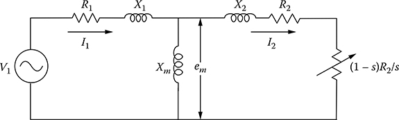
Figure 7.34 Induction machine per-phase equivalent circuit.
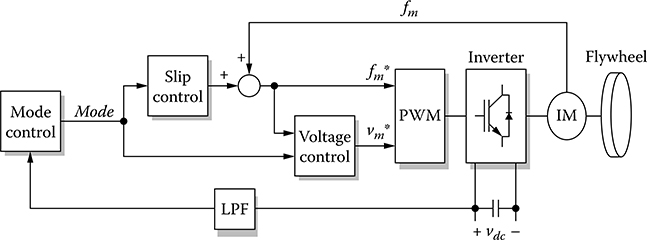
Figure 7.35 Block diagram of flywheel drive system.
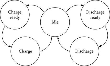
Figure 7.36 Controller state machine.
7.5.4 Control of Flywheel Energy Storage System
The control block diagram of the flywheel drive system is shown in Figure 7.35. The controller consists of three parts—mode control, slip control, and voltage control—to generate the proper voltage and frequency for the flywheel induction motor or generator. The low-pass filter filters out the high-frequency voltage fluctuations. The mode control determines the operating mode based on the bus voltage. The operating modes of the proposed flywheel energy storage system, and the state machine of the mode control can be seen in Figure 7.36. Each mode has associated voltage levels predefined in the mode control, as shown in Figure 7.37.
7.5.5 Stability Consideration
It is well known that DC power distribution systems can have stability issues due to the negative impedance of the connected converters, even if the individual subsystems are stable. The input impedance of the converter can be expressed as (7.13). The input impedance of the converters becomes negative when they are operating in constant power mode. where Δ denotes the deviation from the steady-state operating point values.

Figure 7.37 Bus voltage thresholds for control.
The power electronics converters can tightly control their output power as almost constant, and the negative impedance affects the DC bus stability adversely. It has also been suggested that the output impedances of the sources Zo should be smaller than input impedances of the loads Zi for the overall stability of the DC bus.
Although this is not a direct issue for the proposed energy storage system because it does not operate in constant power mode, its effect on overall system stability needs to be considered. The proposed system controls the power with the slip and constant volt/hertz ratio, which keeps the torque proportional to the slip. When the flywheel energy storage system charges the energy from the bus, the slip is proportional to the bus voltage. Hence, the power that the storage system takes from the bus is proportional to the bus voltage and the impedance of the system is always positive. On the other hand, the slip is inversely proportional to the change of the bus voltage, which lowers the overall source impedance because the DC current the storage system discharges increases as the bus voltage decreases. Therefore, the energy storage system can improve the overall stability of the system in either operating mode.

Figure 7.38 Configuration of a DFIG wind turbine equipped with a supercapacitor ESS connected to a power grid.
7.6 Constant Power Control of DFIG Wind Turbines with Supercapacitor Energy Storage
This section discusses a novel two-layer constant power control (CPC) scheme for a wind farm equipped with DFIG wind turbines, where each WTG is equipped with a supercapacitor energy storage system (ESS). The CPC consists of a high-layer wind farm supervisory controller (WFSC) and low-layer WTG controllers. The high-layer WFSC generates the active power references for the low-layer WTG controllers of each DFIG wind turbine according to the active power demand from the grid operator. The low-layer WTG controllers then regulate each DFIG wind turbine to generate the desired amount of active power, where the deviations between the available wind energy input and desired active power output are compensated by the ESS [67].
Figure 7.38 shows the basic configuration of a DFIG wind turbine equipped with a supercapacitor-based ESS. The low-speed wind turbine drives a high-speed DFIG through a gearbox. The DFIG is a wound-rotor induction machine. It is connected to the power grid at both stator and rotor terminals. The stator is directly connected to the grid, whereas the rotor is fed through a variable-frequency converter, which consists of a rotor-side converter (RSC) and a grid-side converter (GSC) connected back to back through a DC link and usually with a rating of a fraction (25–30%) of the DFIG nominal power. As a consequence, the WTG can operate with the rotational speed in a range of ±25–30% around the synchronous speed, and its active and reactive powers can be controlled independently. In this work, an ESS consisting of a supercapacitor bank and a two-quadrant DC-to-DC converter is connected to the DC link of the DFIG converters. The ESS serves as either a source or a sink of active power and therefore contributes to control the generated active power of the WTG. The value of the capacitance of the supercapacitor bank can be determined by
where Cess is in farads, Pn is the rated power of the DFIG (watts), VSC is the rated voltage of the supercapacitor bank (volts), and T is the desired time period (seconds) that the ESS can supply or store energy at the rated power (Pn) of the DFIG.
The use of an ESS in each WTG rather than a large single central ESS for the entire wind farm is based on two reasons. First, this arrangement has a high reliability because the failure of a single ESS unit does not affect the ESS units in other WTGs. Second, the use of an ESS in each WTG can reinforce the DC bus of the DFIG converters during transients, thereby enhancing the low-voltage ride-through capability of the WTG.
7.6.1 Control of Individual DFIG Wind Turbines
The control system of individual DFIG wind turbines generally consists of two parts: (1) the electrical control of the DFIG; and (2) the mechanical control of the wind turbine blade pitch angle and yaw system. Control of the DFIG is achieved by controlling the RSC, the GSC, and the ESS as shown in Figure 7.38. The control objective of the RSC is to regulate the stator-side active power Ps and reactive power Qs independently. The control objective of the GSC is to maintain the DC link voltage Vdc constant and to regulate the reactive power Qg that the GSC exchanges with the grid. The control objective of the ESS is to regulate the active power Pg that the GSC exchanges with the grid.
7.6.2 Control of the RSC
Figure 7.39 shows the overall vector control scheme of the RSC, in which the independent control of the stator active power Ps and reactive power Qs is achieved by means of rotor current regulation in a stator-flux-oriented synchronously rotating reference frame. Therefore, the overall RSC control scheme consists of two cascaded control loops. The outer control loop regulates the stator active and reactive powers independently, which generates the reference signals i*dg and i*dg of the d- and q-axis current components, respectively, for the inner-loop current regulation. The outputs of the two current controllers are compensated by the corresponding cross-coupling terms vdg0 and vdg0, respectively, to form the total voltage signals vdg and vqg. They are then used by the PWM module to generate the gate control signals to drive the RSC. The reference signals of the outer-loop power controllers are generated by the high-layer WFSC.

Figure 7.39 Overall vector control scheme of the RSC.
7.6.3 Control of the GSC
Figure 7.40 shows the overall vector control scheme of the GSC, in which the control of the DC link voltage Vdc and the reactive power Qg exchanged between the GSC and the grid is achieved by means of current regulation in a synchronously rotating reference frame. Again, the overall GSC control scheme consists of two cascaded control loops. The outer control loop regulates the DC link voltage Vdc and the reactive power Qg, respectively, which generates the reference signals i*dg and i*qg of the d- and q-axis current components, respectively, for the inner-loop current regulation. The outputs of the two current controllers are compensated by the corresponding cross-coupling terms vdg0 and vqg0, respectively, to form the total voltage signals vdg and vqg. They are then used by the PWM module to generate the gate control signals to drive the GSC. The reference signal of the outer-loop reactive power controller is generated by the high-layer WFSC.

Figure 7.40 Overall vector control scheme of the GSC.
7.6.4 Configuration and Control of the ESS
Figure 7.41 shows the configuration and control of the ESS. The ESS consists of a supercapacitor bank and a two-quadrant DC-to-DC converter connected to the DC link of the DFIG. The DC-to-DC converter contains two IGBT switches S1 and S2. Their duty ratios are controlled to regulate the active power Pg that the GSC exchanges with the grid. In this configuration, the DC-to-DC converter can operate in two different modes (i.e., buck or boost mode) depending on the status of the two IGBT switches. If S1 is open, the DC-to-DC converter operates in the boost mode; if S2 is open, the DC-to-DC converter operates in the buck mode. The duty ratio D1 of S1 in the buck mode can be approximately expressed as
and the duty ratio D2 of S2 in the boost mode is D2 = 1 – D1. In this book, the nominal DC voltage ratio VSC,n/Vdc,n is 0.5, where VSC,n and Vdc,n are the nominal voltages of the supercapacitor bank and the DFIG DC link, respectively. Therefore, the nominal duty ratio D1,n of S1 is 0.5.

Figure 7.41 Configuration and control of the ESS.
The operating modes and duty ratios D1 and D2 of the DC-to-DC converter are controlled depending on the relationship between the active powers Pr of the RSC and Pg of the GSC. If Pr is greater than Pg, the converter is in buck mode and D1 is controlled, such that the supercapacitor bank serves as a sink to absorb active power, which results in the increase of its voltage VSC. On the contrary, if Pg is greater than Pr, the converter is in boost mode and D2 is controlled, such that the supercapacitor bank serves as a source to supply active power, which results in the decrease of its voltage VSC. Therefore, by controlling the operating modes and duty ratios of the DC-to-DC converter, the ESS serves as either a source or a sink of active power to control the generated active power of the WTG. In Figure 7.41, the reference signal P*g is generated by the high-layer WFSC.
7.6.5 Wind Turbine Blade Pitch Control
Figure 7.42 shows the blade pitch control for the wind turbine, where ωr and Pe (= Ps + Pg) are the rotating speed and output active power of the DFIG, respectively. When the wind speed is below the rated value and the WTG is required to generate the maximum power, ωr and Pe are set at their reference values, and the blade pitch control is deactivated. When the wind speed is below the rated value but the WTG is required to generate a constant power less than the maximum power, the active power controller may be activated, where the reference signal Pe* is generated by the high-layer WFSC and Pe takes the actual measured value. The active power controller adjusts the blade pitch angle to reduce the mechanical power that the turbine extracts from wind. This reduces the imbalance between the turbine mechanical power and the DFIG output active power, thereby reducing the mechanical stress in the WTG and stabilizing the WTG system. Finally, when the wind speed increases above the rated value, both ωr and Pe take the actual measured values, and both the speed and active power controllers are activated to adjust the blade pitch angle.

Figure 7.42 Blade pitch control for the wind turbine.
7.6.6 Wind Farm Supervisory Control
The objective of the WFSC is to generate the reference signals for the outer-loop power controllers of the RSC and GSC, the controller of the DC-to-DC converter, and the blade pitch controller of each WTG, according to the power demand from or the generation commitment to the grid operator. The implementation of the WFSC is described by the flow chart in Figure 7.43, where Pd is the active power demand from or the generation commitment to the grid operator; vwi and Vessi are the wind speed in meters per second and the voltage of the supercapacitor bank measured from WTG i (i = 1,. . ., N), respectively; and N is the number of WTGs in the wind farm.
7.7 Output Power Leveling of Wind Generator Systems by Pitch Angle Control
In medium- to large-size wind turbine generator systems, control of the pitch angle is a usual method for output power control in previously rated wind speed. Several control methods for controlling the pitch angle have been reported so far, such as the back stepping method and the feed-forward method. However, the variation in parameters and the effect of wind shear for windmill have not been considered in these methods. Considering this, the pitch angle control using minimum variance control and generalized predictive control (GPC) was reported. The aforementioned methods have a fixed pitch angle at 10° in below-rated wind speed; however, an actual wind speed distribution has much higher probability in below-rated wind speed. Thus, if many WTGs using squirrel-cage induction generators are interconnected to the power system, output power fluctuation is supplied to the power system. The VS WTG occurs in similar situations because the VS WTG in below-rated wind speed is based on the maximum energy capture strategy that is corresponding to wind speed variation. But the leveling of output power has a problem as the output power reduces in below-rated wind speed. It is evident that a large-scale wind farm could be increased in the near future. Thus, in all operating regions, the output power fluctuation control of stand-alone WTG becomes important [60].
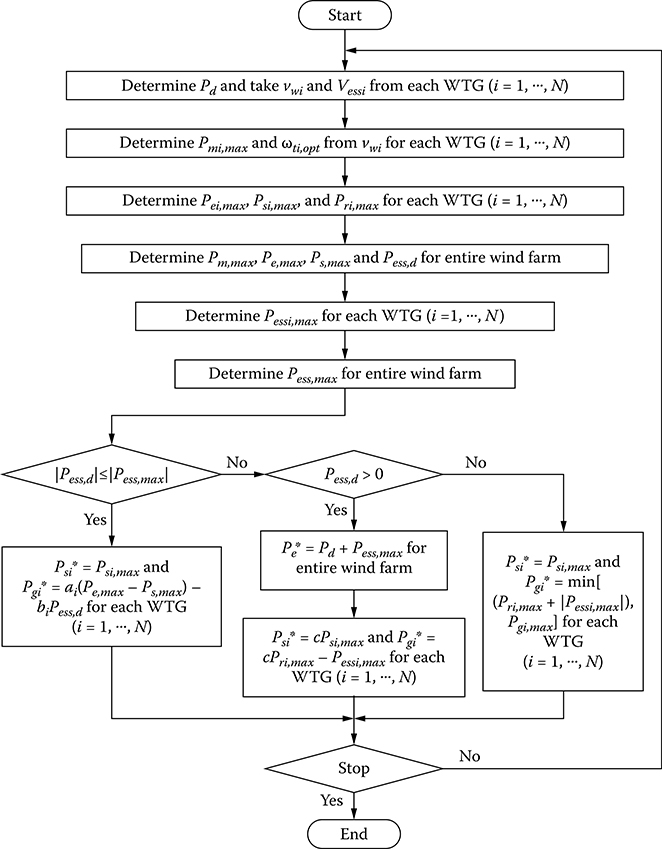
Figure 7.43 Flow chart of implementation of the WFSC.
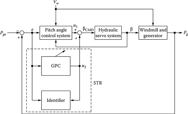
Figure 7.44 Pitch angle control system using GPC.
In this context, output power leveling of WTG for all operating regions by pitch angle control is discussed. The method presents a control strategy based on the average wind speed and standard deviation of wind speed and the pitch angle control, using GPC in all operating regions for WTG. The output power command is determined by approximate equation for windmill output using average wind speed. The output power of WTG for all operating regions is leveled by GPC, which is based on output power command. Thus the WTG is capable of providing stability operation for rapid change in operating point. And with this method it is possible to level output power of WTG for all operating regions by pitch angle control. Moreover, this pitch angle control can be used regardless of the kind of generators such as a permanent magnet synchronous generator (PMSG), a synchronous generator (SG), and DFIG.
The pitch angle control system using a GPC is shown in Figure 7.44, where Pgo(k) is output power command, Pg(k) is output power, e(k) is output power error of generator, u2(k) is control input of self-tuning regulator (STR), and k is number of sampling. The windmill and generator system is shown in Figure 7.45. Figure 7.46 shows the pitch angle control system that resolves pitch angle command βCMD, where output power error e is used as input into potential difference (PD) controller. The hydraulic servo system is shown in Figure 7.47. The system actually has nonlinear characteristics, but it is able to make a first-order lag system. The pitch angle command βCMD is limited by a limiter at the range of 10–90°.

Figure 7.45 System configuration of windmill and generator.

Figure 7.46 Pitch angle control system.
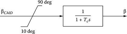
Figure 7.47 Hydraulic servo system.
The conventional method for the pitch angle law is fixed at more than cut-in wind speed and less than rated wind speed so that the output power for WTG is proportional to the fluctuation of wind speed at more than cut-in wind speed and less than rated wind speed. Thus, to achieve output power leveling of WTG for all operating regions by pitch angle control, the pitch angle control law has been extended as shown in Figure 7.48, whereas the fixed rated output power command has been converted to variable output power command.

Figure 7.48 Pitch angle control law for all operating regions.
7.8 Chapter Summary
This chapter deals with fluctuation minimization of power, frequency, and voltage by energy storage devices, especially using SMES systems. Various energy storage systems are discussed. A comparison among energy storage systems is also done. A multimachine power system consisting of hydraulic generators, diesel generators, and a fixed-speed wind generator is considered. The performance of the SMES is evaluated by considering their different load demands and energy capacities. Also, an attempt is made to evaluate the power and energy ratings of SMES systems. The required SMES power rating is analyzed using the standard deviation of frequency fluctuations with respect to the LPF time constant. From the simulation results, the following points are noteworthy.
By using the SMES system, the system frequency fluctuations are successfully minimized, and the frequency is maintained almost at the level of the nominal value of 60 Hz for different load demands.
The SMES can successfully minimize voltage fluctuations and can smooth the transmission line power.
The larger the capacity of the SMES is, the better the ability of fluctuations minimization of frequency, power, and voltage becomes. However, if a large-size SMES is adopted, its installation cost increases. Thus, the SMES capacity for fluctuations minimization of power, frequency, and voltage should be selected considering the viewpoint of cost-effectiveness.
If a 120 sec LPF time constant is selected and an SMES unit with a 55% power rating of that of the wind generator is adopted, a suitable reference value for the compensating power can be obtained and then sufficient smoothing effect can be achieved.
The required energy storage capacity of the SMES system is estimated under wind power fluctuations with various periodic wave forms. As a result, it is shown that the energy storage capacity can be obtained by the product of the wind farm power rating and the LPF time constant, and finally it is confirmed from simulation results that this estimation is valid.
Furthermore, this chapter discusses the output power leveling of wind generator systems by pitch angle control, power quality improvement by flywheel energy storage system, and constant power control of DFIG wind turbines with supercapacitor energy storage.
References
1. P. F. Ribeiro, B. K. Johnson, M. L. Crow, A. Arsoy, and Y. Liu, “Energy storage systems for advanced power applications,” Proceedings of the IEEE, vol. 89, no. 12, pp. 1744–1756, December 2001.
2. M. H. Ali, J. Tamura, and B. Wu, “SMES strategy to minimize frequency fluctuations of wind generator system,” Proceedings of the 34th Annual Conference of the IEEE Industrial Electronics Society (IECON 2008), November 10–13, 2008, Orlando, FL, pp. 3382–3387.
3. T. Asao, R. Takahashi, T. Murata, J. Tamura, M. Kubo, Y. Matsumura, et al., “Evaluation method of power rating and energy capacity of superconducting magnetic energy storage system for output smoothing control of wind farm,” Proceedings of the 2008 International Conference on Electrical Machines, pp. 1–6, 2008.
4. T. Asao, R. Takahashi, T. Murata, J. Tamura, M. Kubo, A. Kuwayama, et al., “Smoothing control of wind power generator output by superconducting magnetic energy storage system,” Proceedings of the 2007 International Conference on Electrical Machines, pp. 1–6, 2007.
5. H. J. Boenig and J. F. Hauer, “Commissioning tests of the Bonneville Power Administration 30 MJ superconducting magnetic energy storage unit,” IEEE Trans. Power Apparatus and Systems, vol. PAS-104, no. 2, pp. 302–309, February 1985.
6. S. C. Tripathy, M. Kalantar, and R. Balasubramanian, “Dynamics and stability of wind and diesel turbine generators with superconducting magnetic energy storage on an isolated power system,” IEEE Trans. Energy Conversion, vol. 6, no. 4, pp. 579–585, December 1991.
7. M. D. Mufti, R. Balasubramanian, S. C. Tripathy, and S. A. Lone, “Modelling and control of weak power systems supplied from diesel and wind,” International Journal of Power and Energy Systems, vol. 23, no. 1, pp. 24–36, 2003.
8. S. Nomura, Y. Ohata, T. Hagita, H. Tsutsui, S. Tsuji-Iio, and R. Shimada, “Wind farms linked by SMES systems,” IEEE Trans. Applied Superconductivity, vol. 15, no. 2, pp. 1951–1954, June 2005.
9. F. Zhou, G. Joos, C. Abbey, L. Jiao, and B. T. Ooi, “Use of large capacity SMES to improve the power quality and stability of wind farms,” IEEE Power Engineering Society General Meeting, 2004, vol. 2, pp. 2025–2030, June 2004.
10. M. H. Ali, M. Park, L.-K. Yu, T. Murata, and J. Tamura, “Improvement of wind generator stability by fuzzy logic-controlled SMES,” Proceeding of the International Conference on Electrical Machines and Systems 2007 (ICEMS 2007), pp. 1753–1758, October 8–11, 2007.
11. M. H. Ali, T. Murata, and J. Tamura, “Minimization of fluctuations of line power and terminal voltage of wind generator by fuzzy logic-controlled SMES,” International Review of Electrical Engineering (IREE), vol. 1, no. 4, pp. 559–566, October 2006.
12. T. Kinjo, T. Senjyu, N. Urasaki, and H. Fujita, “Terminal-voltage and output-power regulation of wind-turbine generator by series and parallel compensation using SMES,” IEE Proc.-Gener. Transm. Distrib., vol. 153, no. 3, pp. 276–282, May 2006.
13. J. J. Skiles, R. L. Kustom, K.-P. Ko, V. Wong, K.-S. Ko, F. Vong, et al., “Performance of a power conversion system for superconducting magnetic energy storage (SMES),” IEEE Trans. Power Systems, vol. 11, no. 4, pp. 1718– 1723, November 1996.
14. S. C. Tripathy and K. P. Juengst, “Sampled data automatic generation control with superconducting magnetic energy storage in power systems,” IEEE Trans. Energy Conversion, vol. 12, no. 2, pp. 187–192, June 1997.
15. IEEE Task Force on Benchmark Models for Digital Simulation of FACTS and Custom–Power Controllers, T&D Committee, “Detailed modeling of super-conducting magnetic energy storage (SMES) system,” IEEE Trans. Power Delivery, vol. 21, no. 2, pp. 699–710, April 2006.
16. PSCAD/EMTDC manual, Manitoba HVDC Research Center, 1994.
17. S. Roy, O. P. Malik, and G. S. Hope, “A k-step predictive scheme for speed control of diesel driven power plants,” IEEE Trans. Industry Applications, vol. 29, no. 2, pp. 389–396, March–April 1993.
18. G. S. Stavrakakis and G. N. Kariniotakis, “A general simulation algorithm for the accurate assessment of isolated diesel–wind turbines systems interaction. Part 1: A general multimachine power system model,” IEEE Trans. Energy Conversion, vol. 10, no. 3, pp. 577–583, September 1995.
19. G. N. Kariniotakis and G. S. Stavrakakis, “A general simulation algorithm for the accurate assessment of isolated diesel–wind turbines systems interaction. Part 2: Implementation of the algorithm and case-studies with induction generators,” IEEE Trans. Energy Conversion, vol. 10, no. 3, pp. 584–590, September 1995.
20. S. Roy, O. P. Malik, and G. S. Hope, “An adaptive control scheme for speed control of diesel driven power-plants,” IEEE Trans. Energy Conversion, vol. 6, no. 4, pp. 605–611, December 1991.
22. S. Heier, Grid integration of wind energy conversion system, John Wiley & Sons, 1998.
23. P. M. Anderson and A. Bose, “Stability simulation of wind turbine systems,” IEEE Trans. Power Apparatus and Systems, vol. PAS-102, no. 12, pp. 3791–3795, December 1983.
24. R. Dugan and T. McDermott, “Distributed generation,” IEEE Industry Applications Magazine, vol. 8, no. 2, pp. 19–25, March–April 2002.
24. P. Chiradeja and R. Ramakumar, “An approach to quantify the technical benefits of distributed generation,” IEEE Transactions on Energy Conversion, vol. 19, no. 4, pp. 764–773, December 2004.
25. F. Blaabjerg, R. Teodorescu, M. Liserre, and A. Timbus, “Overview of control and grid synchronization for distributed power generation systems,” IEEE Transactions on Industrial Electronics, vol. 53, no. 5, pp. 1398–1407, October 2006.
26. H. Nikkhajoei and R. Lasseter, “Distributed generation interface to the CERTS microgrid,” IEEE Transactions on Power Delivery, vol. 24, no. 3, pp. 1598–1608, July 2009.
27. F. Katiraei, R. Iravani, N. Hatziargyriou, and A. Dimeas, “Microgrids management,” IEEE Power & Energy Magazine, pp. 54–65, May–June 2008.
28. D. Salomonsson and A. Sannino, “Low-voltage DC distribution system for commercial power systems with sensitive electronic loads,” IEEE Transactions on Power Delivery, vol. 22, no. 3, pp. 1620–1627, July 2007.
29. P. Tsao, M. Senesky, and S. R. Sanders, “An integrated flywheel energy storage system with homopolar inductor motor/generator and high frequency drive,” IEEE Transactions on Industry Applications, vol. 39, no. 6, pp. 1710– 1725, November–December 2003.
30. J.-D. Park, C. Kalev, and H. Hofmann, “Control of high-speed solid rotor synchronous reluctance motor/generator for flywheel-based uninterruptible power supplies,” IEEE Transactions on Industrial Electronics, vol. 55, no. 8, pp. 3038–3046, February 2008.
31. H. Akagi and H. Sato, “Control and performance of a doubly-fed induction machine intended for a flywheel energy storage system,” IEEE Transactions on Power Electronics, vol. 17, no. 1, pp. 109–116, August 2002.
32. R. Cardenas, R. Pena, G. Asher, and J. Clare, “Control strategies for enhanced power smoothing in wind energy systems using a flywheel driven by a vector-controlled induction machine,” IEEE Transactions on Industrial Electronics, vol. 48, no. 3, pp. 625–635, June 2001.
33. X.-D. Sun, K.-H. Koh, B.-G. Yu, and M. Matsui, “Fuzzy-logic-based V/f control of an induction motor for a DC grid power-leveling system using fly-wheel energy storage equipment,” IEEE Transactions on Industrial Electronics, vol. 56, no. 8, pp. 3161–3168, May 2009.
34. R. Cardenas, R. Pena, G. Asher, J. Clare, and R. Blasco-Gimenez, “Control strategies for power smoothing using a flywheel driven by a sensorless vector-controlled induction machine operating in a wide speed range,” IEEE Transactions on Industrial Electronics, vol. 51, no. 3, pp. 603–614, June 2004.
35. X. Feng, J. Liu, and F. Lee, “Impedance specifications for stable DC distributed power systems,” IEEE Transactions on Power Electronics, vol. 17, no. 2, pp. 157–162, March 2002.
36. H. Mosskull, J. Galic, and B. Wahlberg, “Stabilization of induction motor drives with poorly damped input filters,” IEEE Transactions on Industrial Electronics, vol. 54, no. 5, pp. 2724–2734, October 2007.
37. R. Piwko, D. Osborn, R. Gramlich, G. Jordan, D. Hawkins, and K. Porter, “Wind energy delivery issues: Transmission planning and competitive electricity market operation,” IEEE Power Energy Mag., vol. 3, no. 6, pp. 47–56, November–December 2005.
38. L. Landberg, G. Giebel, H. A. Nielsen, T. Nielsen, and H. Madsen, “Short term prediction—An overview,” Wind Energy, vol. 6, no. 3, pp. 273–280, July– September 2003.
39. J. P. Barton and D. G. Infield, “Energy storage and its use with intermittent renewable energy,” IEEE Trans. Energy Conversion, vol. 19, no. 2, pp. 441–448, June 2004.
40. C. Abbey and G. Joos, “Supercapacitor energy storage for wind energy applications,” IEEE Trans. Ind. Appl., vol. 43, no. 3, pp. 769–776, May–June 2007.
41. B. S. Borowy and Z. M. Salameh, “Dynamic response of a stand-alone wind energy conversion system with battery energy storage to wind gust,” IEEE Trans. Energy Conversion, vol. 12, no. 1, pp. 73–78, March 1997.
42. M.-S. Lu, C.-L. Chang, W.-J. Lee, and L. Wang, “Combining the wind power generation system with energy storage equipments,” IEEE Trans. Ind. Appl., vol. 45, no. 6, pp. 2109–2115, November–December 2009.
43. W. Qiao, W. Zhou, J. M. Aller, and R. G. Harley, “Wind speed estimation based sensorless output maximization control for a wind turbine driving a DFIG,” IEEE Trans. Power Electron., vol. 23, no. 3, pp. 1156–1169, May 2008.
44. W. Qiao, G. K. Venayagamoorthy, and R. G. Harley, “Real-time implementation of a STATCOM on a wind farm equipped with doubly fed induction generators,” IEEE Trans. Ind. Appl., vol. 45, no. 1, pp. 98–107, January–February 2009.
45. S. Vazquez, S. M. Lukic, E. Galvan, L. G. Franquelo, and J. M. Carrasco, “Energy storage systems for transport and grid applications,” IEEE Trans. Industrial Electronics, vol. 57, no. 12, pp. 3881–3895, December 2010.
46. E. Manla, A. Nasiri, C. H. Rentel, and M. Hughes, “Modeling of zinc bromide energy storage for vehicular applications,” IEEE Trans. Ind. Electron., vol. 57, no. 2, pp. 624–632, February 2010.
47. D. P. Scamman, G. W. Reade, and E. P. L. Roberts, “Numerical modeling of a bromide-polysulphide redox flow battery. Part 1: Modelling approach and validation for a pilot-scale system,” J. Power Sources, vol. 189, no. 2, pp. 1220– 1230, April 2009.
48. D. P. Scamman, G. W. Reade, and E. P. L. Roberts, “Numerical modeling of a bromide-polysulphide redox flow battery. Part 2: Evaluation of a utility-scale system,” J. Power Sources, vol. 189, no. 2, pp. 1231–1239, April 2009.
49. S. Lemofouet and A. Rufer, “A hybrid energy storage system based on compressed air and supercapacitors with maximum efficiency point tracking (MEPT),” IEEE Trans. Ind. Electron., vol. 53, no. 4, pp. 1105–1115, June 2006.
50. D. J. Swider, “Compressed air energy storage in an electricity system with significant wind power generation,” IEEE Trans. Energy Conversion, vol. 22, no. 1, pp. 95–102, March 2007.
51. M. B. Camara, H. Gualous, F. Gustin, and A. Berthon, “Design and new control of DC/DC converters to share energy between supercapacitors and batteries in hybrid vehicles,” IEEE Trans. Veh. Technol., vol. 57, no. 5, pp. 2721–2735, September 2008.
52. H. Yoo, S. K. Sul, Y. Park, and J. Jeong, “System integration and power flow management for a series hybrid electric vehicle using supercapacitors and batteries,” IEEE Trans. Ind. Appl., vol. 44, no. 1, pp. 108–114, January– February 2008.
53. L. Shuai, K. A. Corzine, and M. Ferdowsi, “A new battery/ultracapacitor energy storage system design and its motor drive integration for hybrid electric vehicles,” IEEE Trans. Veh. Technol., vol. 56, no. 4, pp. 1516–1523, July 2007.
54. W. Henson, “Optimal battery/ultracapacitor storage combination,” J. Power Sources, vol. 179, no. 1, pp. 417–423, April 2008.
55. K. Jin, X. Ruan, M. Yang, and M. Xu, “A hybrid fuel cell power system,” IEEE Trans. Ind. Electron., vol. 56, no. 4, pp. 1212–1222, April 2009.
56. M. H. Todorovic, L. Palma, and P. N. Enjeti, “Design of a wide input range DC– DC converter with a robust power control scheme suitable for fuel cell power conversion,” IEEE Trans. Ind. Electron., vol. 55, no. 3, pp. 1247–1255, March 2008.
57. M. Ortuzar, J. Moreno, and J. Dixon, “Ultracapacitor-based auxiliary energy system for an electric vehicle: Implementation and evaluation,” IEEE Trans. Ind. Electron., vol. 54, no. 4, pp. 2147–2156, August 2007.
58. O. Briat, J. M. Vinassa, W. Lajnef, S. Azzopardi, and E. Woirgard, “Principle, design and experimental validation of a flywheel-battery hybrid source for heavy-duty electric vehicles,” IET Elect. Power Appl., vol. 1, no. 5, pp. 665– 674, September 2007.
59. T. Ise, M. Kita, and A. Taguchi, “A hybrid energy storage with a SMES and secondary battery,” IEEE Trans. Appl. Supercond., vol. 15, no. 2, pp. 1915–1918, June 2005.
60. T. Senjyu, R. Sakamoto, N. Urasaki, T. Funabashi, H. Fujita, and H. Sekine, “Output power leveling of wind turbine generator for all operating regions by pitch angle control,” IEEE Trans. Energy Conversion, vol. 21, no. 2, pp. 467– 475, June 2006.
61. E. Muljadi and C. P. Butterfield, “Pitch-controlled variable-speed wind turbine generation,” IEEE Trans. Ind. Appl., vol. 37, no. 1, pp. 240–246, January– Februar 2001.
62. J. L. Rodriguez-Amenedo, S. Arnalte, and J. C. Burgos, “Automatic generation control of a wind farm with variable speed wind turbines,” IEEE Trans. Energy Conversion, vol. 17, no. 2, pp. 279–284, June 2002.
63. A. Miller, E. Muljadi, and D. S. Zinger, “A variable speed wind turbine power control,” IEEE Trans. Energy Conversion, vol. 12, no. 2, pp. 181–186, June 1997.
64. P. Ledesma and J. Usaola, “Doubly fed induction generator model for transient stability analysis,” IEEE Trans. Energy Conversion, vol. 20, no. 2, pp. 388–397, June 2005.
65. C. Carrillo, A. E. Feijóo, J. Cidrás, and J. González, “Power fluctuations in an isolated wind plant,” IEEE Trans. Energy Convers., vol. 19, no. 1, pp. 217–221, March 2004.
66. Jae-Do Park, “Simple flywheel energy storage using squirrel-cage induction machine for DC bus microgrid systems,” Proceedings of the 36th Annual Conference on IEEE Industrial Electronics Society, IECON 2010, 7-10 Nov. 2010, pp. 3040-3045, Glendale, AZ, USA.
67. L. Qu and W. Qiao, “Constant power control of DFIG wind turbines with supercapacitor energy storage,” IEEE Trans. Industry Applications, vol. 47, no. 1, pp. 359–367, January/February 2011.