
Analyzing routing protocol traffic
Analyzing overlay traffic
Analyzing Routing Protocol Traffic
So far, we have learned how to set up Wireshark, perform packet captures, and analyze Layer 2 to Layer 4 traffic. Most of the traffic that we have looked at so far is data traffic. When we are dealing with packet loss in the network, we usually try to understand the problem based on what is happening in the network: Is there an errored link in the network dropping the traffic? Is network congestion leading to data loss? When the data loss is happening in the network, chances are high that the data might also be control plane traffic. Although we can give separate treatment to the control plane traffic from the data traffic using QoS, that only helps prioritizing packets on the device, not on the wire. So, a packet loss can simply drop data traffic as well as control plane traffic. Thus, a control plane flap due to any amount of packet loss can still be analyzed using the methods that we have seen so far. It could also be the case, though, that control plane protocols misbehave even when there is no packet loss or congestion in the network. This chapter is focused on analyzing control plane traffic and understanding the headers and functionality of various routing protocols, diving deeper into certain cases and how we can troubleshoot them using Wireshark. Note that this chapter does not focus on teaching any control plane or data plane traffic, but just analyzing different control plane and data plane traffic, which can prove useful for network engineers. It is assumed that network engineers are well aware of the protocols discussed in this chapter.
OSPF
Open Shortest Path First (OSPF), defined in RFC 2328, is one of the well-known and most widely adopted interior gateway protocols (IGPs). It is a dynamic routing protocol that operates within a single autonomous system (AS) and is suitable for large heterogeneous networks. OSPF uses the Dijkstra algorithm, also known as the shortest path first (SPF) algorithm, to calculate the shortest path to the destination. In OSPF, the shortest path to a destination is calculated based on the cost of the route, which considers variables such as bandwidth, delay, and load.
Backbone area: Network segment that belongs to area 0.0.0.0. All other areas are either physically or virtually connected to the backbone area. Exchanging routing information between multiple nonzero or nonbackbone areas is only possible through the backbone area.
Standard nonzero area: In this area, OSPF packets are normally transmitted. This area is directly or virtually connected to the backbone area.
Stub area: This area does not allow and accept routes from external sources such as routes learned by other routing protocols and redistributed into OSPF.
Totally stubby area: This area does not accept routes from external sources and link information from other areas. Instead, a default route is advertised in this area for allowing the router in this area to reach a destination in other areas or even external sources.
Not so stubby area (NSSA): An NSSA is derived from a stub area with the difference that this area also has an Autonomous System Boundary Router (ASBR) router attached to it and learns the external routes from the redistribution happening on the ASBR.
Backbone router: A backbone router runs OSPF and has at least one interface part of the backbone area or area 0.0.0.0.
Internal router: An internal router has OSPF adjacency only with the devices in the same area. These routers do not form adjacency across multiple areas.
Area Border Router (ABR): An ABR router forms OSPF neighbor adjacency with multiple devices in multiple areas. Because it has adjacency in multiple areas, it maintains a copy of the link-state topology database of multiple areas and distributes it to the backbone area.
ASBR: An ASBR router participates in other routing protocols apart from OSPF and exchanges the routing information learned from other protocols into OSPF and vice versa.
Router LSA (Type 1)
Network LSA (Type 2)
Summary LSA (Type 3)
Summary ASBR LSA (Type 4)
AS External LSA (Type 5)
NSSA LSA (Type 7)
OSPF Area to LSA Mapping
Area Type | LSAs Allowed |
|---|---|
Backbone area | Type 1, 2, 3, 4, 5 |
Standard or normal area | Type 1, 2, 3, 4, 5 |
Stub area | Type 1, 2, 3 |
Totally stubby area | Type 1, 2, and Type 3 default route |
NSSA | Type 1, 2, 3, 7 |
Totally NSSA | Type 1, 2, 7, and Type 3 default route |
Broadcast
Nonbroadcast
Point-to-point
Point-to-multipoint
Down: This is the initial state of an OSPF router where no information is exchanged between the routers.
Attempt: This state is similar to the down state, with the difference that the router is in the state of initiating a conversation. This state is only applicable for nonbroadcast multiaccess (NBMA) networks.
Init: – In this state, a Hello packet has been received from the neighbor router, but the two-way communication has not yet been established.
2-Way: Indicates that a bidirectional conversation has been established between two routers. After this state, DR/BDR is elected for broadcast and NBMA networks. A router on a broadcast or NBMA network becomes full with the DR/BDR, but remains in 2-way with all the remaining routers.
Exstart: In this state DR/BDR is established as a master–subordinate relationship. The router with the highest router ID is selected as the master and starts exchanging the link-state information.
Exchange: In this state, the OSPF neighbors exchange database description (DBD) packets. The DBD packets contain LSA headers that describe the contents of the LSDB and are compared with the router’s LSDB.
Loading: If there is any discrepancy or missing information found by comparing the DBD packets with the LSDB, routers send link-state request packets to the neighbor routers. In response to the link-state requests, the neighbor router responds with LS Update packets that are acknowledged by the receiving router using LSA packets.
Full: In this state, the router’s database is completely synchronized with the LSDB of the neighbor routers and the routers become fully adjacent.

OSPF Hello packet

OSPF Hello packet with active neighbor
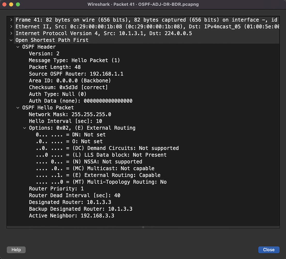
OSPF Hello packet with DR/BDR
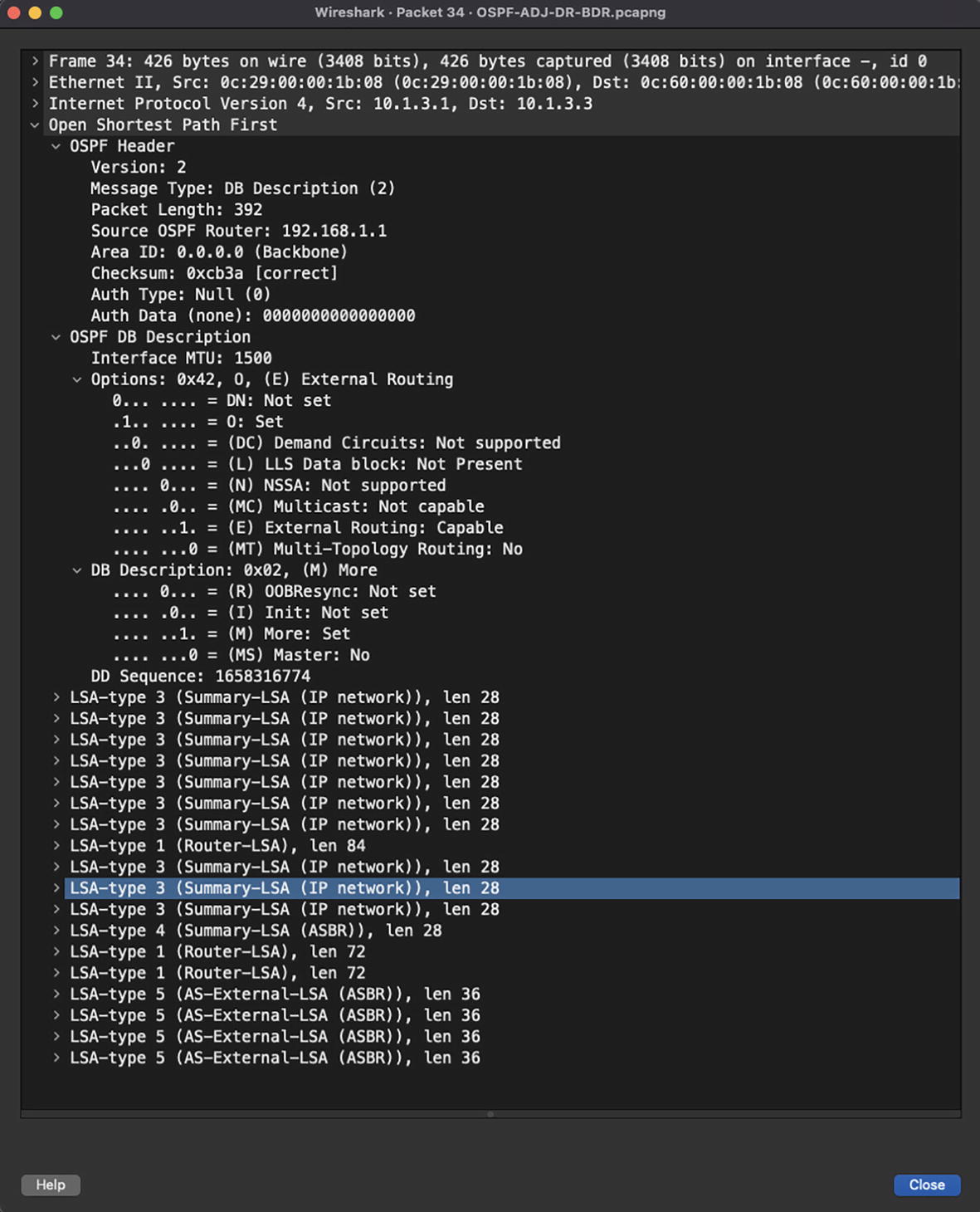
OSPF database description packet
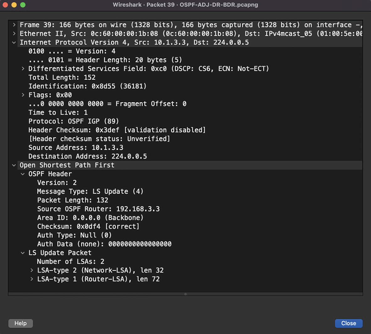
OSPF LS Update packet
LS Age (2 bytes): Represents the elapsed time since the LSA was created.
Options (1 byte): Used for advertising OSPF capabilities supported by the router.
LS Type (1 byte): Indicates the type of LSA.
Link State ID (4 bytes): Indicates the link of either the router or the network the link represents.
Advertising Router (4 bytes): Indicates the OSPF router ID of the router originating the LSA.
LS Sequence Number (4 bytes): A sequence number used to detect old or duplicate LSAs.
LS Checksum (2 bytes): Checksum of the LSA, which is used for identifying any data corruption.
Length (2 bytes): Length of the LSA including 20 bytes of the header.
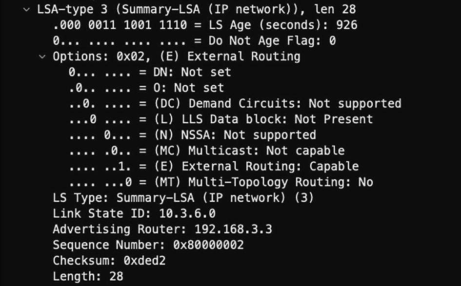
OSPF LSA header

OSPF LSA packet

OSPF NSSA Hello packet

OSPF Type 7 LSA
Wireshark OSPF Filtering
Filter | Description |
|---|---|
ospf.area_id == 0.0.0.10 | Filters OSPF packets for specified Area ID |
ospf.advrouter == 192.168.5.5 | Filters OSPF packets with the specified router ID of the advertising router |
ospf.hello | Filters OSPF Hello packets |
ospf.lsa.router | Filters OSPF router LSA |
ospf.lsa.network | Filters OSPF network LSA |
ospf.lsa.summary | Filters OSPF summary LSA |
ospf.lsa.nssa | Filters for NSSA (Type 7) LSA |
ospf.lsa.asext | Filters for Type 5 (External) LSA |
EIGRP
Establishing communication: EIGRP uses a three-way handshake for establishing communication.
Exchanging routes: EIGRP uses reliable transport for exchanging routes.
Performing path computation: The procotol leverages the DUAL algorithm to perform path computation.
Installing routes in the Routing Information Base (RIB): EIGRP only installs loop-free paths in the RIB.
One of the key components of EIGRP is its Topology table. It contains all known paths, locally learned routes, and externally learned routes (learned via redistribution). The information available in the Topology table is used by the DUAL algorithm to calculate the loop-free paths. The EIGRP Topology table not only contains information about the paths, but it also maintains information about when a route was withdrawn by a neighbor.
Hello
Update
Acknowledge
Query
Reply
Let’s take a closer look at these packets one by one.
Hello Packet

EIGRP Hello packet
The Hello packet also has the Stub flag set when sent by an EIGRP stub router. Users can filter it in Wireshark using the filter eigrp.stub_flags.
Update Packet

EIGRP full update

EIGRP partial update
Users can filter EIGRP update packets in Wireshark using the eigrp.opcode == 1 filter. This filter displays both full and partial updates in EIGRP.
Acknowledge Packet

EIGRP Acknowledge packet
You can filter the EIGRP Acknowledge packet by using the Wireshark filter (eigrp.opcode == 5_ && !(eigrp.ack == 0). The ! operator ensures that we only capture the Acknowledge packet and not the EIGRP Hello packet.
Query Packet
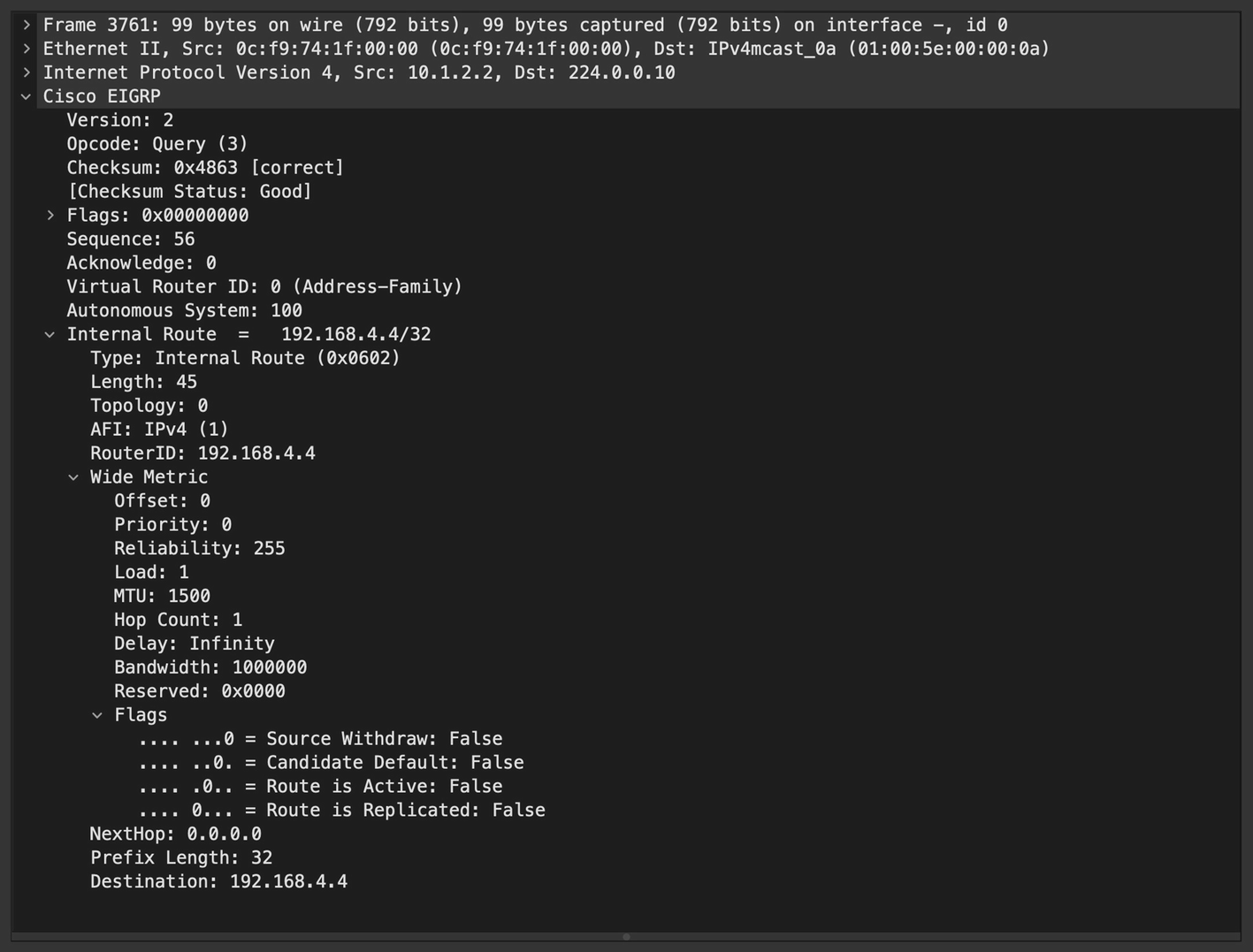
EIGRP Query packet
You can filter the EIGRP Query packet in Wireshark using the filter eigrp.opcode == 3.
EIGRP Query packets are not sent to stub routers.
Reply Packet
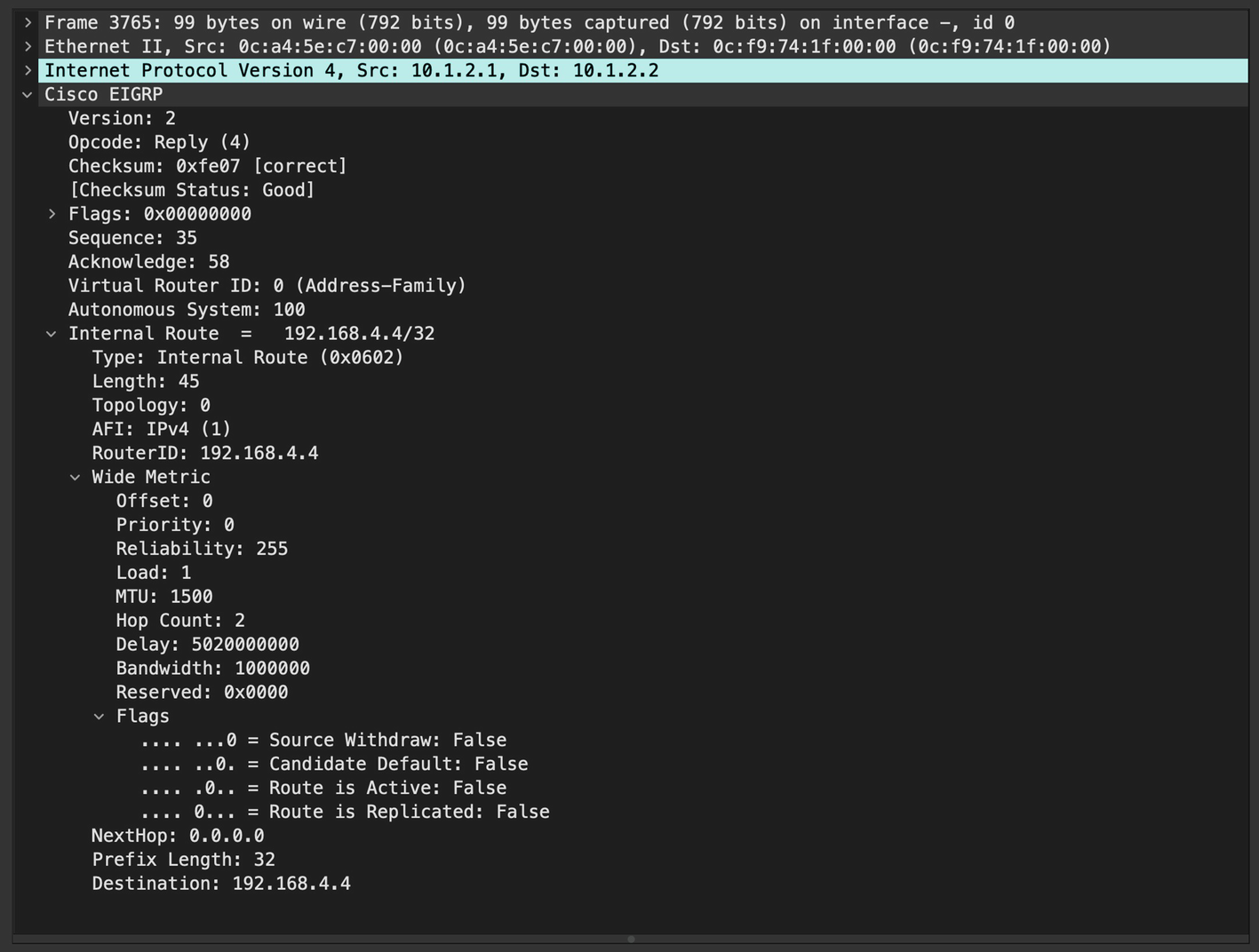
EIGRP Reply packet
BGP
BGP, often called the routing protocol of the Internet, is an open standard protocol used for connecting network across different AS boundaries. BGP is a highly scalable protocol and has support for multiple address families such as IPv4, IPv6, VPNv4, L2VPN, EVPN, and so on, which allows BGP to be the protocol of choice in enterprise, datacenter, and service provider environments. BGP, in general, cannot route traffic on its own. It leverages the information from IGP to reach to the next hop for the prefix. BGP knows about the prefixes that might be within the same AS boundary or across multiple AS boundaries. BGP only knows about next hops to reach the destination, but it needs IGP to get to that next hop.
Internet BGP (iBGP): BGP peering established with other routers within the same AS boundary.
External BGP (eBGP): BGP peering established with routers across AS boundaries.
Idle: In this state, BGP detects a start event and initializes the BGP resources on the router. The BGP process initiates a TCP connection toward the peer.
Connect: In this state, BGP waits for the three-way handshake to complete. If the three-way handshake is successful, an OPEN message is sent and the BGP process moves to the OpenSent state. If it is not successful, BGP moves to the Active state, and waits for a ConnectRetry timer.
Active: BGP starts a new three-way handshake. If the connection is successful, it moves to OpenSent state. If it is unsuccessful, the BGP process moves back to the Connect state.
OpenSent: In this state, the BGP process sends an OPEN message to the remote peer and waits for an OPEN message from the peer.
OpenConfirm: In this state, the router has already received the OPEN message from the remote peer and is now waiting for a KEEPALIVE or NOTIFICATION message. On receiving the KEEPALIVE message, the BGP session is established. On receiving a NOTIFICATION message, BGP moves to the Idle state.
Established: This state indicates that the BGP session is established and is now ready to exchange routing updates via the BGP UPDATE message.
- OPEN: This is the first message exchanged between BGP peers after a three-way handshake has been established between the peers. Once each side confirms the information shared in the BGP OPEN message, other messages are exchanged between them. The following information is compared as part of the OPEN message:
BGP version
Source IP of the OPEN message should match with configured peer IP
Received AS number should match the configured remote AS number of the BGP peer
BGP Router ID must be unique
Other security parameters such as password, TTL, and so on
KEEPALIVE: The BGP KEEPALIVE message acts like a Hello packet to check whether the BGP peer is alive or not. This message is used to keep sessions from expiring.
NOTIFICATION: BGP NOTIFICATION is sent when the BGP process encounters an error condition. When this message is received, the BGP process closes the active session for which the notification was received. The NOTIFICATION message also contains the information such as error code and suberror code that can be used to determine the cause of the error condition.
UPDATE: This message is used for exchanging routing updates (advertisements and withdrawals) between BGP peers.
Marker: Set to fffffffffffffffffffffff.
Length: Length of the BGP header
Type (OPEN message): Value set to 1.
Version: Specifies the current BGP version used by the router. The current version is 4 as defined in RFC 4271.
MS AS: Specifies the AS number of the router originating the OPEN message.
Hold Time: Specifies the Hold Timer value set on the router sending the OPEN message.
BGP Identifier: Router ID of the router sending the OPEN message.
Optional Parameters Length: Variable length, specifies the combined length of all the parameters included in the Optional Parameters field.
- Optional Parameters: This field is used by the router to advertise optional BGP capabilities that are supported in BGP by the OS running on the advertising router. Some of these capabilities include the following:
Multiprotocol BGP (MP-BGP) support
Route Refresh support
4-octet (4-byte) AS number support

BGP OPEN message
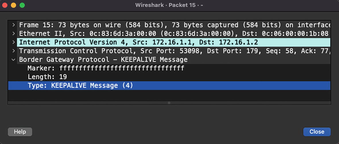
BGP KEEPALIVE message
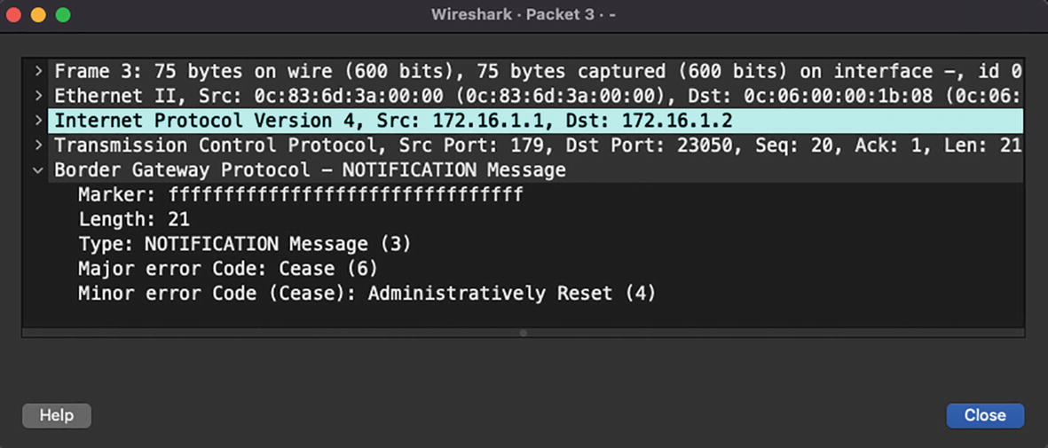
BGP NOTIFICATION message

BGP UPDATE message
TCP session
Packet loss
Network OS not generating packets in a timely manner
Device not sending the BGP packets out in a timely manner
BGP updates getting corrupted
PIM
Source address : Unicast address of a multicast source or sender.
Group address : Destination IP address of a multicast group. Note that multicast addresses range from 224.0.0.0 to 239.255.255.255.
Multicast distribution tree (MDT) : Multicast flows from source to receivers over an MDT. The MDT is either shared or dedicated based on the multicast implementation
Rendezvous point (RP) : A multicast-enabled router that acts as the root of the shared MDT.
Protocol Independent Multicast (PIM) : Routing protocol used to create MDTs.
First-hop router (FHR) : First L3 hop that is directly adjacent to the multicast source.
Last-hop router (LHR) : First L3 hop that is directly adjacent to the receivers.
In this chapter, we focus on the PIM protocol and its messages and see how it is used to build MDT.
Dense mode: – Based on a push model, PIM Dense mode operates under the assumption that receivers are densely dispersed through the network. In this mode, multicast traffic is flooded domain-wide to build a shortest path tree, and the branches are pruned back where no receivers are found.
Sparse mode: Based on a pull model, PIM Sparse mode assumes that the receivers are sparsely dispersed. In this mode, PIM neighbors are formed and traffic is forwarded only over the PIM-enabled path. Using PIM messages, the join request from receivers is forwarded to the RP and thus the mechanism is known as explicit join. Because of this method, it is also the most preferred and widely used method for multicast distribution.
PIM Version (4 bits): Version number is set to 2.
Type (4 bits): Used to specify the PIM message type.
Reserved (8 bits): Reserved for future use. The value is set to 0 in this field during transmission and is ignored by the PIM neighbor.
Checksum (16 bits): Used to calculate the checksum of the entire PIM message except for the payload section.
PIM message types
Type | Message Type | Destination Address | Description |
|---|---|---|---|
0 | Hello | 224.0.0.13 | Neighbor discovery. |
1 | Register | Address of RP (unicast) | Register message is sent by FHR to RP to register the source. |
2 | Register-stop | Address of FHR (unicast) | This message is sent by RP to the FHR in response to the PIM Register message. |
3 | Join/Prune | 224.0.0.13 | Join or prune from an MDT. |
PIM Hello Message
PIM Hello Message Options
Option Type | Option Value |
|---|---|
1 | Holdtime: The amount of time in which the neighbor is in a reachable state |
2 | Has the following parts: • LAN Prune Delay: Delay before transmitting Prune message in a shared LAN segment • Interval: Time interval for overriding a Prune message • T: Join message suppression capability |
19 | DR priority used during DR election |
20 | Generation ID: Random number indicating neighbor status |
24 | Address List: used for informing neighbors about secondary IP address on interface |
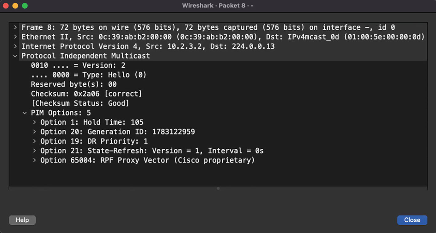
PIM Hello message
PIM Register Message
Type: Value is set to 1 for Register message.
Border (B-bit): The PIM multicast border router functionality is defined in RFC 4601, which designates a local source when this bit is set to 0 and designates the source in a directly connected cloud when this bit is set to 1.
Null-Register: This bit is set to 1 when a Null-Register message is sent. In the Null-Register message, the FHR only encapsulates the header from the source and not the complete encapsulated data packet of the multicast stream coming from the source.
Multicast Data packet: The original multicast packet sent by the source is encapsulated inside the PIM Register message. If the message is a Null-Register message, only a dummy IP header containing the source and group address is encapsulated in the PIM Register message. Note that the TTL of the original packet decrements before encapsulation into the PIM Register message.
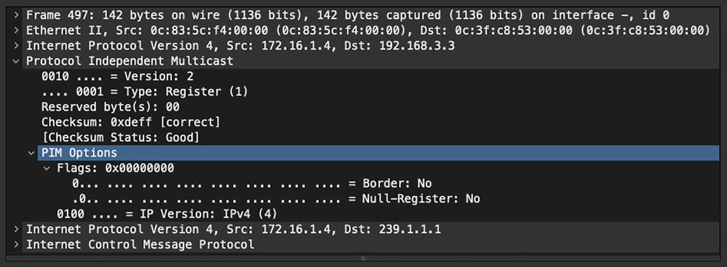
PIM Register message
PIM Register-Stop Message
Type: Value is set to 2 for PIM Register-stop message.
Group Address: Group address of the encapsulated multicast packet in the PIM Register message.
Source Address: Source address of the encapsulated multicast packet in the PIM Register message.

PIM Register-stop message
PIM Join/Prune Message
Type: Value is set to 3 for Join/Prune message.
Upstream Address: Address of the upstream neighbor to which the message is targeted. It also has subfields that represent the address family of the upstream neighbor as well as the encoding.
Number of Groups: Represents the number of multicast group sets in the message.
Holdtime: The amount of time to keep the Join/Prune state alive.
Num Joins: Number of joined sources in the message.
- Joined Source Address {IP Address x.x.x.x/32}
Sparse bit (S): Set to 1 for PIM Sparse mode.
Wildcard bit (W): When set to 1, this represents wildcard a in the (*, G) entry. When set to 0, this indicates that the encoded source address for (S, G) entry.
RP bit (R): When set to 0, join is sent toward source. When set to 1, join is sent toward RP.
Num Prunes: Number of pruned sources in the message.
Pruned Source Address {IP Address x.x.x.x/32}: Represents the list of sources being pruned for the group. All three flags in Joined Source Address are applicable for Pruned Source Address, too.
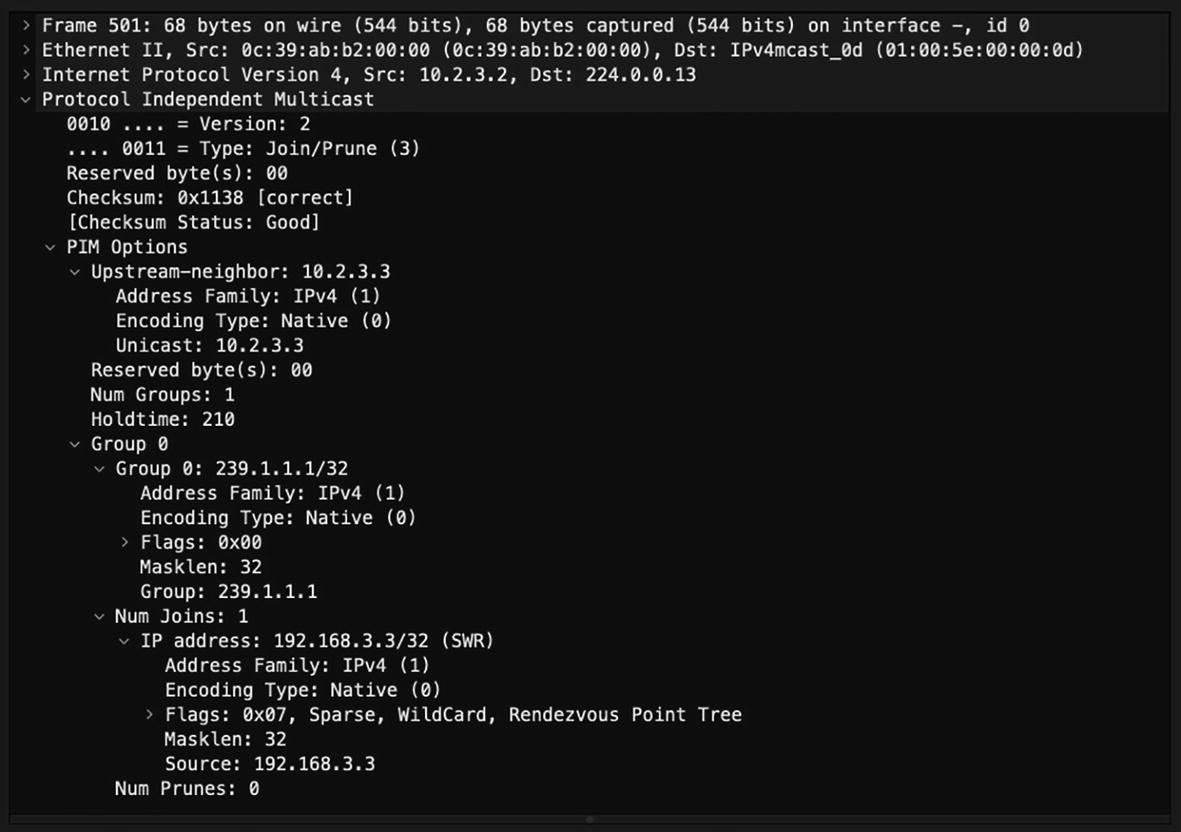
PIM Join message
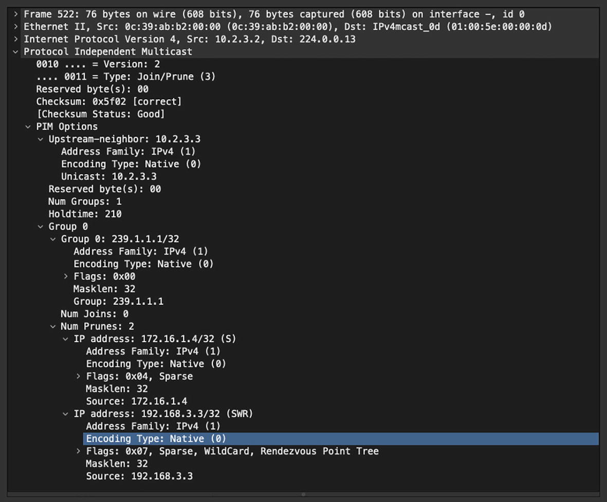
PIM Prune message
Analyzing Overlay Traffic
So far, we have learned about analyzing routing protocol traffic that can run on physical links or virtual links such as SVIs. Such networks are known as underlay networks. The routing protocols, however, can also run over an overlay network. An overlay network is a network that is built on top of another network and leverages underlying network configuration and protocols to establish communication as if they were locally connected. The devices or endpoints in an overlay network could be residing multiple hops away in the same or a different geographical location. In overlay traffic, the actual host traffic is encapsulated with the headers of the underlay network. We next look at different overlay protocols and how we can analyze the overlay traffic using Wireshark.
GRE
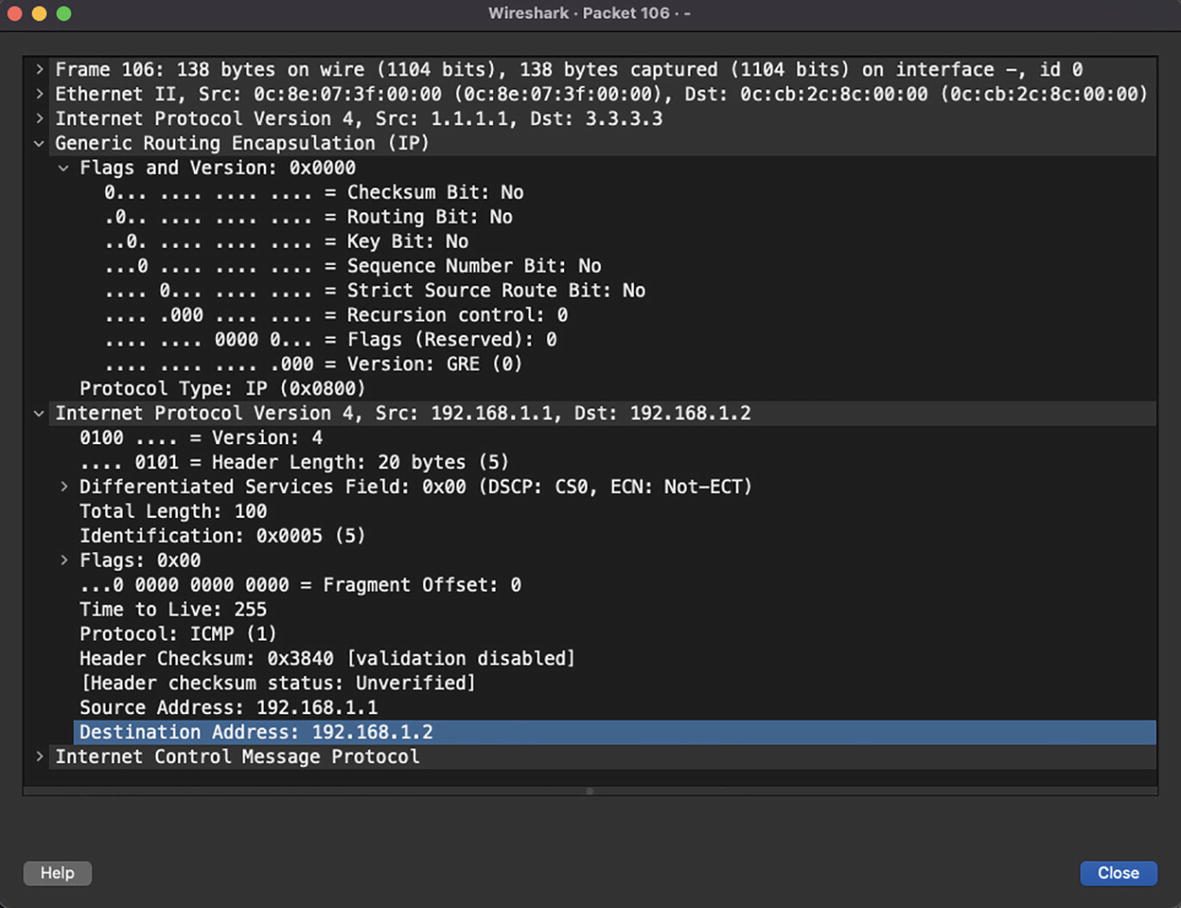
GRE encapsulation

GRE encapsulated traffic after first Layer 3 hop
IPSec
Authentication Headers (AH) : AH provides data integrity, authentication, and antireplay capabilities, which protects against unauthorized transmission of packets.
- Internet Key Exchange (IKE) : – IKE is a network security protocol that defines how to dynamically exchange encryption keys and use Security Associations (SAs) to establish shared security attributes between the two IPSec tunnel endpoints. The Internet Security Association Key Management Protocol (ISAKMP) provides a framework for authentication and key exchange and defines how to setup SAs. There are two versions of IKE:
IKEv1
IKEv2
Encapsulating Security Payload (ESP) : ESP provides authentication for the payload or data. It ensures data integrity, encryption, and authentication and prevents any replay attacks on the payload.

Wireshark capture of IPSec IKEv1 negotiations

Wireshark capture of first Phase 1 packet

Wireshark capture of second Phase 1 packet

Wireshark capture of DH keys

Wireshark capture of Phase 1 authentication process

Wireshark capture of Phase 2 Quick mode
Once Phase 2 is completed, the IPSec tunnels are formed, and all the packets exchanged over the tunnel interface are encrypted. For instance, if you send ICMP traffic, looking at the Wireshark capture you might not be able to identify that it is an ICMP packet or some other type of packet.
VXLAN
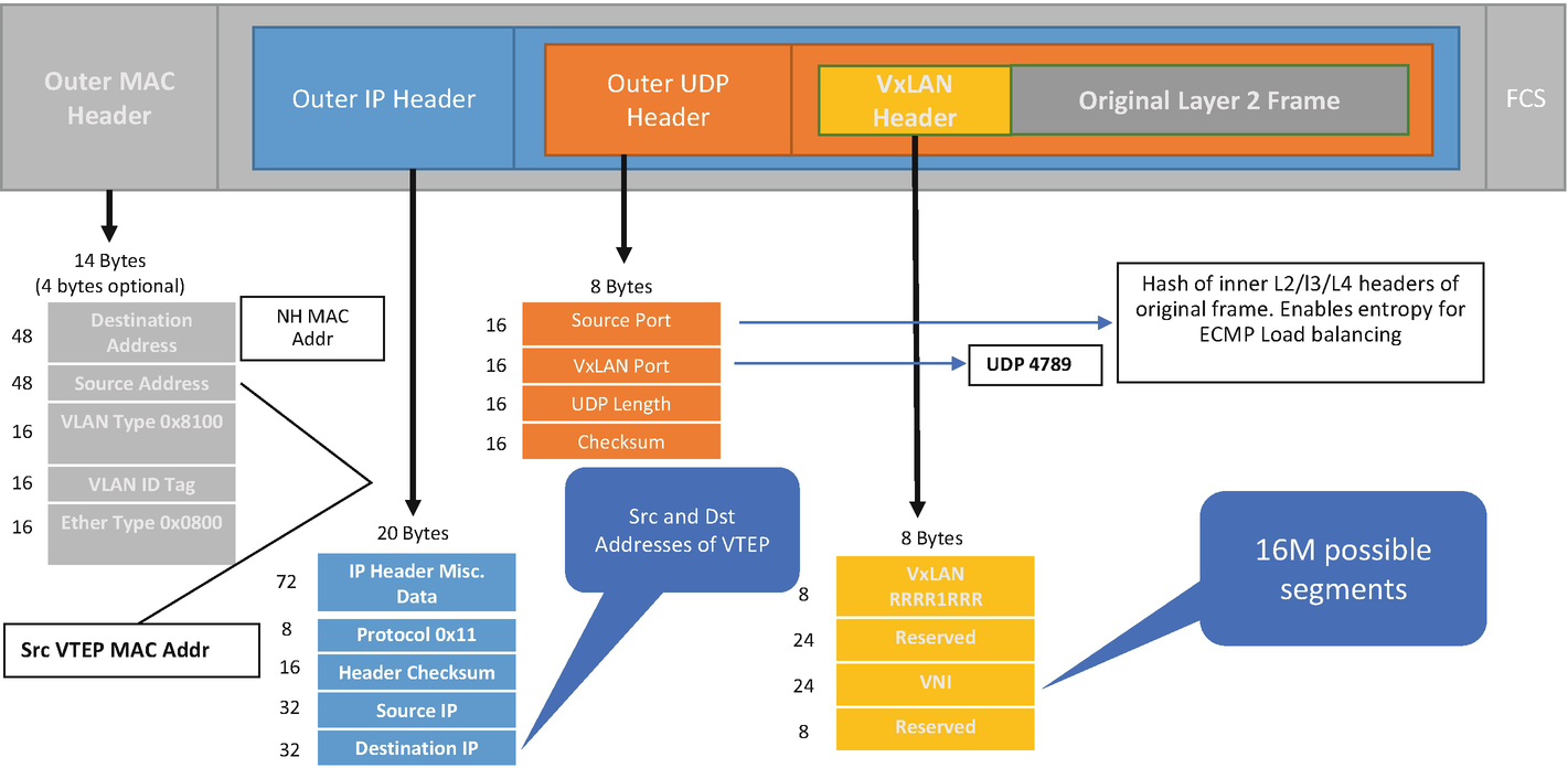
VXLAN encapsulated Ethernet frame
The VXLAN encapsulation and de-encapsulation is done by Virtual Tunnel End Points (VTEPs) that connect classic Ethernet segments to the VXLAN fabric. The VXLAN core fabric is usually based on a spine-leaf architecture. Traffic forwarding in VXLAN fabric is dependent on the type of traffic. Broadcast, Unknown Unicast, and Multicast (BUM) traffic requires either multicast replication or unicast replication of packets to a remote VTEP as these packets are sent to multiple VTEPs at the same time. Unicast traffic, on the other hand, does not require any kind of replication. Unicast traffic is encapsulated with VXLAN and a UDP header and sent to the destination VTEP where the host resides. There are, thus, two types of replication methods supported with VXLAN.
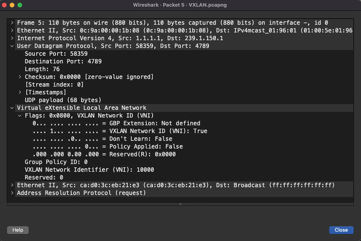
VXLAN encapsulation BUM traffic with multicast replication
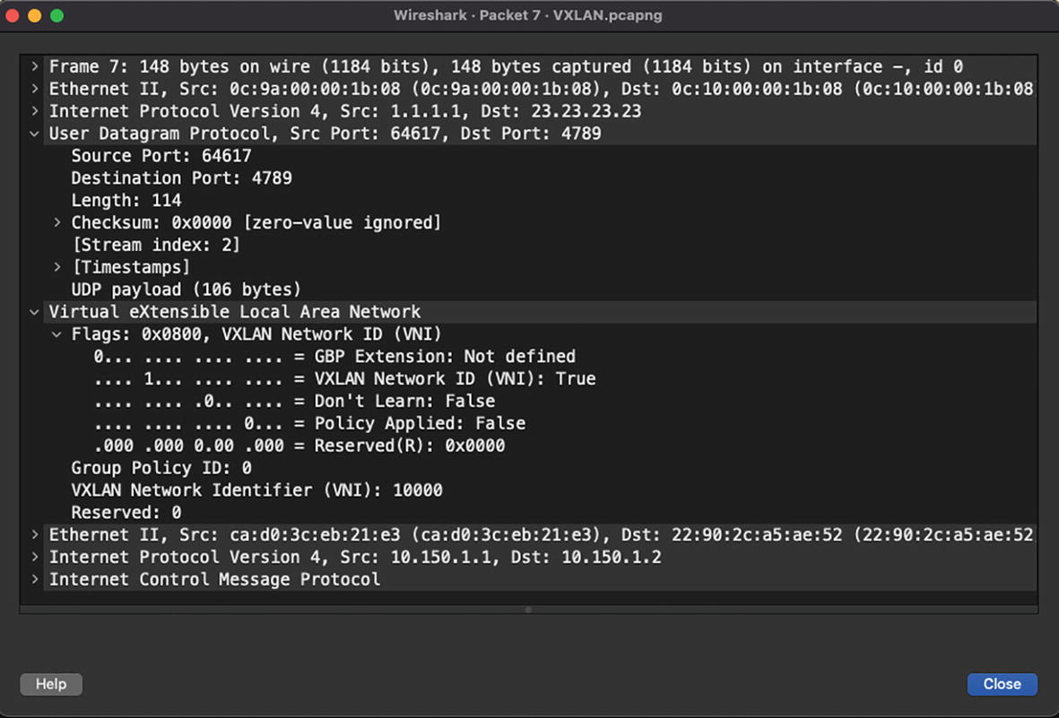
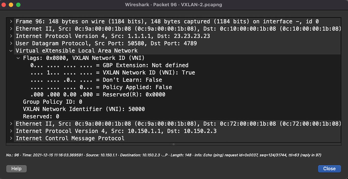
VXLAN encapsulated unicast packet
The second replication method is ingress replication, or unicast replication. This method is used in scenarios where either the organization is not interested in enabling multicast in its fabric or the devices are incapable of running multicast features. The BUM traffic, in this case, is replicated to statically configured remote VTEPs as unicast packets.
So far, we have explored the communication of hosts within the same VNI. Inter-VNI communication in VXLAN fabric is performed through symmetrical Integrated Routing and Bridging (IRB) and with the help of a Layer 3 VNI. For some context of what a Layer 3 or Layer 2 VNI is, let’s first understand the concept of a tenant. A tenant is a logical instance that provides Layer 2 or Layer 3 services in a datacenter. Each tenant consists of multiple Layer 2 VNIs and a Layer 3 VNI. Layer 2 VNIs are the segments where the hosts are connected and the Layer 3 VNI is used for inter-VNI routing.
Typical LAN
There are various implementations of VXLAN such as VXLAN-EVPN and VXLAN Multi-site, but the concept remains the same and the method of encapsulation and de-encapsulation remains the same. Thus, when investigating any VXLAN issue, you might run into issues related to BUM replication or unicast forwarding. In the case of BUM replication with multicast, you might want to troubleshoot the issue from a multicast perspective more than from a VXLAN perspective.
Summary
This chapter is primarily focused on topics that are specific to network engineers to assist them in day-to-day troubleshooting of various routing protocols and overlay network traffic. We began the chapter learning about how to analyze routing protocol traffic such as OSPF, EIGRP, BGP, and PIM. We then moved on to learn about overlay traffic such as GRE and IPSec VPNs. As part of analyzing overlay traffic, we also covered one of the most widely used and critical encapsulations, VXLAN. This chapter assumes that readers understand how these protocols work. They can then build on top of that to reach a deeper understanding of those protocols by learning about the content of their headers and how they can troubleshoot some scenarios that are commonly seen in production environments.