Layer 2 frames
Layer 3 packets
Analyzing QoS markings
Layer 2 Frames
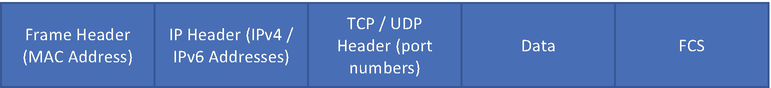
Data encapsulation with different headers
At each layer, the data are encapsulated in a specific format known as the packet data unit (PDU). The PDU defines the structure or format in which the data will be shared with the layer above or layer beneath the current layer. The PDU could simply be the data, a segment (at the Transport layer), a packet (at the Network layer), a frame (at the Data Link layer), or even bits.
Media Access Control (MAC) : Controls access to the network medium by interfacing with the network adapter. It is responsible for flow control and multiplexing device transmissions over the network.
Logical Link Control (LLC) : LLC provides error control and flow control over the physical medium. It is also used for identifying line protocols.
Layer 2 Protocols
Protocol | Description |
|---|---|
Cisco Discovery Protocol (CDP) | CDP is a Cisco proprietary protocol that is primarily used to exchange information between directly connected Cisco devices. |
Link Layer Discovery Protocol (LLDP) | LLDP is a vendor-neutral Layer 2 discovery protocol that is commonly used by devices to advertise information to their directly connected devices. |
Point-to-Point Protocol (PPP) | PPP provides the standard mechanism for transmitting data over point-to-point links. |
Frame Relay | Frame Relay is a packet-switched WAN protocol that operates over the Physical and Data Link layers. |
Asynchronous Transfer Mode (ATM) | ATM is a cell-switched WAN protocol that is designed to facilitate various types of traffic streams. |
Ethernet | Ethernet is the most widely used Data Link layer protocol used in both LAN and WAN environments. |
There are several other protocols that are used at Layer 2, but most of them are now obsolete or have very limited implementation. In this chapter, we focus on Ethernet frames.
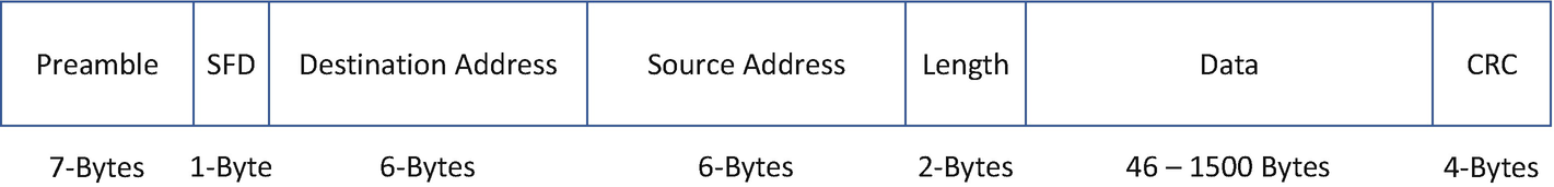
Ethernet Frames
Preamble: Ethernet frame starts with a 7-byte Preamble field. Initially this field was introduced to allow for loss of a few bits due to signal delays, but high-speed Ethernet links do not require the Preamble field.
Start of frame delimiter (SFD) : SFD is a 1-byte field that is always set to 10101011. This field indicates the start of the frame.
Destination Address (DA) : DA is a 6-byte field that holds the destination MAC address of the machine.
Source Address (SA) : SA is also a 6-byte field that holds the source MAC address of the machine from which the packet originated.
Length: This 2-byte field indicates the length of the entire Ethernet frame.
Data: The Data section holds the payload of the frame. Note that both the IP header and data will be inserted into this section if IP is being used over Ethernet. The minimum length of the data field is 46 bytes, and the maximum data can be as long as 1,500 bytes, assuming the interface maximum transmission unit (MTU) is set to 1,500. If the data length is less than the minimum length of 46 bytes, then 0s are padded to meet the minimum possible data length.
Cyclic Redundancy Check (CRC) : The checksum is computed based on the 32-bit hash code generated using the destination address, source address, length, and data field of the frame and stored in the CRC field. If the checksum computed by the source or sender is not the same as that of the client or receiving device, the data received seem corrupted.
802.3 Ethernet frame
Destination Address
Source Address
Type (EtherType)
Data (Variable size)
Frame Checksum (FCS)
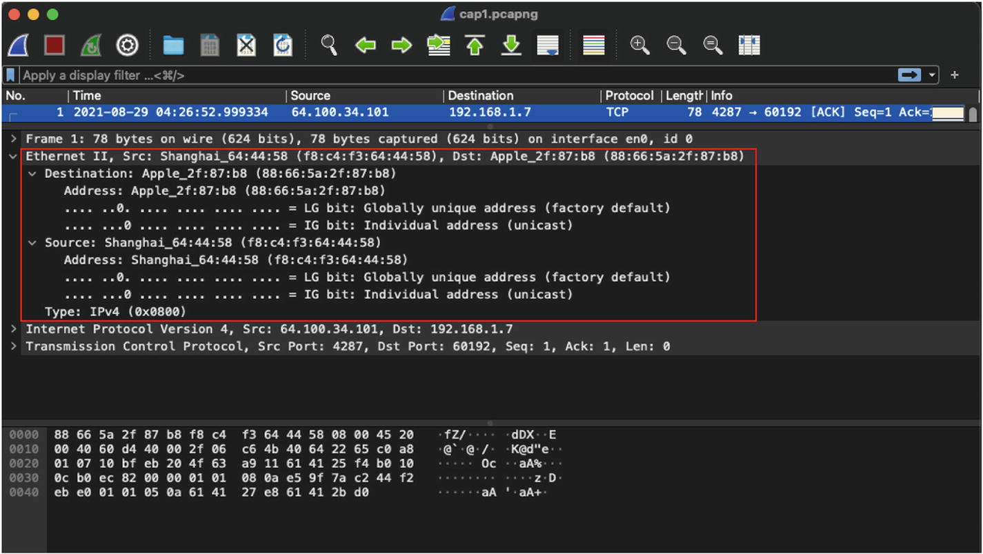
Ethernet II header in IPv4 packet
By default, FCS is not visible in the Wireshark capture. To view the FCS for the Ethernet header, go to Wireshark ➤ Preferences ➤ Protocols ➤ Ethernet and enable Assume Packets Have FCS option. Once that option is enabled, the Wireshark packet detail view will display the FCS field under the Ethernet II header.
Well-Known EtherTypes
EtherType | Protocol |
|---|---|
0x0800 | IPv4 |
0x0806 | ARP |
0x8100 | VLAN-Tagged Frame (IEEE 802.1Q) |
0x8847 | MPLS |
0x86DD | IPv6 |
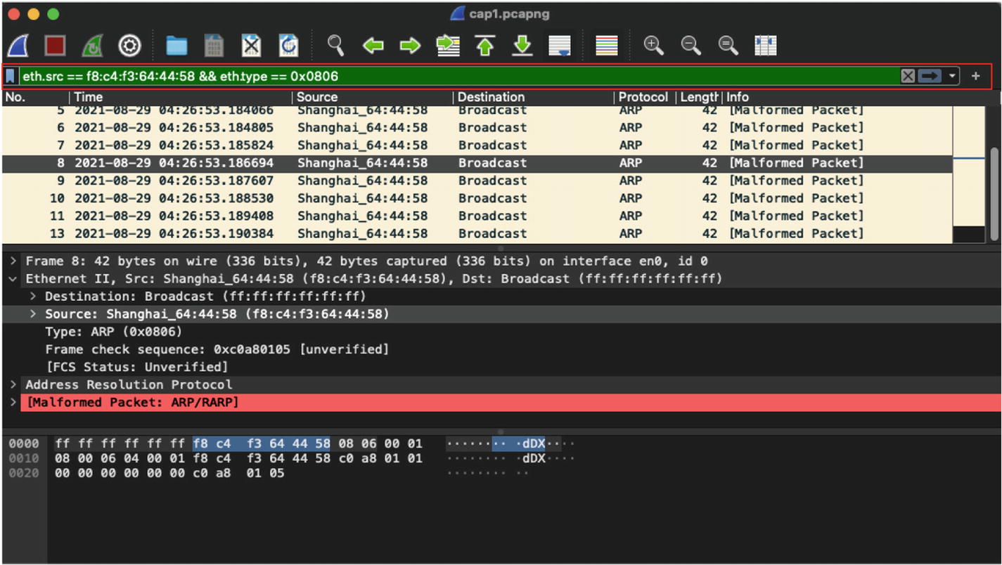
Filtering of broadcast frames sourced from a specific MAC address
Layer 3 Packets
When troubleshooting issues within a single broadcast domain or local LAN environments, Layer-2-based captures are more relevant, but when investigating issues that span multiple network segments that might be residing in different geographical location, we primarily focus on looking at Layer 3 and upper layer information in the packet captures. When talking about Layer 3 packets, we are primarily referring to either IPv4 packets or IPv6 packets. The protocols at Layer 3 provide logical addressing in a network (Internet or intranet) and ensure routing of data across different network segments. Even when dealing with tunneling technologies, the logical addressing of the tunnel interfaces and routing traffic across tunnel interfaces is still required. Before diving into IPv4 or IPv6 packets, let’s first understand ARP and its importance for establishing network communication.
Address Resolution Protocol
It is important to remember that both physical and logical addresses are required to establish communication in the network. Logical addresses allow users to establish communication across multiple network segments, and physical addresses are used for establishing communication within the same network segment. To forward traffic within the same broadcast segment, MAC addresses are required by the switch. Unless the switch knows about the MAC address of the host, it will not be able to forward the traffic toward the port where the destination host is connected. The MAC addresses of all the hosts connected to a switch within the same broadcast domain are stored in a Content Addressable Memory (CAM) table. If the MAC address of the destination address is not known, the switch will first perform a lookup in its cache. If the address is not found even in the cache, then a request is flooded to all the ports within the same broadcast domain until the MAC address is identified.
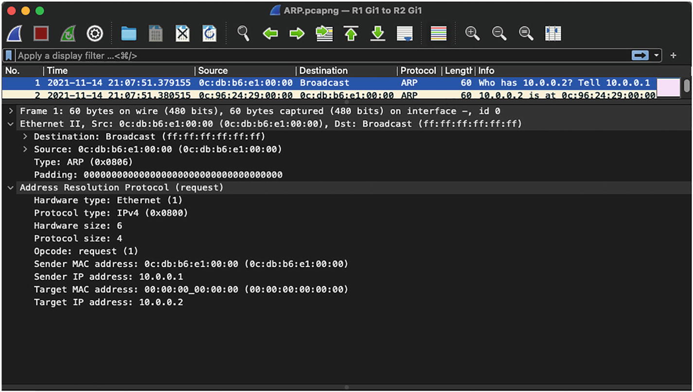
ARP request: An ARP request is basically a broadcast packet that is initiated by the sender or source host when it does not know the MAC address of the destination host or receiver.
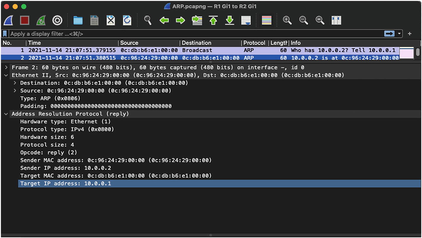
ARP response: When a host with the destination IP address for which the ARP request was sent receives the ARP request, it replies with an ARP response, which is basically a unicast packet directed toward the sender or the source host.

ARP request
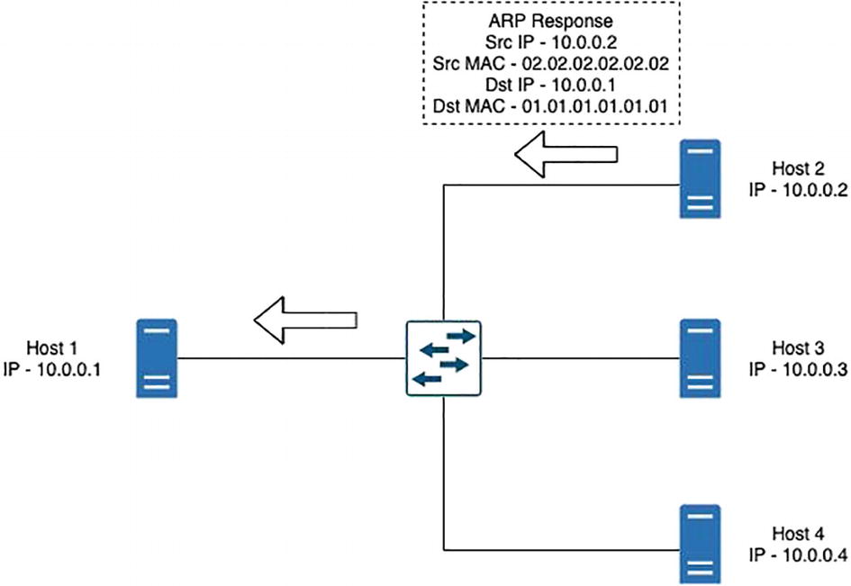
ARP response
IPv4 Packets
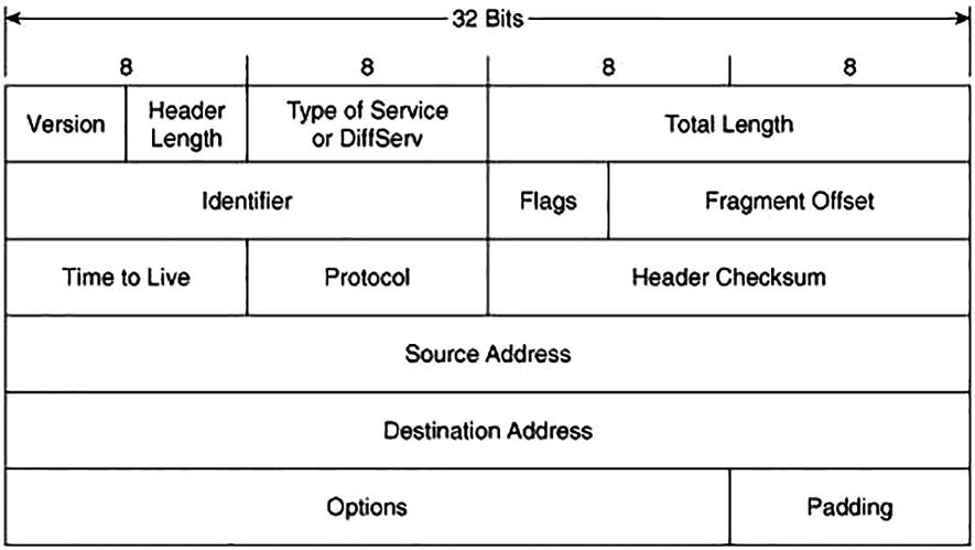
IPv4 header
Version: This 4-bit field indicates the IP version being used. There are devices that could be dual stack (support for IPv4 and IPv6 address) and the version field helps the device understand how to treat the traffic.
Internet Header Length (IHL) : This is a 4-bit field that contains the size of the IPv4 header. The 4 bits are used to specify the number of 32-bit words in the header. The minimum value of this field is 5 and the maximum value is 15, which basically indicates that the minimum IPv4 header length can be 20 bytes and the maximum can be 60 bytes.
Differentiated Services Code Point (DSCP) : This is a 6-bit field that was previously known as a Type of Service (ToS) field. This field specifies differentiated services (DiffServ), defined in RFC 2474, and it is used to provide service quality features such as Voice over IP (VoIP) calls or data streaming. Based on the values assigned in this field, different traffic streams are given different priority in the network and treated differently by routers and switches.
Explicit Congestion Notification (ECN) : ECN is a 2-bit field that allows for end-to-end network congestion notification without dropping packets. For the ECN feature to work, both endpoints are required to support this feature.
Total Length: This is a 16-bit field that defines the entire packet size in bytes including the header and payload. The minimum size is 20 bytes and the maximum size is 65,535 bytes.
Identification: The Identification field is used to identify a group of IP datagram packets uniquely and is also widely used for packet tracing purposes.
- Flags: This 3-bit field is used to control and identify fragments of an IP datagram. There are three possible values that are set in the Flags field:
Bit 0: Reserved
Bit 1: Do not fragment (also known as DF bit)
Bit 2: More fragments
Fragment Offset: This 13-bit field specifies the fragment offset relative to the start of the original unfragmented IP datagram in blocks. Each block is measured in units of 8 bytes. The maximum possible offset is 65,528 ((213 – 1) * 8).
Time to Live (TTL) : TTL is an 8-bit field that indicates the maximum time that a packet can live in an Internet system. The maximum value of TTL is 255 seconds and it is decremented when a packet is processed at each routed hop and forwarded to the next hop. If the TTL value is zero (0), the packet is discarded or dropped. This is to ensure that the packets do not keep looping in the Internet system.
Protocol: The 8-bit Protocol field is used to denote which protocol will be used in the data section of the datagram. For instance, the two most common protocol numbers that are usually seen in the network are protocol number 6, which is used to represent TCP, and protocol number 17, which represents a UDP packet. The protocol numbers are assigned and maintained by the Internet Assigned Numbers Authority (IANA).
Header Checksum: The 16-bit Header Checksum field in the IPv4 header is used for validating the integrity of the packet. When an IPv4 packet arrives at the router, the router calculates the checksum of the packet and compares it with the value in the this field. If the value matches, the packet is forwarded; otherwise, the packet is dropped.
Source Address (SA) : The 32-bit Source Address is used to specify the IPv4 address of the source device that originated the packet.
Destination Address (DA) : The 32-bit Destination Address field is used to specify the IPv4 address of the destination device to which the packet is destined.
- Options: The Options field is an optional field that is only set when the IHL value is greater than 5 (i.e., between 6 and 15). The Options field contains values and settings for security-related options and might be considered dangerous by some routers and dropped. You might see the Options field set when using the Record Route option with extended ICMP pings or for Timestamps. Table 3-3 shows the list of options that can be used in an IPv4 header and Table 3-4 displays the defined options for IPv4.Table 3-3
IPv4 Header Options
Field
Size (Bits)
Description
Copied
1
Set to 1 if the options need to be copied across all fragments of a fragmented packet
Option Class
2
0 – Control Options
1 – Reserved
2 – Debugging and Measurement
3 – Reserved
Option Number
5
Specifies an option
Option Length
8
Indicates the size of the entire option; might not be set for simple options
Option Data
Variable
Holds option specific data; might not be set for simple options
Data: The data or payload in the Data field is based on the value set in the Protocol field of IPv4 header. For instance, if the protocol number is set to 1, then the payload will contain ICMP-related data.
Defined Options for IPv4
Option Type (Decimal/Hexadecimal) | Option Name | Description |
|---|---|---|
0/0x00 | EOOL | End of Option List |
1/0x01 | NOP | No Operation |
2/0x02 | SEC | Security (defunct) |
7/0x07 | RR | Record Route |
10/0x0A | ZSU | Experimental Measurement |
11/0x0B | MTUP | MTU Probe |
12/0x0C | MTUR | MTU Reply |
15/0x0F | ENCODE | ENCODE |
25/0x19 | QS | Quick-Start |
30/0x1E | EXP | RFC 3692-style Experiment |
68/0x44 | TS | Timestamp |
82/0x52 | TR | Traceroute |
94/0x5E | EXP | RFC 3692-style Experiment |
130/0x82 | SEC | Security (RIPSO) |
131/0x83 | LSR | Loose Source Route |
133/0x85 | E-SEC | Extended Security (RIPSO) |
134/0x86 | CIPSO | Commercial IP Security Option |
136/0x88 | SID | Stream ID |
137/0x89 | SSR | Strict Source Route |
142/0x8E | VISA | Experimental Access Control |
144/0x90 | IMITD | IMI Traffic Descriptor |
145/0x91 | EIP | Extended Internet Protocol |
147/0x93 | ADDEXT | Address Extension |
148/0x94 | RTRALT | Router Alert |
149/0x95 | SDB | Selective Directed Broadcast |
151/0x97 | DPS | Dynamic Packet State |
152/0x98 | UMP | Upstream Multicast Packet |
158/0x9E | EXP | RFC 3692-style Experiment |
205/0xCD | FINN | Experimental Flow Control |
222/0xDE | EXP | RFC 3692-style Experiment |
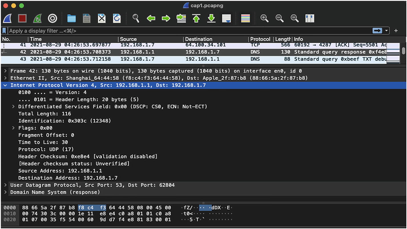
IPv4 header in Wireshark capture
IPv4 Addressing
Class A: 0.0.0.0 to 127.255.255.255
Class B: 128.0.0.0 to 191.255.255.255
Class C: 192.0.0.0 to 223.255.255.255
Class D (multicast addresses): 224.0.0.0 to 239.255.255.255
Class E (experimental addresses): 240.0.0.0 to 255.255.255.255
Public address: Public IPv4 addresses are the addresses that are uniquely identified on the Internet and are usually allocated to organizations by IANA.
- Private addresses: Private IPv4 addresses are primarily used in almost every organization for managing hosts in LAN environments. These addresses are not advertised in the global Internet routing table. The private IPv4 address range is shown here:
Class A private IP: 10.0.0.0 to 10.255.255.255
Class B private IP: 172.16.0.0 to 172.31.255.255
Class C private IP: 192.168.0.0 to 192.168.255.255
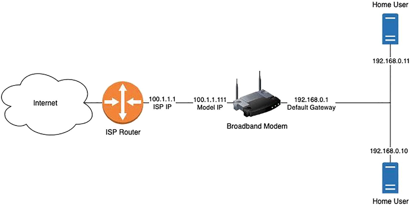
Home broadband Internet connection
Loopback addresses: 127.0.0.0 to 127.255.255.255
APIPA: 169.254.0.0 to 169.254.255.255
Limited broadcast: 255.255.255.255
ICMP
ICMPv4 used for IPv4
ICMPv6 used for IPv6
Type: 8-bit
Code: 8-bit
Checksum: 16-bit
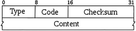
ICMP header
When sending an ICMP packet, the Protocol field within the IP header is set to a value of 1.
ICMP Echo Request and Echo Reply: The ICMP Echo Request has the Type/Code value of 8/0 and the ICMP Echo Reply has the Type/Code value of 0/0. The Echo Request and Echo Reply messages are used to validate the connectivity between the source and destination device in the network and are commonly used via the ICMP Packet InterNet Grouper (PING) tool. When the source device tries to verify the connectivity toward the destination device using the PING tool, it sends an ICMP request, and if the destination device is reachable, it responds back with the ICMP reply message.
- ICMP Redirect message: ICMP Redirect messages are used by routers on nonoptimal paths to notify hosts about the availability of an optimal path between the source and the destination. An ICMP Redirect message has the ICMP Type value of 5 and has four codes:
Code 0: Redirect datagram for the network
Code 1: Redirect datagram for the host
Code 2: Redirect datagram for the type of service and network
Code 3: Redirect datagram for the type of service and host
- ICMP Destination Unreachable message: If a router receives a datagram that it is unable to forward or deliver to the destination, it replies with an ICMP Destination Unreachable message. There can be multiple reasons for the router being unable to deliver the packet. The different reasons are covered under various ICMP codes. The ICMP Destination Unreachable message has the Type value of 3 and the following code options:
Code 0: Destination network unreachable
Code 1: Destination host unreachable
Code 2: Destination protocol unreachable
Code 3: Destination port unreachable
Code 4: Fragmentation required, and DF set
Code 5: Source route failed
Code 6: Destination network unknown
Code 7: Destination host unknown
Code 8: Source host isolated
Code 9: Network administratively prohibited
Code 10: Host administratively prohibited
Code 11: Network unreachable for type of service
Code 12: Host unreachable for type of service
Code 13: Administratively prohibited
- ICMP Time Exceeded message: This message is sent by the router to the source device or host if the TTL value reaches 0 before it reaches the destination. One reason that could cause the TTL to expire is that the destination router is more than 255 hops away or, alternatively, there is a routing loop in the network that has caused the TTL value to reach 0. The ICMP Time Exceeded message has the Type value of 11 and has the following codes:
Code 0: TTL expired
Code 1: Fragment reassembly time exceeded
ICMP Source Quench message: If a router receives a large amount of data that it can handle and it can send an ICMP Source Quench message to the sender asking it to slow down the rate at which it is sending the traffic. The ICMP Source Quench message has the Type and Code value set to 0/0.
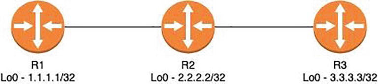
Network topology

Wireshark capture for ICMP request
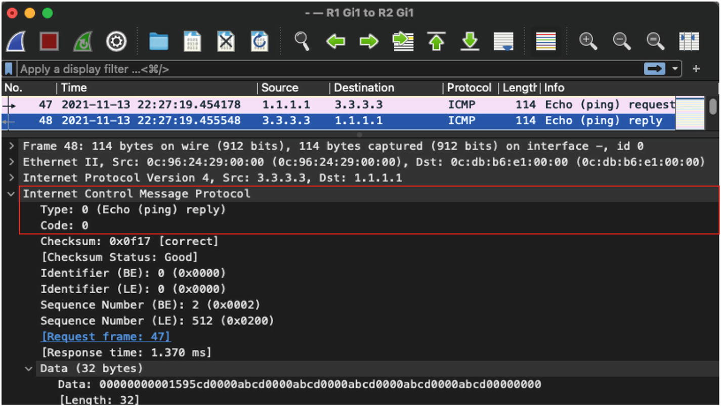
Wireshark capture for ICMP reply
Although in most cases you might not want to perform a packet capture for ICMP request and ICMP reply packets, in scenarios where even the ICMP packets are unreachable, you might want to perform packet capture to isolate the node that might be dropping the packets.
ICMP Ping with Record Route Option

Wireshark capture of ping packet with Record Route option
IP Fragmentation and Reassembly
Maximum segment size (MSS): Data payload
MTU – MSS + IP header (20 bytes) + TCP header (20 bytes)
So, if an interface MTU is set to a default valie of 1500, then the MSS will be calculated as follows:
MSS = 1500 (MTU) – 20 bytes (IP header) – 20 bytes (TCP header)

Wireshark capture of first fragmented packets
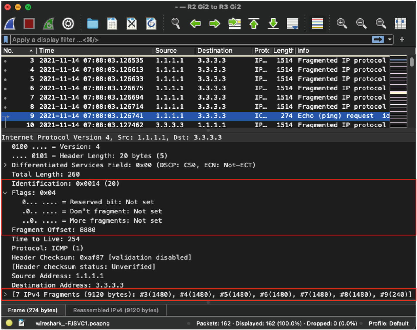
Wireshark capture of last fragmented packet
Nonfragmented
Initial fragment
Noninitial fragment
Fragment Settings in IP Header
Packet Type | More Fragments Flag | Fragment Offset Field |
|---|---|---|
Nonfragmented | 0 | 0 |
Initial fragment | 1 | 0 |
Noninitial fragment (not last) | 1 | Nonzero |
Noninitial fragment (last) | 0 | Nonzero |

Wireshark capture of ICMP Destination Unreachable message
IPv6 Packets
Streamlined header: Although the IPv6 header is much larger than the IPv4 header, several fields from the IPv4 header were removed in the IPv6 header, making it more streamlined.
- Revised fields: Some of the fields in the IPv6 header were revised when compared to Ipv4:
The TTL field in IPv4 was converted to the Hop Limit field in IPv6.
The Precedence and ToS fields were moved to the Traffic Class field.
The Protocol field was covered under the Next Header field.
The 32-bit Source Address and Destination Address fields were now converted to 128-bit Source Address and Destination Address fields.
Flow label: Flow label was introduced in the IPv6 header for identifying streams such as real-time traffic that required special treatment in the network.

IPv4 and IPv6 headers
Version: This 4-bit field indicates the IP version that is in use. For IPv6 packets, you will see the value set to 6.
- Traffic Class: This 8-bit field is used for allowing special treatment to a packet in the network based on the DSCP values assigned to an IPv6 packet. It is a combination of two fields:
TOS: The first 6 bits are used to set the DSCP value of a packet similar to an IPv4 packet. The DSCP value defaults to 0.
ECN: The last 2 bits of this field are used for congestion notification similar to how it is done in an IPv4 packet.
Flow Label: The 20-bit Flow Label field is used by a source to group a set of packets belonging to the same flow. It is usually used for QoS and to ensure the packets of same flow take the same path.
Payload Length: This 16-bit field represents the packet’s payload. The payload may not exceed 216 (65,535) bytes of data except in situations where extension headers are being used. When extension headers are used, the field value is set to 0.
Next Header: This 8-bit field indicates the higher layer protocol that follows the IPv6 header.
Hop Limit: The 8-bit Hop Limit field is similar to the TTL field in an IPv4 header. The value of this field represents the number of routed hops a packet can traverse before getting dropped or reaching the destination. The maximum value of this field is 255. At every routed hop, the value of the Hop Limit field is decreased by 1 and when the value reaches 0, the packet is dropped.
Source Address: The 128-bit Source Address field represents the IPv6 address of the sender from which the packet originated.
Destination Address: The 128-bit Destination Address field represents the IPv6 address of the packet’s destination.

Wireshark capture of IPv6 header
There is no option for fragmentation in the IPv6 header similar to the Flags or Fragment Offset fields in the IPv4 header. If fragmentation is required on Ipv6 packets, the Extensions header is used.
IPv6 Addressing
A deep dive on IPv6 addressing is outside the scope of this book. To learn more about IPv6 addressing, refer to RFC 4291.
Link local address: Link local addresses are automatically assigned to the interfaces on which IPv6 is enabled. These addresses are used to communicate with hosts on the same subnet. This address always starts with FE80.
Global unicast: These addresses are public IPv6 addresses that are uniquely recognized and are routable over the Internet.
Unicast address: A unicast address is used for a single host on a network.
Unique local: These addresses are routable within the administrative domain.
Multicast address: Multicast addresses are used to send data to multiple receivers who are subscribed to the multicast group address.
Anycast address: Anycast addresses are used to send data to multiple locations using the same IPv6 address. An anycast address is allocated for a set of interfaces that typically belong to different nodes.
Global unicast: 2000::/3
Unique local: FC00::/7
Link local: FE80::/10
Multicast: FF00::/8
Extension Headers

IPv6 header with Extension Headers
IPv6 Extension Headers and Next Header Values
Order | Header Type | Next Header Code |
|---|---|---|
1 | Basic IPv6 header | - |
2 | Hop-by-Hop options | 0 |
3 | Destination options (with Routing options) | 60 |
4 | Routing header | 43 |
5 | Fragment header | 44 |
6 | Authentication header | 51 |
7 | Encapsulation Security Payload header | 50 |
8 | Destination options | 60 |
9 | Mobility header | 135 |
No next header | 59 | |
Upper layer | TCP | 6 |
Upper layer | UDP | 17 |
Upper layer | ICMPv6 | 58 |
ICMPv6
Improved multicast routing
Extensions
Stateless Autoconfiguration (SLAAC)
The ICMPv6 header is similar an IPv4 header. It contains the Type, Code, and Checksum fields, followed by ICMPv6 options and contents that are based on type and code values.
In the previous section, you likely noticed that when we were talking about IPv6 addressing, we did not talk about broadcast. That is because there is no concept of broadcast in IPv6, as it is considered an inefficient mechanism. Because there is no broadcast, ARP cannot work for IPv6. This is where ICMPv6 comes into play. We talk about the IPv6 neighbor discovery process in the next section, but for now, let’s focus on the different ICMPv6 messages and their Type and Code values. The ICMPv6 messages are divided into two categories, error messages and informational messages.
ICMPv6 Error Messages
Type | Header Type | Code | Definition |
|---|---|---|---|
1 | Destination unreachable | 0 | No route to destination |
1 | Communication with destination administratively prohibited | ||
2 | Beyond scope of source address | ||
3 | Address unreachable | ||
4 | Port unreachable | ||
5 | Source address failed ingress/egress policy | ||
6 | Reject route to destination | ||
7 | Error in source routing header | ||
2 | Packet too big | 0 | |
3 | Time exceeded | 0 | Hop limit exceeded in transit |
1 | Fragment reassembly time exceeded | ||
4 | Parameter problem | 0 | Erroneous header field encountered |
1 | Unrecognized next header type encountered | ||
2 | Unrecognized IPv6 option encountered |
ICMPv6 Informational Messages
Type | Header Type | Code | Definition |
|---|---|---|---|
128 | Echo Request | 0 | |
129 | Echo Reply | 0 | |
130 | Multicast Listener Query (MLD) | 0 | • General query: Used to learn which multicast addresses have listeners on an attached link • Multicast-address-specific query: Used to learn if a particular multicast address has any listeners on an attached link |
131 | Multicast Listener Report (MLD) | 0 | |
132 | Multicast Listener Done (MLD) | 0 | |
133 | Router Solicitation (NDP) | 0 | |
134 | Router Advertisement (NDP) | 0 | |
135 | Neighbor Solicitation (NDP) | 0 | |
136 | Neighbor Advertisement (NDP) | 0 | |
137 | Redirect Message (NDP) | 0 | |
138 | Router Renumbering | 0 | Router Renumbering command |
1 | Router Renumbering result | ||
255 | Sequence number reset | ||
139 | ICMP Node Information Query | 0 | The Data field contains an IPv6 address that is the subject of this query. |
1 | The Data field contains a name that is the subject of this query, or is empty, as in the case of a NOOP. | ||
2 | The Data field contains an IPv4 address that is the subject of this query. | ||
140 | ICMP Node Information Response | 0 | A successful reply. The Reply Data field may or may not be empty. |
1 | The responder refuses to supply the answer; the Reply Data field will be empty. | ||
2 | The Qtype of the query is unknown to the responder. The Reply Data field will be empty. |
There are other ICMPv6 informational messages, too. Table 3-8 does not provide an exhaustive list.
IPv6 Neighbor Discovery
To learn about the connected neighbor in IPv6, we have Neighbor Discovery Protocol (NDP). NDP uses the link local address (fe80::/64) as its source and the hop limit is set to 255. IPv6 neighbor discovery relies primarily on two functions, neighbor solicitation and neighbor advertisement.
Determining the link-layer address of a neighbor.
Checking the validity of an already defined address.
Validating if an IPv6 address generated via auto-config is unique.
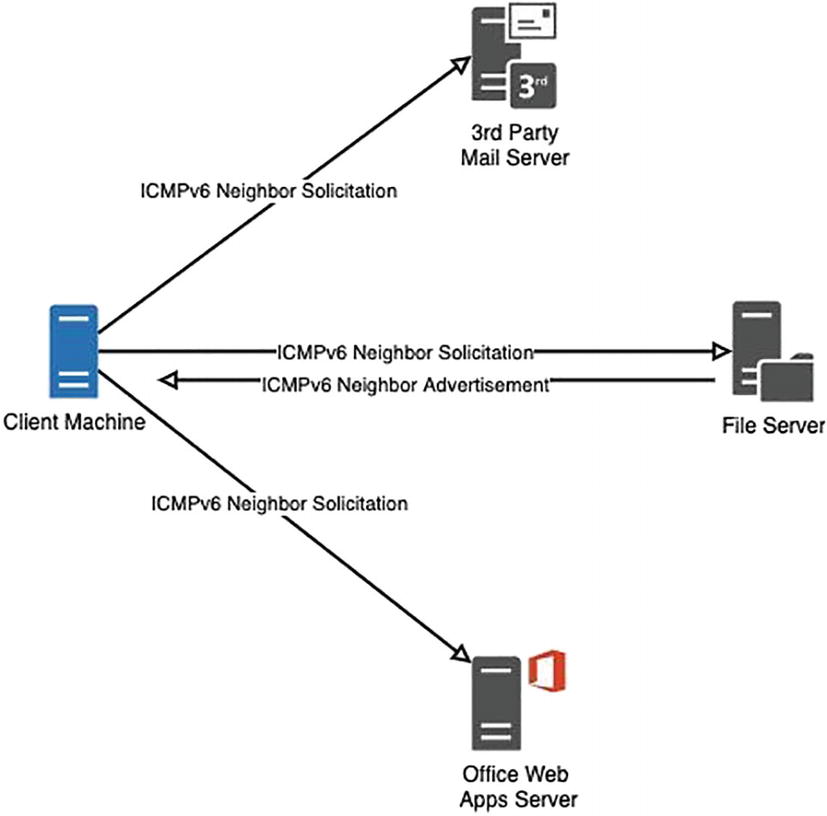
IPv6 neighbor discovery

ICMPv6 Neighbor Solicitation packet
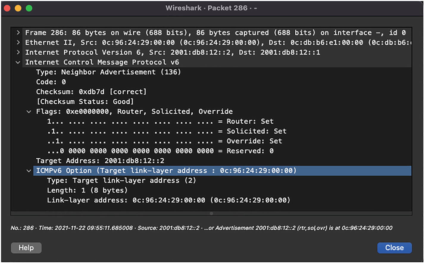
ICMPv6 Neighbor Advertisement packet
Router Solicitation (ICMPv6 Type 133): The Router Solicitation (RS) messages are sent by nodes at bootup to find a router in the local segment. These messages are sent by the hosts to the All Router Multicast Address (FF02::2). On receiving this message, an IPv6 router will generate an RA message immediately rather than waiting for the next scheduled interval. Because the destination address is a multicast address, the corresponding Layer 2 address will be in the format 33:33:xx:xx:xx:xx, where xx:xx:xx:xx:xx is the last 24 bits of the destination IPv6 address.
Router Advertisement (ICMPv6 Type 134): The RA messages are sent in response to the RS messages or periodically. The RA messages are sent to All Nodes Multicast Address. These messages consist of certain flags and options that contain the information that the interfaces on the links use to configure themselves. IPv6 routers send RA messages periodically at random intervals to reduce synchronization issues when there are multiple IPv6 routers on the segment.
Redirect (ICMPv6 Type 137): Redirects are used by IPv6 routers to inform the hosts of a better first hop for a destination.
Analyzing QoS Markings
Almost every organization utilizes time-sensitive applications such as VoIP or streaming media, routing protocols, and so on. Because the global Internet is unpredictable, there are chances that such critical and time-sensitive applications could be dropped. The traffic for such applications should be given higher priority and treated differently in the network than the usual data traffic. To do that, the IPv4 header has the Type of Service (DSCP + ECN) field and the IPv6 header has the Traffic Class field, which allow the user to set DSCP values that will categorize different application traffic. The network devices such as routers and switches can then be configured to treat the traffic based on their DSCP values.

QoS at Layer 2
Priority code point (PCP): 3-bit
Drop Eligible Indicator (DEI): 1-bit
VLAN Identifier (VID): 12-bit
The PCP field refers to the IEEE 802.1p CoS and maps to the frame priority level. The values of this field are used to prioritize different classes of traffic.
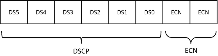
DiffServ field
Default Forwarding (DF) : Any traffic that does not meet the criteria of any of the defined classes falls under the category of Default Forwarding. The default and recommended DSCP value of this class is 0.
Expedited Forwarding (EF) : RFC 3246 defines the EF per-hop behavior (PHB) for traffic that has low delay, low loss, and low jitter requirements. This class is suitable for voice, video, and real-time service traffic. The recommended DSCP value of EF is 46.
- Assured Forwarding (AF) : RFC 2597 and RFC 3260 define the behavior for the AF class. This class assures delivery of traffic if the traffic does not exceed some subscribed rate. Within AF, four separate classes are defined and packets within each class are given drop precedence (low, medium, and high). Note that the traffic within one class has the same priority. Table 3-9 shows the different AF classes categorized based on their drop probability.Table 3-9
Assured Forwarding Classes Based on Drop Probability
Drop Probability
Class 1
Class 2
Class 3
Class 4
Low
AF11 (DSCP 10)
AF21 (DSCP 18)
AF31 (DSCP 26)
AF41 (DSCP 34)
Med
AF12 (DSCP 12)
AF22 (DSCP 20)
AF32 (DSCP 28)
AF42 (DSCP 36)
High
AF13 (DSCP 14)
AF23 (DSCP 22)
AF33 (DSCP 30)
AF43 (DSCP 38)
Class Selector: Before DiffServ, IP networks used the IP Precedence field in the ToS byte to prioritize the traffic to maintain backward compatibility with devices that still use IP Precedence, and the Class Selector PHB was defined. Table 3-10 lists all the IP Precedence values.
IP Precedence Values
Value | IP Precedence Bits | IP Precedence Name |
|---|---|---|
0 | 000 | Routine |
1 | 001 | Priority |
2 | 010 | Immediate |
3 | 011 | Flash |
4 | 100 | Flash Override |
5 | 101 | Critical |
6 | 110 | Internetwork Control |
7 | 111 | Network Control |
DSCP and IP Precedence Values
DSCP Value | Decimal Value | Meaning | IP Precedence Value |
|---|---|---|---|
101 110 | 46 | Expedited Forwarding (EF) | 101 – Critical |
000 000 | 0 | Best Effort/Default | 000 – Routine |
001 010 | 10 | AF11 | 001 – Priority |
001 100 | 12 | AF12 | |
001 110 | 14 | AF13 | |
010 010 | 18 | AF21 | 010 – Immediate |
010 100 | 20 | AF22 | |
010 110 | 22 | AF23 | |
011 010 | 26 | AF31 | 011 – Flash |
011 100 | 28 | AF32 | |
011 110 | 30 | AF33 | |
100 010 | 34 | AF41 | 100 – Flash Override |
100 100 | 36 | AF42 | |
100 110 | 38 | AF43 | |
001 000 | 8 | CS1 | 1 |
010 000 | 16 | CS2 | 2 |
011 000 | 24 | CS3 | 3 |
100 000 | 32 | CS4 | 4 |
101 000 | 40 | CS5 | 5 |
110 000 | 48 | CS6 | 6 |
111 000 | 56 | CS7 | 7 |
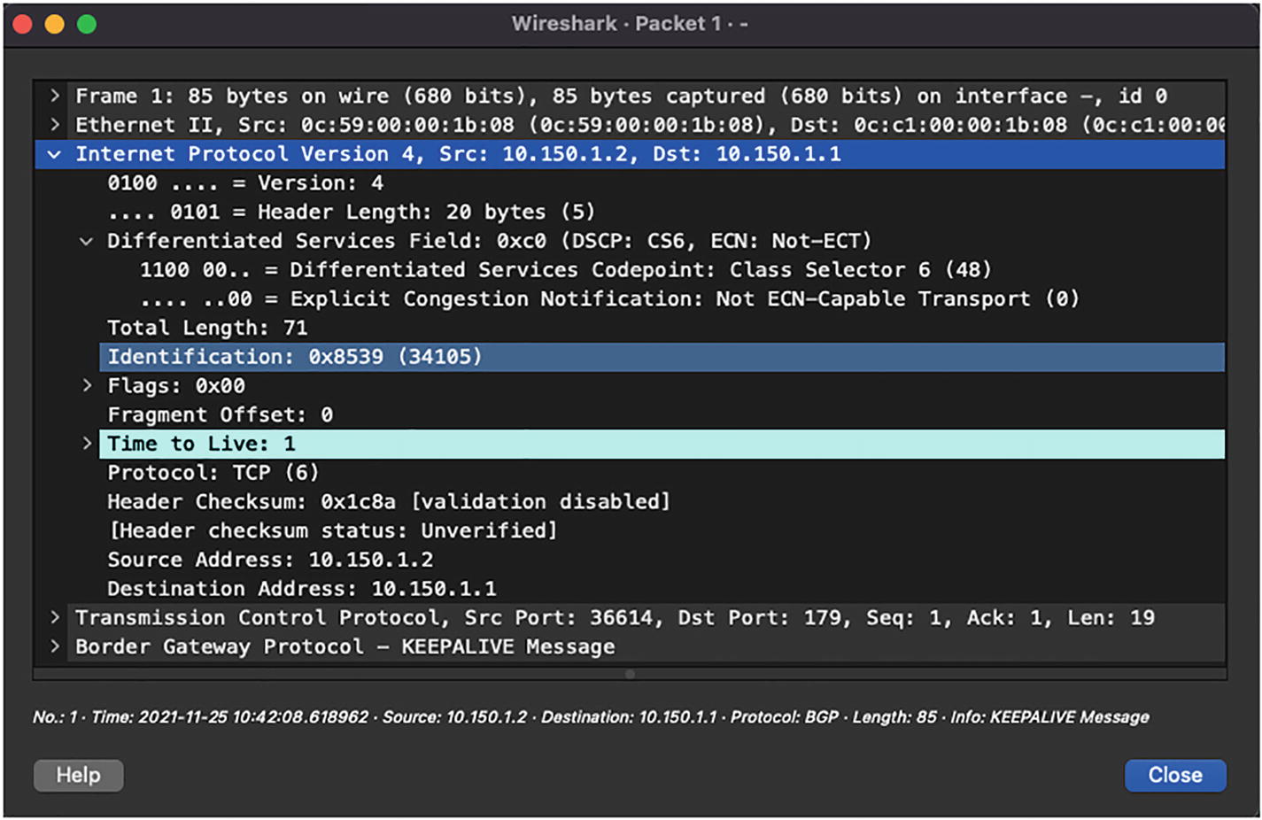
Wireshark capture of BGP packet
Using PING for Traffic Simulation with DSCP Settings
ECN bits in the DiffServ field will be covered in the next chapter.
Summary
By now, you should understand the Layer 2 and Layer 3 concepts as well as have a solid foundation about the different fields in Ethernet, IPv4, and IPv6 headers. In this chapter, we covered in detail the Layer 2 header, specifically the Ethernet header, and learned about various EtherTypes. We also learned about the IPv4 header, including how the packets get encapsulated inside the IP header and uses of various fields in the IP header. We also covered the ICMP header and how it can be used for troubleshooting purposes, and how ICMP messages can be used to notify the network about incorrect network MTU settings.
We then moved on to IPv6 headers, which helped network operators transition from 32-bit addressing to 128-bit addressing. We discovered some of the benefits of IPv6 over IPv4 headers and how they reduce the need for having broadcast packets by performing neighbor discovery using ICMPv6 headers. We learned that in IPv6, NDP leverages different ICMPv6 messages such as Router Solicitation, Router Advertisement, Neighbor Solicitation, Neighbor Advertisement, and Redirect message.
We also learned that the ICMPv6 messages are sent to different IPv6 multicast addresses. Finally, we ended this chapter learning about how QoS can be used in the network and how the DSCP values can be used to treat each type of application traffic differently.
Reference in This Chapter
RFC 1918: Address Allocation for Private Internets, by Y. Rekhter, B. Moskowitz, D. Karrenberg, G. J. de Groot, and E. Lear. https://datatracker.ietf.org/doc/html/rfc1918