Chapter 3
Optical Fibers and
Amplifiers
3.1. Optical fibers
3.1.1. General
If a transparent material has a refraction index greater than the environment, all penetrating light is trapped in this material. This is this principle jewelers use when cutting precious stones to capture the environmental light. The total reflection principle was demonstrated by an Irish physicist named John Tyndal in front of the British Royal Society in 1854. His demonstration consisted of showing that a light wave guided by a water jet was able to follow curved trajectories contrary to the thought that light could only travel in a straight line. It is this principle that is used to create illuminated water fountains in which the light seems to come from inside the water jets [WIK 09].
Glass optical fibers have been used to create lighting in special locations and to enable image transmission from inaccessible (human endoscopy) or dangerous (ionizing radiation or toxic) places.
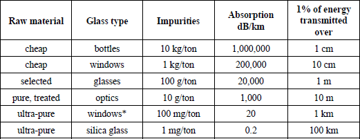
As recalled in [GOW 93], regarding telecommunications, the first optical links were laser based and the beam propagated in air (attenuation of 1 dB/km). The first to propose travel through an optical wave guide was Kao and his collaborators in 1966 [KAO 66]. At that time the attenuation in glass for visible optical wavelengths was 1,000 dB/km, due to impurities in glass. Actions were taken to reduce these impurities, leading to a reduction in the optical attenuation, both in the visible and the near infrared. This development is summarized in Table 3.1. In the last column of this table the heading indicates the length of material which is necessary to have only 1% of optical power transmitted, i.e. an attenuation of 20 dB. In fact, the attenuation values proposed by Kao to produce viable optical links were 40 dB over 2 km or 20 dB/km.
Table 3.1. Attenuation in near infrared of different glasses
*Sodium-calcium or borosilicate glass
The improvements of glass purity [GOW 93] led to an attenuation of 20 dB/km in 1970 (Corning Society); 2 dB/km in 1975; 0.5 dB/km in 1976; 0.2 dB/km in 1979 (Japanese teams, for optical wavelengths of 1.3 and 1.55 µm); and finally, the Corning Society announced 0.15 dB/km at 1.6 µm in 1982. Fibers available on the market guarantee attenuations below 0.4 dB/km at 1.3 µm and 0.25 dB/km at 1.55 µm.
It must be noted that the same process is currently being undertaken for plastic optical fibers, which went from 10,000 dB/km to 10 dB/km for a wavelength of 1 µm in a few years (Figure 3.17). In this case the improvement was achieved by modifying the material. The attenuation can still be further improved by increasing the purity of the plastic.
Apart from illumination and endoscopy, optical fibers have been developed to create temperature, pressure, bit rate, or angular velocity sensors. For example, while measuring an electric field with an aerial and a detector in an environment where an electromagnetic wave is propagating, the transfer of the magnitude measured by a copper wire considerably disturbs the field distribution. However, the information can be transported on an optical carrier in the form of an optical fiber which has no effect on the electromagnetic fields. This method is employed in electromagnetic pulses or lightning simulators, and also in test cells of radar aerials.
To see the importance of activities in optical fiber development, an edifying article proposes grouping trends from the principal authors of 4,730 publications in English between 1974 and 2007 on optical fibers [JUN 08]. In addition to this, a number of articles published in other languages must also be considered, particularly Japanese.
The use considered here is information transmission of bit rates or over distances much greater than with copper conductors or even wireless links. The collection of these applications has given rise to intense research activity and development over the past few years.
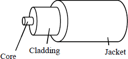
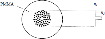
Figure 3.1 shows the general structure of an optical fiber. The core of the fiber is composed of a material that is as transparent as possible to an optical wave. The latter is surrounded by a cladding with a slightly lower refraction index to induce total reflection in the core interior. An exterior jacket ensures mechanical protection which can be reinforced to varying degrees depending on whether the fiber is in a sea bed at the mercy of the natural elements, human marine activities or sheltered in a building.
Figure 3.1. Optical fiber configuration
The optical wavelengths used for information transmission range from 0.6 to 1.6 µm. The information transmitted by optical fibers is done via pulses, solitons (particular pulses due to fiber nonlinearities), subcarriers of high frequency, or of a fixed microwave frequency modulated by pulses or diverse ultra wideband microwave signals. Pulses and solitons have been the subject of numerous articles but the systems considered in this text do not directly transmit information in the form of pulses but rather via the modulation of a fixed frequency microwave under a carrier or by varying ultra wideband modulation methods. Only the case of a high-frequency subcarrier, microwave, or ultra wideband signal modulation of the amplitude of the optical signal is considered here. For example, the effects on an optical fiber on pulse widening will not directly be considered here but will be replaced by a description of the phenomena leading to the annihilation of the microwave frequency (multi-path, multi-mode, or chromatic dispersion).
The following sections present the different aspects of the operation and performance limits of optical fibers, which are initially based on fiber cores and claddings composed of silica glass. The chapter is concluded by discussions of the replacement of glass by more cost-effective plastics for short or medium spans. The phenomena involved and discussed are the attenuation and dispersion due to the materials, total reflection, numerical aperture, the operation description of a fiber with a ray technique and then a guided modes analysis, the different fiber types, and finally, a broad outline on plastic fibers.
3.1.2. Material attenuation
Figure 3.2, which completes Figure 1.3 from the introduction, highlights the different sources of attenuation in glass optical fiber cores.
In silica (SiO2), molecule vibrational resonances occur in the ultraviolet (λ < 0.4 µm) and in the far infrared (λ > 7 µm). These resonances introduce large spectrum attenuations indicated in Figure 3.2. Silica is an amorphous material with microscopic density fluctuations. These fluctuations induce diffractions leading to losses described by Rayleigh. These losses are as such:
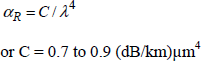
Figure 3.2 shows that Rayleigh diffraction is the principal attenuation limit between 0.6 and 1.6 µm. For λ > 1.6 µm, the limit is due to infrared absorption. Near these limits impurities, as well as the numerous metals (Fe, Cu, Co, Ni, Mn, and Cr), of which the slightest trace induces a considerable attenuation at these wavelengths, must be eliminated. As indicated in Table 3.1 the content must be lower than one part per billion.
Another component able to cause losses is hydrogen contained within water vapor. It readily propagates within the material and bonds with SiO2 to form OH radicals, with a vibrational resonance of 2.73 µm. The harmonics and combinations of SiO2 resonances give peaks at 1.39, 1.24, or 0.95 µm (see Figure 3.2).
Figure 3.2. Optical attenuation in a material
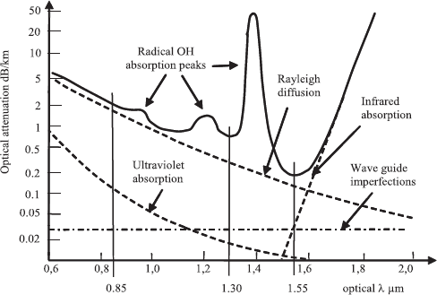
Figure 3.2 does not only show losses in bulk material, it also presents losses due to imperfections in optical guides, such as interface core/cladding, curvatures of the fiber, and random misalignments (compression of a fiber against a partition). In Figure 3.2 it is noticeable that for existing fiber production techniques and installation rules, the losses due to these imperfections remain at an acceptable level.
To summarize, at lengths of approximately 1.55 µm, a loss of 0.2 dB/km is expected, around 1.3 µm the loss is approximately 1 dB/km, and around 0.85 µm it is approximately 2 dB/km. A loss of 2 dB/km is not acceptable for a transatlantic connection but these loss values are acceptable for the connections of several hundred meters or a few kilometers considered in this text.
Numerous studies have been conducted to find a material in which the losses are lower than in silica, but other fiber requirements, such as mechanical behavior, non-toxicity, low cost, etc., mean that silica remains the most frequently used material.
For small distances, plastics can be considered. Their recent performances are of particular interest and these materials will be examined in a dedicated section.
3.1.3. Material refraction index and dispersion
The next sections present the frequency limitations for the optical transmission of a microwave signal. For this, it is necessary to start from the same notions as those presented in [GOW 93] where these ones are used to explain the bit rate limitations in an optical transmission of pulses.
A material such as silica has a refraction index varying as a function of the optical wavelength λ. The variation of this refraction index n as a function of λ is given by equation [3.2] from [GOW 93] where the numerical values comprise more significant numbers without the difference in results being significant:
[3.2] 
The corresponding curve is given in Figure 3.3.
From this curve, a chromatic dispersion index due to material Dm can be deduced. Its expression as a function of refraction index n is given below without demonstration [GOW 93]:
Figure 3.3. Refraction index of silica function of the optical wavelength
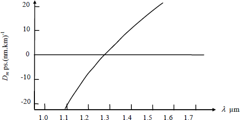
The value of Dm as function of λ is given in Figure 3.4.
Figure 3.4. Silica Dm chromatic dispersion index as a function of λ
In fibers the core is generally pure silica and the cladding must have a slightly lower refraction index. A reduction of the refraction index is obtained by doping silica with boron trioxide (B2O3) or fluorine (F). For an approximate example [GOW 93], a 1% F or 13% B2O3 doping induces a reduction of n by approximately 0.005 (n goes from 1.450 to 1.445 for λ = 1.07 µm). For other fiber configurations, an increase in n can be obtained with germanium dioxide (GeO2) of which a proportion of 13.5% increases the silica index from 1.45 to 1.47 at the same wavelength λ = 1.07 µm.
3.1.4. Total reflection, numerical aperture, transmitted maximum frequency
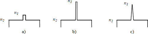
The diagram in Figure 3.5 recalls the total reflection principle. If a light ray arrives at the interface between two environments of refraction indices n1 and n2 with n1 > n2, the angles are given by the Snell-Descartes law:
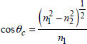
where θ1 and θ2 are the refraction angles defined in Figure 3.5a. Where θ2 = π/2, a critical angle θc appears such that:
and for θ1 > θc, total internal reflection occurs.
From this law, the first step is to describe the injection of light in a fiber and its propagation within by a radiation method. This method is a summary but indicates the problems that need to be resolved.
Figure 3.5. Reflection at interface n1/n2: a) refraction; b) critical angle; c)total reflection
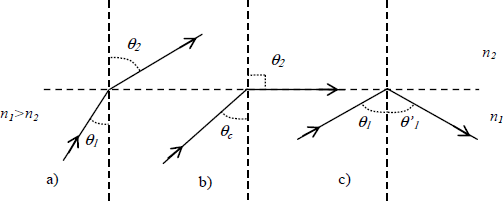
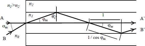
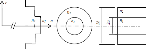
Figure 3.6 shows a cylindrical optical fiber vertical cross-section as in Figure 3.1.
The refraction indices of the core and cladding are n1 and n2 and the exterior index is n0. The maximum entry angle αm gives a reflection angle at interface n1/n2 superior or equal to θc and so an angle φm = π/2− θc. The Snell-Descartes law hence gives the value of αm:
[3.6] ![]()
Taking into account [3.6]:
where:
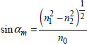
Figure 3.6. Rays in an optical fiber
This expression allows the definition of the numerical aperture (NA) of a fiber:
with:
![]()
If a diffuse light source is now presented in front of the fiber as shown in Figure 3.7, the intensity of light depends on angle φ by expression I0 cosφ.
If this source is presented to a fiber, the light power proportion entering the fiber is given without proof [GOW 93]:
and
[3.11] ![]()
Figure 3.7. Diffuse light sources
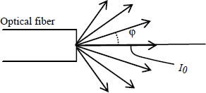
The reduction of losses due to coupling between light sources and an optical fiber and between this fiber and a photodetector remains one of the principal problems to resolve in photonic systems. From expression [3.11], the fiber index must be as high as possible and the index difference with the core must be large. A good solution is to use fibers without cladding to maximize Δn, but two reasons prevent this solution.
The ray method does not account for the fact that at the interface n1/n2 reflection point an evanescent wave propagates in environment n2. The presence of a cladding is hence indispensable to confine this evanescent wave and hence reduce losses resulting from it.
Elsewhere, as shown in Figure 3.6, the rays entering the fiber (AA’ or BB’) can follow paths of different lengths. Usual optical communications being done by pulses, these multi-paths result in a broadening of the pulse. In the case of high-frequency wave transport considered in this work, these multi-paths can instead lead to the cancellation of the microwave subcarrier. To increase the extinction frequency, Δn must be reduced. This will now be examined.
Section 6.1.3 details the expressions describing the propagation of an optical signal modulated by a microwave frequency in an optical fiber.
Equation [3.12] gives the electric field ![]() after travelling a length L:
after travelling a length L:
[3.12] 
with:
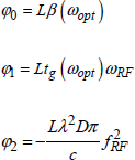
where fRF is the microwave frequency corresponding to the angular frequency ωRF and ωopt is the optical angular frequency.
After photodetection the current is given by equation [3.14]:
In this expression only the term ωRF is taken into account and the chromatic dispersion is negligible, so the most important term after photodetection is:
[3.14] ![]()
If the phase difference between the two photodetected signals after path AA’ and path BB’ is equal to π, these signals will cancel.
From the definition of φ1 this can be written:
and by putting:
![]()
and by considering the velocity of group vg ≈ v p where vp is phase velocity, the RF frequency that cancels signals from the two paths is:
[3.16] ![]()
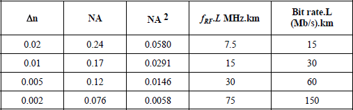
Table 3.2 gives some corresponding maximum frequency and numerical aperture values, which clearly demonstrate that the higher the transmitted frequency the lower the numerical aperture.
The first three and the last columns are from [GOW 93].
NOTE:- The fourth column gives the maximum frequency in terms of expression [3.16], whereas the fourth column gives the maximum bit rate, which is the number normally given when the broadening of transmitted pulses is considered. The values in megahertz per kilometer of Table 3.2 correspond to half of the maximum bit rate values expressed in megabits per second kilometer usually given. It shall be seen further on that the frequency values noted above are pessimistic.
Table 3.2. Maximum admissible frequency from high-frequency subcarriers accounting for multi-paths of 1 km of a step-index fiber
3.1.5. Step-index fiber
The example fibers in the previous section are step-index fibers. The diagram of this fiber type is presented in Figure 3.8.
Figure 3.8. Step-index fiber
The first fibers were of this type. The analysis undertaken in the previous section from a ray method is rough, and the values of Table 3.2 have to be specified. It is nevertheless true that the step-index fiber is inconvenient for microwave frequency transmissions even over distances of a few hundred meters.
Instead of an analysis by rays, a modal analysis as done in the appendix, section 3.3, can be performed. It is hence possible to establish curves representing the modes appearing in the fiber as a function of a normalized optical frequency V given by expression [3.17]:
[3.17] ![]()
where v is the optical frequency.
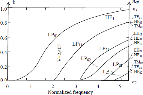
The curves of Figure 3.9 show the first LP (linear polarization, see appendix, section 3.3) modes, which appear in a step-index fiber as a function of the normalized optical frequency recalled above. These fibers are multimode as are the graded index fibers of next section.
In this figure the ordinate value b is given in the appendix by equation [3.49]. This representation allows modes to be plotted on a universal diagram independent of the values of n1 and n2. These values can however be placed on the right ordinate as in Figure 3.9.
Figure 3.9. LP (linearly polarized) modes in a step-index fiber
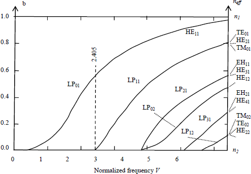
Given a step-index fiber for which n1 = 1.442, 2a = 100 µm, Δn = 0.01, operating at λ = 1.5 µm. In this case V = 35. As the curves in Figure 3.3 do not go above V = 6, it is apparent that for V = 35, the number of modes is high. It will be possible to consider that extreme modes will essentially have refraction indices of n1 = 1,442 and n2 = 1,431.
Extreme modes propagate with an index n1 and n2, two different paths can be introduced and hence two different φ1 values in equation [3.14]. By making the same approximations (for vg≈ vp it is sufficient to not be too close to the mode cutoff frequency), the value of fRF, which cancels these two signals, is also given by equation [3.16]. However, in this case it has been shown that these two values correspond to extreme modes (the fastest and slowest), whereas dozens of other different modes can propagate. The extinction is hence not as abrupt as the ray calculation suggests. The transportable microwave frequency values shown in Table 3.2 are hence fairly pessimistic. Measurements on step-index guides should be done to confirm this observation. The fact remains that acceptable modulation frequencies for 1 km of a step-index fiber remains very low.
It must be noted that the evanescence phenomenon due to different propagation velocities according to multimode fibers takes place even for a unique frequency, and has no connection with evanescence of a double sideband microwave modulation seen for single-mode fibers.
3.1.6. Graded index fiber
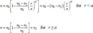
In graded index fibers the refraction index at the fiber core shows a progressive reduction from the center to radius a; this is shown in Figure 3.10.
Figure 3.10. Graded index fiber
Refraction index n(r) is written:
In these expressions parameter α has great importance. It will be seen later that this parameter is different for glass and plastic fibers.
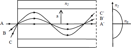
Figure 3.11 shows three light rays AA’, BB’, and CC’ propagating in such a fiber with start point r0 and direction ![]() Provided the path stays within proximity of the fiber axis (low r0), the equation describing the path is given by expression [AGR 92; GOW 93]:
Provided the path stays within proximity of the fiber axis (low r0), the equation describing the path is given by expression [AGR 92; GOW 93]:
For r < a and α= 2, the general solution to this equation is:
[3.20] ![]()
with:
Equation [3.20] shows that whatever the path taken, the rays cross for z = 2 mπ / p. Hence there is no intermodal dispersion. This expression is only valid for rays close to the axis.
Figure 3.11. Light rays in a graded index fiber
For a real fiber the accepted expression is a little different:
[3.21] 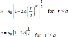
with:
![]()
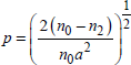
For value α, its optimum is:
The optimal α value is extremely precise, showing the difficulty in realizing such a fiber. This is shown in Figure 3.12, which describes the hoped intermodal dispersion of a graded index fiber recalled in [AGR 92].
Certain authors have described the modal analysis of this fiber type [BEL 99; GOW 93]. The expressions obtained are slightly more complex than those concerning step-index fibers and are outside the scope of this work.
Figure 3.12. Intermodal dispersion as a function of α in a graded index guide
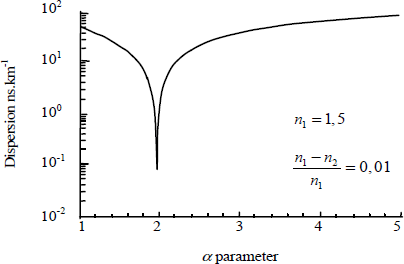
In a graded index fiber the intermodal dispersion can be improved by three orders of magnitude [AGR 92] in comparison to a step-index fiber. In comparison with Table 3.2, it is hence possible to obtain a bandwidth of approximately 5 GHz.km. For this reason most currently available multimode fibers are graded index fibers.
3.1.7. Single-mode fiber
Figure 3.9 showed that for an optical fiber a fundamental propagation mode exists: mode LP01 or HE11, which propagates down to a frequency of 0. Between frequency 0 and the frequency where mode LP11 appears, the propagation in the optical fiber on mode LP01 is single-mode. The use of single-mode fibers completely eliminates intermodal dispersion. Referring to Figure 3.9, it appears that providing V < 2.405, the propagation in a step-index fiber is single-mode. From the definition of V (equation [3.92]), this is obtained by altering a and the index gap between the core and the cladding. The standard single-mode fiber (referenced G652 according to the nomenclature of the International Telegraph and Telephone Consultative Committee) has a core diameter of 8.7 μm. The core index (pure silicon) is 1.514 and the cladding index (silicon doped with fluorine) is 1.4473 at 1,300 nm. In these conditions, V=2.292, which corresponds to a normalized frequency lower than than that of the appearance of the second mode.
However, for a core diameter that is also low, the electric fields overflow into the cladding. The particular field form must be accounted for to recalculate the new waveguide cutoff wavelength [GOW 93]. Once the analysis is performed the second mode still does not appear.
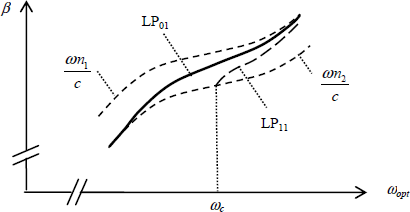
Now, intramodal or chromatic dispersion phenomenon becomes dominant. This dispersion is composed of a dispersion due to the material studied in section 3.1.3 and a dispersion due to the fact that the optical fiber is an optical guide; this is demonstrated in Figure 3.9. The combination of these two dispersions is represented on the curve in Figure 3.13 representing the propagation constant, β, as a function of angular frequency ωopt. On this figure the fundamental mode, LP01, and the first superior mode, LP11, appear (cutoff angular frequency ωc).
Figure 3.13. Propagation constant,β as a function of angular frequency,ωopt, in an optical fiber
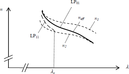
This curve can also be represented in the form of different variations of refraction indices as a function of optical wavelength, λ, as demonstrated in Figure 3.14.
From these curves the chromatic dispersions can be extracted. From the curve in Figure 3.14, the chromatic dispersion is established in section 6.1.2 and is given by equation [6.8]:
From the curves in Figure 3.14, the same chromatic dispersion is given by equation [3.24]:
[3.24] ![]()
Figure 3.14. Refraction indices as a function of optical wavelength in a multimode fiber
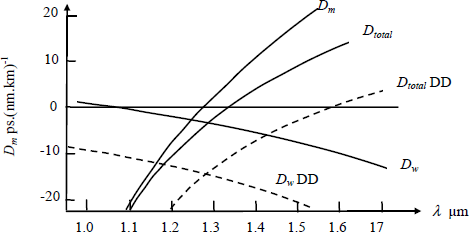
With these expressions it is hence possible to extract the chromatic dispersion due to the material (Dm) and the dispersion due to the unique mode (in the zone where only the LP01 mode exists) in a fiber (Dw), and finally, the total dispersion, which is the sum of these two dispersions. The corresponding values are presented in Figure 3.15 [GOW 93].
For normal fibers (solid lines in the figure), 0 dispersion appears around 1.3 µm. It is possible to obtain a dispersion of 0 shifted towards larger wavelengths by modifying the fiber doping profiles [GOW 93]. Figure 3.16 represents the normal doping profile (a) and two profile examples to obtain a shift of 0 dispersion (b and c).
To summarize, in single-mode fibers intermodal dispersion is eradicated but an intramodal dispersion appears with the effect of microwave modulation evanescence in the case of double sideband modulation. These effects are discussed in section 6.1. First, this occurs for modulation frequencies much higher than for graded index fibers (evanescence for a 9 km standard fiber is 20 GHz at 1.5 µm), but also there is an optical wavelength for which this dispersion is practically 0 (approximately 1.3 µm for standard single-mode fibers). It is also possible to shift this 0 dispersion frequency towards a wavelength of 1.5 or 1.6 µm. It will be seen in section 6.1 that if it is possible to perform a single sideband microwave modulation, this evanescence disappears. It should be noted that for small fiber lengths the modulation frequencies can increase, but at 60 GHz the fiber cannot be longer than 100 m [WEI 08].
Figure 3.15. Chromatic dispersions in standard single-mode optical fibers (solid lines) and at shifted dispersion (dotted lines=SD)
The previous remarks are valid only for optical wavelengths of 1.3 to 1.6 µm. For wavelengths of 0.8 µm, the value of a (radius from the fiber core) must become very small and the realization of single-mode fibers becomes problematic. Also, the realization of connectors is even more difficult and costly in this case.
Figure 3.16. a) Doping profile for a normal single-mode fiber; b) and c) at shifted dispersion
3.1.8. Plastic optical fibers
3.1.8.1. Introduction
Plastic optical fibers are in full development. At least for short links, different materials have been revealed in the last few years that have losses and prices that are sufficiently low for them to replace silica-based fibers. As the links examined in this work are generally short (10 m to 1 km), it is necessary to review this fiber type. The plastic materials currently studied are PMMA and other polymer forms where the PMMA hydrogen atoms are partially or completely replaced by deuterium or fluorine.
Attenuation of the materials is the first characteristic to be described. Then we will examine how dispersion develops as a function of wavelength in comparison to silica. The three fiber types described in the previous sections led to plastic fiber realizations. Step-index, gradient index, and single-mode fibers are presented. This section will finish with a discussion of the future developments of this fiber type.
3.1.8.2. Attenuation of plastic optical fibers
The base material is PMMA, which is well known under the names “Plexiglas” or “Altuglas”. It has hydrocarbon chains that cause optical absorption peaks due to molecular resonance and their harmonics. If the hydrogen atoms are replaced by deuterium (perdeuterium-PMMA), the optical attenuation is reduced, this attenuation is further reduced if the hydrogen atoms are replaced by fluorine atoms to create fluorinated PMMA. If this fluorination is partial the cost of the material is reduced and the reduced attenuation is also only partial but this can be sufficient.
The curves of Figure 3.17 show the attenuation of these different materials [KOI 06; KOI 09]. These values are evaluated on graded index fibers, but these curves show the trends for different materials as well.
The curves of Figure 3.17 demonstrate the attenuation of PMMA, which show an attenuation window at the origin in the visible range, around 650 nm. However, these curves also show the surprising improvement achieved by replacing the hydrogen by deuterium or fluorine.
Figure 3.17. Attenuation measured for materials in plastic optical fibers from graded index fibers [KOI 06; KOI 09]
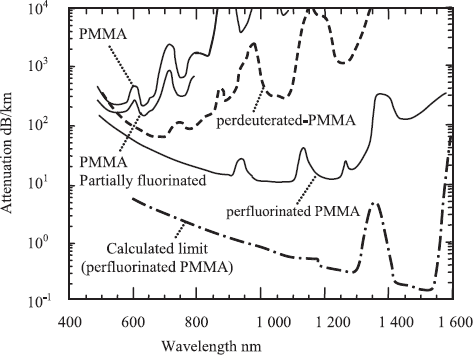
Attenuations of a dozen decibels per kilometer can be considered around 1,200 nm. Regarding theoretical calculations, an improvement on this value is theoretically possible, which will enable the use of plastic fibers over long distances.
3.1.8.3. Plastic optical fiber dispersion
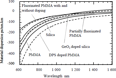
The dispersion of different materials is shown in Figure 3.18. It can be observed that the dispersion variations are less for materials such as PMMA than for silica. It should also be noted that PMMA doping (diphenyl sulfide doping (DPS)) changes the dispersion, whereas this is less the case for silica GeO2 doping and even less for the doping of fluorinated PMMA.
This has consequences that will be discussed in the section on graded index optical fibers.
Figure 3.18. Dispersion for materials in plastic optical fibers from graded index fibers [KOI 06;KOI 09]
3.1.8.4. Step-index plastic fibers
The first plastic fibers were step-index fibers [BRU 02]. The diameter of the core was in the order of millimeters and the number of modes was considerable: in the order of 50,000 [KOI 06]. This led to a considerable intermodal dispersion and hence to a pulse bit rate in the order of 50 Mb/s over 100 m. The material used was PMMA, the wavelength used was 650 nm, which corresponds to an attenuation of 150 dB/km. The only use foreseen was the transmission of data between different car components where the copper cable replacement by a plastic material offered many benefits (cost, electromagnetic compatibility, and weight).
The step-index core was first replaced by multilayered core fibers, composed of concentric layers with different indices. Then appeared with cores composed of a bundle of 12 very fine fibers. These two types allowed bit rates of 500 Mb/s over 50 m of fiber [KOI 06].
NOTE.- For the comparison between bit rates mentioned above and the maximum frequency of a microwave carrier, see Table 3.2.
3.1.8.5. Graded index plastic fibers
The following stage was the development of graded index fibers. The graded index is realized by doping PMMA with benzyl benzoate or diphenyl sulfide. The graded index model is given by equation [3.21] shown in section 3.1.6 for silica fibers. For the latter, the α parameter optimum (slightly lower than 2) was obtained by only considering the propagation in the optical wave guide. For plastic fibers, the optimum was researched by also accounting for the chromatic dispersion of the material. Here the α optimum is slightly different. It is situated around 2.3 for benzyl benzoate PMMA doping, 2.42 for diphenyl sulfide PMMA doping, and 2.1 for fluorinated PMMA [KOI 06].
Fluorinated graded index fibers allow bit rates of 10 Gb/s for 100 m of fiber at a wavelength of 850 nm to be obtained. It is with these fibers that an advantage of fluorinated PMMA appears; the refraction index variation with the wavelength is smaller than that of silica. Thus a profile optimized for 850 nm remains optimized for 650 nm, this is not the case for silica (see the dispersion curves of silica and fluorinated PMMA on Figure 3.18 [KOI 06]).
3.1.8.6. Single-mode plastic fibers
To obtain single-mode fibers, the fiber core dimensions must be reduced. This dimension must be further reduced for an optical wavelength of 650 nm than for a wavelength of 1,300 nm as in silica. This was obtained by surrounding the fiber core with a photonic crystal structure [BRU 02; KOI 06] as shown in Figure 3.19. This structure is obtained by making air tubes in the structure, around the core. The material around the core is composed of a material with a lower refraction index, introducing a guidance around the very small core.
Figure 3.19. Microstructure diagram of a photonic crystal based a single-mode plastic fiber composed of holes in the PMMA [BRU 02]
This structure was not extensively developed as the very restrained dimensions of the core forced a return to very tight tolerances and hence to very high costs for the connection structures of these fibers.
3.1.8.7. Summary
Plastic optical fibers have the advantages of being made from a cheap material and their dimensions are larger than glass fibers (1 mm diameter). This allows low-cost fiber manipulation, be it for cutting or equipping it with cheap connectors. These fibers were first used in data transmission in cars where replacing copper wires is very advantageous. Radical loss reductions obtained using fluorinated PMMA then enabled these fibers to be used in local information distribution networks (high bit rate information in universities and very high bit rate information, such as complex images in hospitals) with the help of graded index fibers, even if this meant reducing the diameters of the fibers. The possible bit rates achieved with this type of fiber (10 Gb/s for 100 m) make it a very good candidate for microwave transporting networks. Especially as the loss calculations show that further improvement can still be achieved.
Although single-mode plastic fibers are available, the very restraining core dimensions increase connector costs meaning they have not emerged onto the market yet.
3.2. Optical amplifiers
The first optical communications systems used multimode optical fibers and they showed the benefit of amplifying the optical signal to enable communication over long distances, by refraining from using optoelectronic repeaters, which limit the electric signal frequency [JOI 96].
This is the same for single-mode optical fibers, which weakly attenuate the electric signal but destroy it due to chromatic dispersion.
Direct optical amplification is hence a beneficial procedure for long-distance communications, such as intercity and marine communications. However, signal amplification can also be a valuable contribution in a microwave photonic link assessment.
There are two types of optical amplifiers:
– the semiconductor optical amplifier or SOA appeared in the early 1980s and was very sensitive to optical signal polarization. This sensitivity was greatly reduced and can be used in the spectral window of 1,300 nm, for very high bit rate applications and for other applications due to their multifunctional properties (detection, modulation, frequency transposition, etc.);
– erbium fiber-doped amplifiers (EFDAs) appeared in the late 1980s and are largely used in long-distance communication in the 1,550 nm spectral band [SAI 92].
Optical signal amplification relies on the stimulated emission phenomenon: the signal propagates in an adequately doped optical guide on which an external source is applied (current source or injected light named pump), which creates a population inversion in the dopant. The stimulated emission photons coherently add themselves to the propagating photons constituting the optical signal, which is then amplified. At the same time, photons linked to spontaneous emission are emitted, which constitute non-coherent noise inherent to the optical amplifier.
Optical amplifiers will thus develop similar characteristics to those met in an electronic amplifier, namely the gain saturation, noise, and nonlinearities, of which the results of an optical link must be accounted for.
However, optical amplifiers have one aspect that differentiates them from electronic amplifiers: they amplify from the input to output but also vice versa. This aspect means special precautions must be taken when introducing them into an optical link, regarding reflection reduction during interconnections and gain partitioning in optical parts.
3.2.1. Semiconductor optical amplifiers: SOA
This type of component has an identical structure to a Fabry-Perot and multiple quantum well diode laser except there are no reflective mirrors at the cavity ends to avoid the resonant effect while amplifying the signal. The pumping is electric and non-optical, which presents a great advantage for use in optical links [CON 02].
These amplifiers are realized from heterostructures of III-V materials with direct gaps (GaAs/GaAlAs, GaInAs/InP, GaInAsP/InP, and InAlGaAs/InP). Thus wavelengths of 850 and 1,600 nm are covered by these amplifiers, which show a gain of around 30 dB. With small dimensions they operate with an electric command and can be integrated to a diode laser or a modulator. However, they show weaker performances than EDFA amplifiers, namely a higher noise, weaker gain, weaker power, and higher nonlinearities, which distort the signal in optical communications. Thus they are considered for optical signal treatment, wavelength conversion, detection, and demultiplexing applications [UDV 08].
The vertical-cavity semiconductor optical amplifier (VCSOA) has a structure practically identical to a VCSEL, but the mirror has a weak reflection. This component has a weak gain, which can be increased by the use of a resonant cavity but reduces the bandwidth. Thus a VCSOA can be considered as a signal amplifying optical filter and can be used as a switch for wavelengths [HUR 07].
3.2.2. EDFAs
This type of optical amplifier uses a doped fiber (DFA or doped fiber amplifier). The amplified optical signal is multiplexed to that from a laser, which is used as a pump, and enters the doped fiber. The signal is amplified due to its interaction with the doping ions of the fiber.
The most frequently used dopants are erbium ions introduced into the fiber core. If the pump laser has a wavelength of 980 or 1,480 nm, the doped fiber has a gain around 1,550 nm. As a result the photons emitted by the pump laser are absorbed by the doping ions allowing the free electrons to attain a superior energy level. They return to a lower energy level by emitting a photon through stimulated emission at longer wavelengths than those of pump lasers. In this process certain photons are emitted by spontaneous emission and others correspond to phonon originating non-irradiative emission, hence contributing to the reduction in amplifier gain.
This amplifier type has a gain spectrum composed of several wavelength peaks, which is linked to the previous mechanisms and to the different existing energy levels in erbium ions. It is hence a relatively wide optical bandwidth (around 30 nm). Thus it is useful in communication systems multiplexed in wavelengths (WDM = wavelength division multiplexing) as a single amplifier is used to amplify several optical signals present in the optical fiber, which transport different information.
The principal noise source from doped fiber optical amplifiers is the amplification of spontaneous emission (ASE = amplified spontaneous emission), corresponding to a spectral response close to that of the gain. As a result, the electrons present in the high energy levels descend from these levels by spontaneous emission. These photons are hence emitted in all directions of the fiber, including the propagation direction of the optical signals. By interacting with the dopants in the fiber, the photons are also at the origin of new spontaneous emissions, which over the course of their trajectory participate in the amplification of this spontaneous emission. This generated signal induces a degradation of the optical signal containing the information as it propagates along the link and is detected by the receiver in the same fashion as the optical signal. It contributes to system performance degradation by introducing a noise factor, which varies between 6 and 8 dB, but it equally reduces the optical amplifier gain.
The gain in such a structure is introduced by a population inversion of the doping ions. The gain saturation appears when the optical signal power increases or when the pump signal is reduced, then the inversion level and gain is reduced. However DFA show a noise optimum if operating in a saturation zone, typically for a gain compression of 10 dB.
We define the polarization gain (DPG = gain-dependent polarization) introduced by a change in the gain value according to the alignment of the polarization of the optical signals that require amplification and the signal from the pump laser. This phenomenon is difficult to observe on one DFA with a length of many meters. However, it cannot pass unnoticed in links using several amplifiers one after the other.
The most used amplifier is the EDFA [DES 87; MEA 87] as the amplification is in the third window of a silica fiber spectral transmission (Figure 3.2). This amplifier operates at the two optical spectrum bands used in optical communications: C-band (conventional band) from 1,525 to 1,565 nm and L-band (long band) from 1,570 to 1,610 nm. The gain is adapted according to the band used by varying the length of the doped fiber, shorter lengths for C-band than for L-band. The pump laser can emit at 980 nm; in this case low noise performances are better. It can also emit at 1,480 nm for which power performances are better. A combination of these two wavelengths is generally used for commercial amplifiers.
Other dopants are used for different wavelengths:
– in S-band (1,460 to 1,490 nm) thulium to realize “TDFAs”;
– around 1,300 nm praseodymium to realize “PDFAs”, which have lower performances than EDFAs;
– around 1 μm, neodymium or ytterbium to create “YDFAs”, which allow high powers (a few kilowatts) when coupled to a laser.
Table 3.3 shows comparisons of typical characteristics of commercialized optical amplifiers.
Table 3.3. Characteristic comparisons between 1550 nm optical amplifiers
| SOA | EDFA | |
| Gain (dB) | 13 to 28 | 30 to 50 |
| NF (dB) | 6 to 9 | 3.8 to 6 |
| Output compression@3 dB (dBm) | 9 to 18 | 13 to 33 |
| 3 dB optical bandwidth (nm) | 60 to 100 |
3.3. Appendix: modal analysis of propagation in a fiber
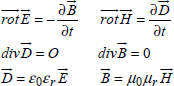
3.3.1. Maxwell equations
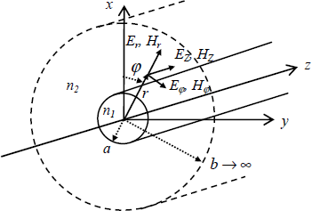
This overview regarding the analysis of electromagnetic propagation in an optical fiber is based on publications from [AGR 92; GOW 93; BEL 99; HIN 06]. Figure 3.20 represents the fiber considered. The propagation of an electromagnetic wave in a given space is defined by Maxwell equations, which in Cartesian coordinates can be written:
with:
![]()
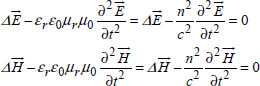
The propagation equations for electric and magnetic fields can be written:
3.3.2. Maxwell equations in a cylindrical fiber
These expressions can be rewritten in cylindrical coordinates (see Figure 3.20) with ![]() and
and ![]() . In particular, the fields on the z axis are given by the expression below with: ψz = Ez or Hz:
. In particular, the fields on the z axis are given by the expression below with: ψz = Ez or Hz:
[3.27] ![]()
When n is a constant on the z axis, on this axis the solutions are:
As r and φ functions are separated it is possible to use a modal expansion in the φ axis:
[3.29] ![]()
By introducing [3.29] in [3.27]:
The general solution to this differential is:
[3.31] ![]()
with:
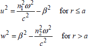
Figure 3.20. Electric and magnetic field in cylindrical coordinates r,φ, z
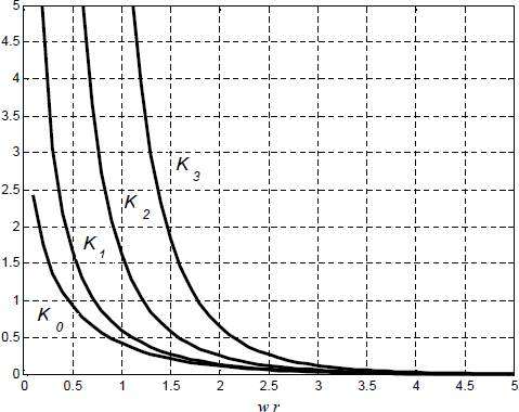
In equation [3.31], Jk and Yk are first and second-type Bessel functions, whereas Kk and Ik are first and second-type modified Bessel functions. The application of a first limit condition (ψz defined for r = 0) leads to ![]() because r = 0, Y k (ur) → ∞, and the application of a second limit condition (ψz= 0 for r → ∞) leads to
because r = 0, Y k (ur) → ∞, and the application of a second limit condition (ψz= 0 for r → ∞) leads to ![]() because r = ∞, Ik(wr)→ ∞.
because r = ∞, Ik(wr)→ ∞.
Figure 3.21 shows the first-type Bessel functions for k = 0, 1, 2, and 3.
Figure 3.21. First-type Bessel functions for k = 0, 1, 2, and 3
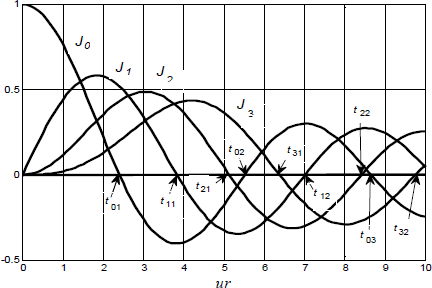
Table 3.4 shows the square roots of the first-type Bessel function from Figure 3.21.
Table 3.4. Square roots of first-type Bessel functions for k = 0, 1, 2 and 3
Figure 3.22 shows the second-type modified Bessel functions for k = 0, 1, 2, and 3.
By accounting for the expressions between fields E and H, fields Ez (r, φ) and Hz (r, φ) can now be written:
Figure 3.22. Second-type modified Bessel functions for k = 0, 1, 2, and 3
The transverse field components can be written as a function of the z components:
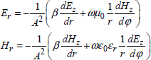
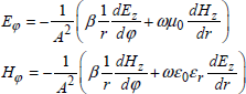
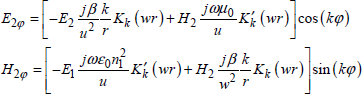
Only the transverse fields in φ will be used. For r < a (zone n1) they can be written:
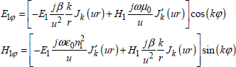
For r > a (zone n2) they become:
3.3.3. Continuity and characteristic equation conditions
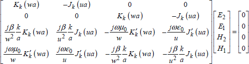
Tangent components continuity conditions for r = a can now be written in the manner below:
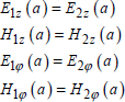
By introducing the values above, these expressions take the form of an equation system represented below:
The solutions of this system are the roots of the characteristic equation given by the equation:
[3.40] 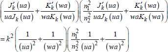
This equation is a transcendent equation whose solutions are found by numerical methods illustrated below.
3.3.4. Research of different propagation modes
A reduced frequency V is defined such that:
[3.41] ![]()
or:
This definition provides equations that are independent from the fiber core diameter (a), of the optical wavelength (λ), and the n1 and n2 values. Equation [3.41] also establishes a relation between u and w. So if a value is chosen for V the u values, which will be solutions of equation [3.40], will correspond to different electromagnetic propagation modes in the fiber.
The propagation modes can be ordered into different categories:
– for one part the “transverse” mode types. For these modes, the electric or magnetic field on the z axis is zero. If the electric field, Ez, is zero, the electric fields of this mode are only transverse, hence the mode name TE (transverse electric). If the magnetic field Hz is zero, only the magnetic field is transverse, hence the mode TM (transverse magnetic);
– other modes have fields along the z axis that are both electric and magnetic. These are hybrid modes. Certain modes have an electric field, Ez, that is much higher than the magnetic field, Hz; these are EH modes, whereas for others Hz > Ez, these are HE modes.
For example, the process taken to obtain TE modes will be described. TE and TM are obtained by making k = 0 in equation [3.40]. So this expression can be written:
[3.43] ![]()
For this expression to be exact, it is sufficient to write that one of the terms in brackets is equal to zero. The first term gives TE modes and the second gives TM modes. The first term shall be chosen (TE modes), the Bessel functions recurrence equations [ABR 72], which allow the equations of the derivatives below to be written, must be taken into account:
By taking into account equation [3.41], the equation that requires resolution is:
[3.45] 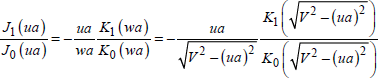
Figure 3.23 shows the graphical representation of the left term in equation [3.45], f1 and the right term f2 for three values of V.
Figure 3.23. Graphical representation of equation [3.45] for three values of V
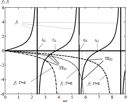
Figure 3.23 assumes the following statements:
– for each mode and V value, the intersection functions f1 and f2 give a ua value, which then allows β or neff = β/k0 to be plotted as a function of V;
– for the TE01 mode, three intersection points appear. There is also a value inferior to V below which there is no intersection. This value is given by t01 (see Table 3.4). This corresponds to the cutoff of the TE01 mode, which occurs when V = 2.405. When V → ∞, the limit value of ua is given by t11 (3.832);
– for mode TE02, there are only two intersection points. The cutoff occurs when V = t02 and the maximum ua value is given by t12.
Modes TM0m can be obtained with a similar method by considering the second term in brackets of equation [3.43]. It should be noted that ratio ![]() is very close to 1 and so the results will be very similar.
is very close to 1 and so the results will be very similar.
To obtain hybrid modes it is possible to return to equation [3.40] where:
[3.46] 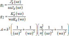
Equation [3.40] is hence written:
[3.47] ![]()
This equation can be considered as a g1 second-degree equation containing solutions written:
[3.48] 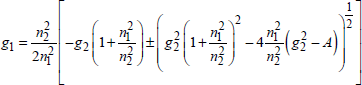
The first of these solutions (+ sign) corresponds to HEkm modes, whereas the second corresponds to EHkm modes. In these two cases, this expression can still be solved graphically by plotting the left and right terms of equation [3.48].
Figure 3.24 shows the plot of modes for V values from 0 to 10. A first solution would show index neff obtained by the steps above as a function of V. A more general solution consists of showing the axes in the form of a reduced variable or normalized propagation constant:
[3.49] ![]()
Figure 3.24. Different modes in an optical fiber with reduced ordinate
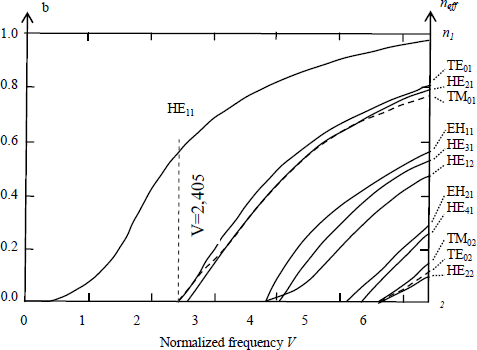
From the plot it can be seen that with axis b this figure no longer depends on n1 and n2 values. But these values can be inserted on the right axis to give an idea of mode evolution, especially if the gap between n1 and n2 is very low.
3.3.5. Approximation of linearly polarized modes
If the difference between n1 and n2 is very low another approximation can be made. It can be written:
[3.50] ![]()
By introducing this relation into [3.46] and [3.47], several of the identified modes in the previous section regroup as several degenerated forms of the same mode referred to as “linearly polarized” or the LP (linear polarization) mode.
Concerning transverse modes (equation [3.43]), there is now no difference between the propagation constants of TE and TM modes.
For hybrid modes, by inserting equation [3.50] into [3.48] and by reintroducing values g1, g2, and A, the equation becomes simplified and is written:
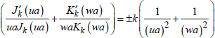
In this expression, the “+” sign corresponds to EHkm modes, whereas the “−” corresponds to HEkm modes.
Recurrence Bessel function equations are written [ABR 72]:
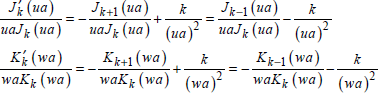
In these conditions, the expression giving HEkM, modes (minus sign) for k = 1 gives the expression:
[3.53] ![]()
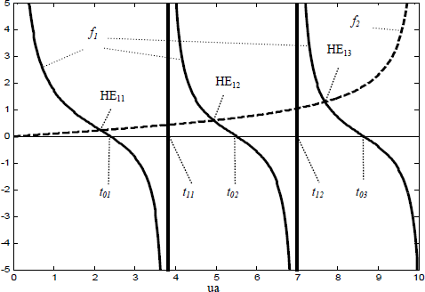
These two functions (f1 for the left term and f2 for the right term) are plotted in Figure 3.25 by introducing the relation between ua and wa as in equation [3.45]. The right term in equation [3.53] is plotted for V = 10. In view of these plots, the following comments can be made.
As shown in Figure 3.24, it is confirmed that there exists a mode (mode H11) that has a cutoff frequency equal to zero. It is the great difference with metallic cylindrical wave guides and makes one of the main advantages of optical fibers, as between V = 0 and V = 2,405 a single mode will propagate (see also Figure 3.26). Hence there is a possibility of having single-mode optical fibers.
For the two other modes appearing in this figure it is possible to define a cutoff (normalized) frequency (t11 for HE12 and t12 for HE13) and a maximum ua value (t02 for HE12 and t03 for HE13).
Figure 3.25. Graphical representation of equation [3.53] for V = 10
It is now possible to transform Figure 3.24 by showing only the LP modes as is represented in Figure 3.26.
Table 3.5 compares the mode designations and discount degenerate modes.
Table 3.5. Correspondence between traditional and LP modes and recall of degenerate mode number [BEL 99]
| LP mode | Traditional modes | Degenerate modes |
| LP01 | HE11 x 2 | 2 |
| LP11 | TE01, TM01, HE21 x 2 | 4 |
| LP21 | EH11 x 2, HE31 x 2 | 4 |
| LP02 | HE12 x 2 | 2 |
| LP31 | EH21 x 2, HE42 x 2 | 4 |
| LP12 | TE02, TM02, HE22 x 2 | 4 |
Figure 3.26. Regrouping traditional modes in LP modes in an optical fiber