
CONTENTS
2.2 Module Calibration and Sensor Stability
2.4 Duty Cycle and Power Consumption
2.5 Power Saving Using Sensor Censoring
The capability to detect and quantify chemicals in the atmosphere, together with their concentration, is a source of valuable information for many safety and security applications ranging from pollution monitoring to detection of explosives and drug factories. Actually, several gases are considered responsible for respiratory illness in citizens; some of them (e.g., benzene) are known to induce cancers in cases of prolonged exposure even at low concentrations [1]. Volatile organic compounds (e.g., formaldehyde) released as off-gas by furniture adhesives or cleaning agents or by smoking in indoor environments reach concentration levels that are orders of magnitude higher than in outdoor settings. Hazardous gas, like explosive or flammable ones, are also sources of increasing concerns for security reasons due to their possible use in terrorist attacks of military or civil installations. Moreover, some of them are currently in use or are foreseen to be used as energy carriers for automotive transport, so their diffusion is expected to grow significantly; for example, hydrogen-powered car refilling stations could become very common in the near future [2]. The estimation of chemical distribution is hence significantly relevant for citizens’ safety and security; it is to be considered a potential life saving assets. It is also recognized as a technological enabler for the arising “smart cities” paradigm; just as an example, the knowledge of pollutant distribution is of paramount importance for the definition of integrated urban and mobility plans designed to face pollution generated by fossil fuel cars.
However, chemical monitoring in outdoor and indoor environments is heavily affected by the peculiarity of the chemical propagation process [3]. To be concise, fluid dynamic effects like diffusion and turbulence, as main propagation drivers, make it very difficult to predict gas concentration in space and time domains. A single point of measure is usually totally ineffective, calling for distributed approaches to chemical detection and concentration estimation. In many applications, this, in turn, requires the monitoring task to be fulfilled by a network of wireless (sometimes mobile) modules, with the wireless term being related to connectivity/communication and/or power supply. These architectures have been recently termed wireless chemical sensor networks (WCSNs). Just as an example, the plume generated by an H2 spill in a hydrogen-based car refilling station could move in rather unpredictable paths and the probability of a fixed, single solid-state chemical sensor being hit by it with a significant concentration in a timely way could be negligible in many circumstances. At the same time, provided the plume could be detected, it would be impossible to assess the position of the spill. A distributed WCSN could dramatically improve the detection chance, while an autonomous moving sensor exploring the station would have the best chance to locate the spill.
When it comes to pollution monitoring, the commercial state of the art proposes the use of conventional spectrometer-based stations characterized by significant costs and relevant size. High costs make it very difficult to achieve the appropriate density in the measurement mesh of a cityscape and thus to obtain statistically significant estimations despite problem complexities (e.g., the influence of canyon effects). As a consequence, public policy makers are not allowed to take appropriate mobility management decisions to avoid or mitigate air pollution. The use of low cost, compact, and wireless multisensory devices can offer a viable solution; furthermore, because of their limited footprint, they can be deployed almost everywhere, despite limitations imposed in cities’ historical centers and cultural heritages. In this framework, researchers recently began to tackle the three-dimensional (3D) unconstrained chemical sensing scenario with two approaches. The first one is actually based on the use of a moving detector. Together with appropriate modeling information, these detectors can follow random or goal-oriented paths, exploring a particular environment before being hit by a chemical plume [4,5]. After that, by using the search algorithms for chemical spills, often exploiting biomimetic approaches, they try to detect the source of contamination in the so-called source declaration problem. The other approach basically relies on the use of multiple, low cost, and autonomous distributed fixed detectors that try to cooperate in reconstructing a chemical image of the sensed environment [6,7].
Advantages of the networked approach are identifiable in flexibility, scalability, enhanced signal-to-noise ratio, robustness, and self-healing. Several sensor nodes can be placed in different locations—each one with its own characteristics in terms of environmental conditions (air flow, temperature, humidity, different gas concentration, etc.) contributing to describe more thoroughly the environment in which they are embedded. Each smart chemical sensor comprising the distributed architecture has its own communication capabilities and its information is available for more than one client. The network can adapt itself to a variable number of chemical sensors, improving reliability. If a sensor fails, the network can estimate its response on the basis of the previous behavior and of the response of the closest sensors while being able to self-heal the network structure by reconstructing routing trees [8]. On the other hand, an autonomous moving robot guarantees enhanced coverage and could be more effective in the source declaration problem. Of course, the two approaches may be combined in the use of an autonomous fleet of chemical sensing robots.
In this process, a number of challenges repeatedly occurs when engineers try to design real-world operating WCSN systems, limiting their practical application. Actually, designing appropriate strategies for single module calibration and sensor stability, calibration transfer, efficient power usage, and 3D gas concentration mapping seems to be the most common challenge to face in indoor and outdoor settings.
This chapter reviews these challenges, together with the solutions proposed by our group during its commitment to the wireless chemical sensing topic.
2.2 MODULE CALIBRATION AND SENSOR STABILITY
The characteristics of an optimal sensor for distributed chemical sensing should include low-power operational capability, low cost, long-term reliability, and stability; additionally, it should also be easy to integrate with simple signal conditioning schemes. Depending on the application, the sensor should possibly express good specificity properties, high sensitivities, and very low detection limits. By far, this depiction applies more to an ideal device than to a real one; in fact, no current chemical sensor technology seems close to obtaining such results simultaneously.
Most chemical sensors suffer from nonspecificity (i.e., their response to the target gas is heavily affected by so-called interferents). In fact, interferents produce response changes that are indistinguishable from the one induced by target gas, hampering detection and quantification capabilities. Chemical multisensor devices, also called electronic noses, practically exploit the partial overlapping responses of an array of nonspecific sensors to detect and estimate concentrations of several gases simultaneously. Often this capability extends to gases toward which none of the enrolled sensors have been targeted. In this case, the response of a sensor subset can provide information by exploiting partial specificities or, more rarely, peculiar ratios among chemical species in fixed ratio mixture scenarios (proxy sensing). Due to the intrinsic complexities of model-based approaches, calibration is mainly achieved by the use of multivariate techniques based on statistical regressors like artificial neural networks (ANNs). In this case, a data set containing the response of the sensor array to a representative subset of gas concentrations can be used to train a statistical regressor to detect and estimate gas concentrations in mixtures. Unfortunately, when it comes to complex mixtures and dynamic environments like the ones involved in city air pollution monitoring, it is nearly impossible to generate such a representative data set with synthetic mixtures and in-lab measurements, thus strongly limiting the application of solid-state multisensory devices in this framework.
Starting in 2007 we began investigating the use of “on-field calibration methodologies” that exploit on-field recorded samples captured from multisensor devices and colocated conventional stations to build adequate data sets for the training of ANN-based models [9]. In fact, we have investigated the use of a number of samples belonging to intervals ranging from 1 to less than 100 days to build representative data sets. Results show that a relatively compact data set recorded during 10 consecutive days allows the trained regressor to achieve rather interesting performances when estimating the concentration of several pollutants for a significant number of months to come. In practice, using such methodology near real-time estimation of benzene concentration could be performed with a mean relative error (MRE) of less than 4% (see Figure 2.1). However, it was evident that combined effects of sensor drifts and concept drifts induced by seasonal cycles and human activities caused the calibration to lose accuracy over time.
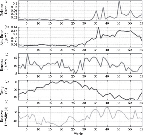
FIGURE 2.1 Benzene concentration estimation results in the 10-day training length run (weekly averages): (a) MRE; (b) MAE; (c) benzene concentrations as measured by a conventional station; (d) temperature measured by multisensor device; (e) relative humidity measured by the multisensor device. Results are affected by what we expect to be seasonal meteorological effects, evident after the 30th week (starting in November) superimposed to a slow degradation due to sensor aging effects (drifts). After the 50th week, the absolute error shows a definite recovery trend.
Sensor recalibration is needed and has been found to be very efficient but, since the number of multisensory devices to deploy is very high, conventional recalibration procedures employing reference gases or on-field approaches cannot be easily implemented. State-of-the-art drift correction algorithms, acting to subtract drift contribution to sensor responses, can obtain very interesting results but need a significant number of samples themselves in order to ground the value of their free parameters. Recently, we have started to investigate the use of semisupervised learning techniques as a way to solve this problem adaptively that could be classified as a dynamic pattern recognition problem (see Figure 2.2) [10]. In fact, distributed architectures often are built with sensing nodes that sport relevant but unused computing capabilities; this can provide diagnostic services and allow the possibility to self-improve the stability of sensor metrological characteristics. In particular, this can be significant for implementing drift adaptation strategies, accommodating this paramount problem in solid-state chemical sensing.
In networked configurations, sensor recalibration could also be performed cooperatively by temporarily adding other moving reference sensors or, thanks to data fusion techniques, using mutual recalibration strategies. Practically, the development of application-specific algorithms could allow mutual calibration by exploiting networked cooperation in a totally unmanned fashion. In a work from Tsujita and co-workers [11], a network of NO2 sensors recalibrate their baseline response by exploiting the identification of baseline conditions (very low NO2 concentrations) by cooperating sensors’ responses and particular conditions (dawn at low humidity and reference temperature).
FIGURE 2.2 Drift counteraction with semisupervised learning. CO estimation comparison with SSL (secure sockets layer) algorithm (dark line) and standard neural network algorithm (light line) based on only 24 training samples (1 day). The SSL approach achieved an 11.5% performance gain with respect to the 1-year long averaged MAE score.
Anyway, sensor drift still remains a significant issue that prevents the spread of the use of multisensing devices in urban pollution scenarios. Future directions of research include a combination of advanced signal processing techniques and sensing capability improvement reducing both nonspecificities and sensor drift. Calibration transfer strategies are also to be developed to cope with sensor production issues like inhomogeneity.
The process of the development of battery-operated WCSNs cannot avoid addressing the power consumption issue. State-of-the-art metal oxide (MOX) chemical sensors require high working temperatures for best sensitivity and specificity [12]. This issue limits the possibility of using them in wireless chemical sensing motes because their average power consumption is in the range of hundreds of milliwatts with continuous operation allowing only for a limited life span in battery-operated nodes. Instead, polymer-based chemiresistors, resonators, and mass sensors (QMBs, SAWs) are usually operated at room temperature [13]. Although they are not as common as their MOX counterparts, their low power operation capability can be recognized as a huge advantage with respect to the other technologies, especially when VOC (volatile organic compound) detection is concerned [14,15]. Unfortunately, they may not be as efficient at very low concentrations and most of them are significantly affected by humidity and heavy drift [16].
For a decade, polymer/nanocomposite reactivity to chemicals has also been applied to the development of passive resonant sensors that are capable of wireless remote operations in a very simple way. LED/polymer-based optical sensing can be an extremely interesting solution for all applications where high limits of detection are not an issue because of very low cost, reliability, and very low power demand [17]. However, in order to obtain suitable sensitivity in most applications, laser sources should be used, and this may increase both costs and power needs significantly.
From the architectural point of view, current commercial e-noses are not designed to tackle distributed chemical sensing problem especially with regards to power management, however during last years a number of novel approaches have been proposed and experimented. This field is hence rapidly evolving exploiting the plethora of results obtained by researchers in wireless technology field. As an example, Bicelli et al. [18] have investigated the use of commercial low power MOX sensors in a WSN network for indoor gas detection applications. They first suggested employing a specially designed pulsed heating procedure in an attempt to achieve a significant increase in the wireless sensor battery life (about 1 year) with a sample period in the range of 2 minutes. Their results showed a serious trade-off between total power consumption and actual response time [18]. Pan et al. realized a single w-nose for online monitoring of livestock farm odors integrating meteorological information and wind vector [19]; detection performances and power consumption have not been reported, so it was not possible to estimate autonomous life expectation. Becher et al. recently presented a four MOX sensor-based WCSN network for flammable detection in military docks, but again, power needs restricted the application to the availability of power mains [20].
During the last years, our WCSN commitment focused on the development of a wireless electronic nose platform called TinyNose [21], based on commercially available WSN motes and controlled by software components relying on the TinyOS operating system [22]. The platform makes use of four room-temperature operating low power polymeric chemical sensors that extend the entire sensory network life span at the cost of a low sensitivity. When low power sensors are used, radio power becomes significant in the overall power budget of the platform. In a 2011 work, we focused on the possibility of using computational intelligence algorithms in order to further extend the network life span by implementing a sensor censoring strategy (see references 23–24,25) focused on allowing the transmission of informative data packets neglecting uninformative data [26]. The target scenario for the application of the proposed methodology was the distributed monitoring of indoor air quality and, specifically, the detection of toxic/dangerous VOC spills. The same architecture has been used to develop and test an ad hoc algorithm for real-time 3D gas mapping with a WCSN in indoor simulated environments so as to extract the needed semantic content from the deployed network [27].
Specifically, our platform relies on the use of nonconductive polymer/carbon black sensors whose sensing mechanism of response is, at its simplest level, based on swelling. When the isolating polymer film within which conductive particles have been dispersed is exposed to a particular vapor, it swells while absorbing a varying amount of organic vapors depending on polymer type. The swelling disrupts conductive filler pathways in the film by pushing particles apart and the electric resistance of the composite increases [15].
In order to obtain a suitable voltage signal (i.e., showing proportionality to sensor resistance variation), a simple amplified resistance to voltage converter signal conditioning system was implemented. Suitable choice of circuit parameters allows the proper operation of the board within a wide range of base resistance. In Figure 2.2, a simplified functional scheme of the board is shown.
The overall sensing subsystem was then directly connected to four A/D input ports provided by the core mote of the proposed platform, the commercial Crossbow TelosB mote—a research-oriented mote platform that has shown its operative potential over time [28]. Powered by 2 AA batteries, the chosen platform is based on a low power T I MSP430F1611 RISC microcontroller w featuring 10 kB of RAM, 48 kB of flash, and 128 B of information storage. The embedded low power radio, Chipcom CC2420, represents the kernel for 802.15.4 protocols’ stack support.
The heterogeneity of the practical applications and the limited energy availability required a careful design of the software (sw) structure and protocols for the management of the wireless e-nose platform. The TinyOS operating system guaranteed the possibility to keep the focus on domain-specific optimization and, in particular, the implementation of the sensor censoring strategy.
TinyOS is an open-source operating system for WSN applications developed by the University of California at Berkeley [22]. Essentially, its component library includes network protocols, distributed services, basic sensor drivers, and data acquisition tools—all of which can be further refined for custom applications. Specific software modules allow for the basic management of the sensor node, like local I/O and radio transmissions. Furthermore, the power management model of TinyOS allows for the automatic management of module subsystems switching among active, idle, and sleep phases, achieving a generalized power management strategy
A C-derived language, NesC, is the reference programming language for TinyOS-based programming. NesC relies on a component-based programming module.
Figure 2.3 shows a UML deployment diagram of the overall platform software architecture from which its three-layer design is clearly apparent. The first layer encompasses all the embedded sw components developed in NesC and providing local control of the pneumatic section of the electronic nose (if available), sensor interface control, data acquisition and processing, and, eventually, data transmission capabilities. At the second layer, a PC-based component coded in Java captures data packets from a sensorless node that act as a gateway toward the IP-based network and storage facilities. At the third level, multiple graphical user interfaces (GUIs), also coded in Java, can provide visualization and recording features while remotely controlling relevant parameters for embedded sw operations (e.g., duty cycle parameters).
Actually, the overall architecture has been designed to host two pattern recognition and sensor fusion layers. The first layer defines methods to connect a sensor’s raw data processing component that will allow for local situation awareness. It was connected to the local sensor fusion component that allows for the local estimation of pollutant concentrations by using a trained neural network (NN) algorithm. The second layer provides second-level sensor fusion services, allowing for integrating estimation coming from all the deployed nose. This level is responsible for the cooperative reconstruction of an olfactive image of the environment in which they are deployed.
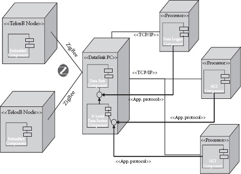
FIGURE 2.3 UML deployment diagram of the software architecture for the proposed platform.
2.4 DUTY CYCLE AND POWER CONSUMPTION
The TinyNose node has been designed for continuous real-time monitoring of volatiles with a programmable duty cycle, including sensor data acquisition, processing, and transmission toward a data sink. Duty cycle parameters and, in particular, the length of each phase and the sampling frequency are fully programmable by the application designer; sample frequency can be set dynamically at run time by GUI. In order to characterize the power consumption fully, we can easily separate the duty cycle into four separate phases, each one having different power needs:
• Sleep phase. In this phase, each node is put to sleep. MCU and radio are turned into stand-by mode.
• Sensing phase. Sensors driving, data acquisition, and ADC conversion are carried out.
• Computing phase. Data processing is performed in order to prepare data to be transmitted toward a data sink.
• Transmission/reception phase. The actual data transfer takes place.
Battery life can be optimized by controlling the duration of each phase and the activation of sensors driving electronics.
At any instant, a single module power consumption can be computed as a function of its microcontroller power state; whether the radio, pump, and sensor driving electronics are on; and what operations the active MCU subunits are performing (analog to digital conversion). By using appropriate programming models (e.g., relying on split-phase operations), it is possible to best utilize the features provided by TinyOS to keep the power consumption to a minimum. In particular, with regard to radio stack management, we have chosen to rely on the LPL (low power listening) algorithm [22]. As such, node radio can be programmed to switch on periodically just long enough to detect a carrier on the channel. If a carrier has been detected, then the radio remains on long enough to detect a packet to be routed to the data sink for mesh shaped networking. After a timeout, the radio can be switched off.
In order to assess the base consumption of the TinyNose platform, a measuring setup based on a Tektronix TDS 3032 digital oscilloscope was set to measure Vshunt on 10 Ω shunt resistance and to let us derive current. Actually, in its simplest configuration with sample frequency set at 1 Hz, the sensor node, as mentioned before, remains in sleeping mode for most of the time (TRS time interval). In this phase, a current, IRS, measured as 12 μA, is drawn. During the TWR wake-up period, the sensor node turns on the chip radio awakening from the sleep mode. In this stage, we measured a 5 mA mean current draw. After that, the system sets up itself for data capture and conversion with a mean current draw of 19 mA. Even in this stage, provided that data are sent every acquisition cycle, radio activity is the main source of power consumption. In fact, power consumption, in the active phase, is dominated by radio activity until switch-off timeout inset; after ADC converter timeout, it can be measured as 18 mA. Eventually, the radio frequency circuit is turned off again and the state changes from transmission mode to sleeping mode.
Figure 2.4 shows the detailed evolution of the TelosB drawn current during acquisition, processing and data transmission of sensor data, while Table 2.1 shows the consumption in terms of measured currents during each operating phase. Because of the high consumption of the prototype signal condition board (38 mA), a digital signal drives a switch that lets the electronics board power supply to be switched on only during the data capture time slice. This strategy is made possible by a polymer sensor sensing mechanism; in fact, polymer swelling is only negligibly affected by actual sensor power up so that sensors do not need warming up before their resistance can be sampled (see Table 2.2).
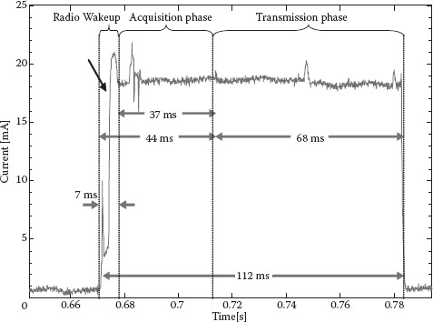
FIGURE 2.4 Current absorbed by TelosB in its active operating phase—in particular during the radio wake-up, sensing, and transmission phases in a complete cycle.
TABLE 2.1
Core Mote Consumption in Different Phases of the Duty Cycle
Operation phase |
Time (m) |
Current request (mA) |
Radio sleep (RS) |
TRS = 888 |
IRS = 0.012 |
Radio wake-up (RW) |
TRW = 7 |
IRW = 5 |
Acquisition (A) |
TA = 37 |
IA = 19 |
Computing (C) |
TC = 25 |
IC = 2.5 |
Transmission (T) |
TT = 68 |
IT = 18 |
TABLE 2.2
Platform Signal Conditioning Board Consumption
Operation phase |
Time (ms) |
Current request (mA) |
Operating condition |
TON = 30 |
38 |
Usually, module life span can be estimated using the mean current consumption—namely, Icc,mean—of the wireless sensor, considering battery capacity, conversion efficiency, and power supply output voltage gain.
The mean current value (Icc,mean) obtained under the basic operating conditions without applying sensor censoring can be computed according to Equation (2.1) by using the current measured in the proposed setup:
(2.1) |
Neglecting conversion efficiency, battery life (BL) can be computed as a function of the battery capacity, C, and total current draw. For our w-nose, C is equal to 3500 mAh, while total current is equal to the sum of mean current absorbed by conditioning board Ib, mean (30/1000 * 38 = 1.14 mA) and the Icc, mean (1.97 mA computed using Equation 2.1). Expressing BL as the ratio C/(Icc,mean + Ib,mean), we can estimate that the overall e-nose battery life, with sampling and transmission frequency of 1 Hz, is roughly 47 days—a rather interesting value for a four-sensor four-nose. Extending the sample period to 10 s, hence losing real-time characteristics, this basic setting will account for a battery life in excess of 1 year.
2.5 POWER SAVING USING SENSOR CENSORING
The additional power required for the execution of the local data processing components should be seriously taken into account in order to evaluate the benefits of censoring strategies. However, the outcome depends basically on the rate of significant events’ occurrence; in most chemical sensing scenarios, the probability, p, of a significant event to occur (e.g., chemical spills) is expected to be very low, while the timely transmission of relevant data is needed in security applications.
In order to perform an experimental check of the sensor censoring concepts in WCSN scenarios, we designed and implemented an ad hoc lab-scale experiment. A sensor fusion component that was trained for a distributed pollutant detection application was developed and the power savings obtained by using sensor censoring were evaluated. Actually, we assumed a general chemical sensing problem characterized by the presence of two pollutants whose toxic/dangerous concentration limits were different. To save battery energy, the single mote should be able to decide whether to transmit or not the sampled data on the basis of the concentration of the two gases estimated by sensor responses. The e-nose sensor arrays were exposed to different concentration levels of acetic acid in a controlled environment setup, and their responses, sampled by the motes, were recorded to build a suitable data set for the training of an ANN component to be run onboard. ANN architecture was chosen on the basis of considerations about its flexibility, high capacity, compact knowledge representation (low space footprint), and low computational demands. The onboard component was then loaded with network weights obtained by training an identical model in MATLAB with the recorded data set so as to reach a reasonable point-to-point real-time estimation of concentrations of different analytes.
The proposed architecture performance was evaluated by dividing validation set mean absolute error (MAE) by analyte concentration range span, obtaining a 6% (standard deviation: 10%) value for the acetic acid concentration estimation problem and 11% (standard deviation:11%) for the ethanol problem (see Figure 2.5).
Following a measurement approach, the execution of the NN sensor fusion component accounts for additional 2.5 mA consumption over a total time span of 25 ms (function call overhead included). See Tables 2.3 and 2.4.
In order to reassess total power consumption, we write Equation (2.1) again by taking into account the computing phase:
(2.2) |
FIGURE 2.5(A) Acetic acid concentration estimation (bottom) performed by the FFNN (feed forward neural network) component plotted against true concentration (top). The x-axis depicts time (samples) while the y-axis depicts real and estimated concentration values.
FIGURE 2.5(B) Ethanol concentration estimation (bottom) performed by the FFNN component plotted against true concentration (top). The x-axis depicts time (samples) while the y-axis depicts real and estimated concentration values.
This equation provides the mean current supplied by the batteries in case of significant event occurrence: The mote performs signal conditioning and data sampling, data fusion by means of NN, and data transmission every T seconds.
Using a Bernoulli random variable X ~ B (1, p), which would model the result of the computation performed by the NN to verify whether the acquired data have been transmitted on the radio channel, Equation (2.2) can be rewritten as
(2.3) |
where and are respectively:
(2.4) |
By exploiting Equation (2.3), we can finally discuss the advantages of NN-based sensor censoring for the implementation of power saving strategies in the proposed architecture.
TABLE 2.3
Memory Footprint Increase in Embedded Component Resulting from Linking of Sensor Fusion Neural Component
Algorithm |
Bytes in ROM |
Bytes in RAM |
Basic |
20,380 |
574 |
Basic + NN comp. |
27,340 |
910 |
TABLE 2.4
Computational Complexity in terms of functional calls
Functional |
Calls per each NN estimation |
Tanh |
10 |
Multiplication |
76 |
Sum |
82 |
The worst case is obtained when p = 1; that is, when all samples refers to significant events, then the mean current computed using Equation (2.3) is obviously greater than the one calculated by Equation (2.1) (i.e., )However, by equating Equations (2.1) and (2.3) and selecting p as independent variable, we obtain:
(2.5) |
The obtained value represents the percentage threshold of a significant event under which the NN-based sensor censoring becomes more efficient with regard to power management. This computed threshold level makes the use of the proposed approach feasible for most of the analyzed distributed chemical sensing scenarios.
In monitoring industrial chemical spills, even considering false-positive generation, it is reasonable to expect values of p that reflect only a few significant samples a day. Of course, censoring criteria (i.e., the “spiking” threshold) should be chosen exploring the trade-off among sensitivity and the false-positive rate caused by estimation errors, also considering the danger/toxicity level of the target gas. For an experimental evaluation, using the previously mentioned setup and allowing a small slack to the network estimation of ethanol (detection threshold on NN response = 10 ppm with respect to a 2000 ppm max exposure level), we obtain a false positive rate of 5% for ethanol and less than 1% for acetic acid. In a case of no positive events during node lifetime—a reasonable expectation in safety oriented leakage detection scenario—a proposed node can be expected to experiment a maximum operative life span that is very near to the intrinsic limit now dominated by the power needed by a signal conditioning board. In particular, considering p = 0.01, the expected lifetime computed by taking into account Equation (2.3) reaches 113 days (110 days for p = 0.05)—a rather interesting value for a four-sensor wireless electronic nose with real-time operating characteristics.
As stated in the introduction, the capability to reconstruct 3D gas mappings is becoming more and more interesting for the possible applications in city air pollution mapping, hazardous gas spills’ localization, and energy efficiency (e.g., efficient control of heating, ventilation, and air conditioning [HVAC] automation in buildings). Recently, we investigated the possibility of obtaining 3D quantitative indoor air quality assessment with the TinyNose architecture [27]. The outcome revealed the capability of building gas concentration mapping of acetic acid–ethanol mixtures (as VOC pollutant simulants) in ambient air with the mesh of four w-noses coupled with a two-stage sensor fusion system. In order to focus on the 3D reconstruction problem, a set of four TinyNose w-noses equipped with a four MOX sensor array has been considered. A basic performance estimation procedure has been conducted on a single TinyNose equipped with the novel MOX-based sensor array. The node was exposed using a controlled climatic chamber to different concentrations of acetic acid and ethanol at different relative humidity percentages (see Table 2.5). By using sensor responses, a two-slot tapped delay neural network (TDNN) with 10 hidden layer neurons for instantaneous concentration estimation obtained a MAE/range value of 2.34% (0.75 ppm) for acetic acid and 6.5% (9.8 ppm) for ethanol (see Figure 2.6).
However, following an on-field approach to calibration, we decided to design a second experimental setup involving the deployment of a network of four instances of TinyNose in an ad hoc glass box (volume = 0.36 m3) and evaluate their capability to reconstruct a real-time 3D chemical concentration image of the two previous pollutants. Different amounts of the two chemicals (see Table 2.6) were introduced and diluted until complete evaporation with the use of a standard PC fan. Based on the reasonable hypothesis of uniform concentration distribution over the box, at steady state, the response of the node was sampled (1 Hz) to build a suitable data set for the training of the TinyNoses. This was based on a two-level classifier/regressor scheme. In this way, each of the w-noses was made capable of estimating the local pollutant concentration at its deployment location. Further, 10 runs of steady-state sample acquisition with the same procedure were then used to build a suitable test set. The test set MAE, averaged for all four w-noses, reached 3.15 and 4.36 ppm for ethanol and acetic acid, respectively. These figures allow us to locate the expected absolute error on the real-time local concentration estimation under a 5 ppm threshold. This value is valid for concentration estimation in a mixture and thus in the presence of interferents, provided that concentration levels have a slow variation rate.
TABLE 2.5
Controlled Chamber Experimental Setup
Gas concentration ranges |
||
RH (%) |
Acetic acid (ppm) |
Ethanol (ppm) |
[20, 30, 50] |
[0, 5, 7, 10, 15, 20, 25, 30, 32] |
[0, 15, 30, 70, 90, 115, 130, 150] |
Notes: The different gas mixtures used during the experimental setup were synthesized by using all combinations of the reported concentrations of acetic acid and ethanol at different relative humidity concentrations for a total of 216 cycles. The baseline mixture was set at RH = 50%.
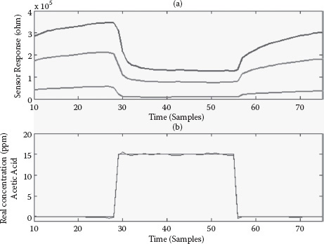
FIGURE 2.6 (a) Sensor array responses in controlled chamber setup; (b) trained TDNN responses and ground truth comparison during the correspondent complete exposure cycle.
TABLE 2.6
Glass Box Experimental Setup
Gas concentration ranges |
|
Acetic acid (ppm) |
Ethanol (ppm) |
[0, 5, 10, 15, 20] |
[0, 6, 12, 17, 23] |
Notes: The different gas mixtures used during the glass box experimental setup were synthesized by using all combinations of the reported concentrations of acetic acid and ethanol. For each combination, two different exposure cycles were executed. The steady-state sensor array response to each exposure cycle was recorded to build the training data set. Ambient RH values and temperatures (not controlled) were also recorded to be part of the on-board feature set.
In order to reconstruct a 3D chemical image of the glass box, the kernel-DV algorithm (see Nakamoto and Ishida [3]), originally developed by the Lilienthal group for use with mobile robot acquisitions, was adapted for real-time cooperative sensor fusion. The algorithm basically used a 3D Gaussian kernel to propagate localized measurement to a 3D environment based on confidence values depending on the point distance from the actual measurement points. Estimation based on the kernel propagation was balanced with a default averaged value (homogeneous gas distribution) by the use of the confidence value that is normalized by a scale factor. Eventually, should confidence value fall to 0 (points located far from all actual measurement points), the algorithm reverts to the homogeneous gas distribution hypothesis. In the last setup, 17 μg of ethanol was allowed to evaporate within the glass box in one of the left-down box corner. By using the neural calibration obtained before and encoded in the on board computational intelligence component, the single nodes were able to estimate local concentration of both gases. Their estimations were transmitted and collected at a data sink, where a sensor fusion component was coded to reconstruct an instantaneous 3D chemical image of the box.
Overall performance of the 3D reconstruction algorithm depends on the value of three base parameters of the kernel-DV algorithm (i.e., cell mesh width, the kernel width σ, the confidence scale parameter, and, of course, by the w-nose deployment positions. Cell mesh width only trades off 3D reconstruction resolution with computational costs; for this reason, a fixed value that allows for real-time reconstruction has been selected. The confidence scale parameter depends on kernel width, so, for a fixed deployment configuration of the w-noses, an automated procedure has been designed to choose the appropriate kernel width parameter value on the basis of a leave-one-mote-out approach. Actually, in scanning a parameter value array ([0.05, 0.10, 0.15, 0.2]) for each parameter setting, all but one sensing node have been used to estimate the concentration value of the two analytes, with the adapted kernel-DV algorithm at the remaining node position. Figure 2.7(a) shows the comparison between local instantaneous concentration estimation at node position 3 and estimation carried out by the 3D reconstruction algorithm at the same position. Without affecting generalization, the mean absolute difference between the estimated value and the actual value as estimated by the remaining node, during all the exposure time, has been defined as the performance value to be optimized by the brute force approach.

FIGURE 2.7(A) Instantaneous ethanol concentration estimation as computed at node 3 (top) compared with the estimation obtained by 3D reconstruction, using the remaining three nodes, at the same location. The experimental setup foresees the deployment of four w-noses in the 0.36 m3 glass box and the release of 17 mg (20.9 ppm) of ethanol near one corner of the box.
FIGURE 2.7(B) Instantaneous absolute difference among local ethanol concentration and 3D reconstruction algorithm with kernel width s set at 0.1 value. The instantaneous difference reported here was averaged throughout the leave-one-mote-out procedure executed for the exposure to 17 mg (20.9 ppm) of ethanol. The computed MAE value was used for the optimization of the 3D reconstruction algorithm.
Figure 2.7(b) shows the averaged instantaneous absolute difference among local and 3D reconstruction-based estimations for the four motes in the ethanol case. Peaks can be spotted in the rise and fall of the concentration levels during transients. The peaks can be explained by the different concentrations experimented with by the motes during transients due to their different positions. In this case, the peaks’ magnitude could be effectively reduced by tuning mote positioning and density of the measurement mesh in the sensed environment. Figures 2.8 and 2.9 depict, respectively, w-nose positioning and an instantaneous reconstruction of the concentration of the two pollutants. This preliminary result shows the possibility of effectively using a w-nose deployment for real-time 3D quantitative air quality analysis in the presence of a pollutant mixture. The use of mote cross validation has also been shown for the sensor fusion algorithm parameter tuning and performance evaluation.
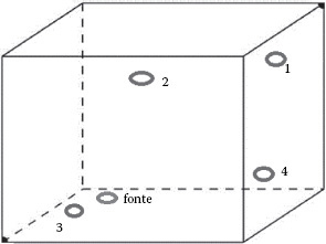
FIGURE 2.8 Positioning of the four w-noses and gas source within the glass box.
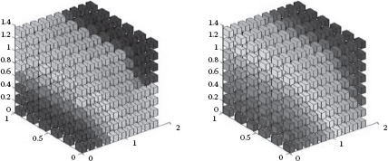
FIGURE 2.9 Instantaneous 3D ethanol (right) and acetic acid (left) concentration reconstruction (computed at data sink) using a four w-nose deployment in the glass box experimental setup.
WCSN architectures can provide a new insight on important and potentially life-saving phenomena like the detection of pollutants and/or hazardous gas. Their practical diffusion is still limited by several issues, like power management and sensors’ nonspecificity and instability. Ad hoc 3D diffusion models can be devised to obtain high level semantic information about gas concentrations with applications to spill localization or energy efficiency (HVAC automation).
In both cases computational intelligence, together with distributed sensing techniques, may allow for viable solutions—even in the case of using low cost equipment exploiting redundancy and the power of machine learning. Since 2006, our research group, together with several researchers all around the globe, has been committed to the development of solutions for real-world applications that could be engineered to the market. Despite the growing number of contributions in this field, the main issues are still there and appear to be solved only for specific segments of a complete application. Our efforts have produced a complete platform, called TinyNose, that allows us to address all the applicative segments of WCSN architecture. Currently the development of WCSNs is rapidly progressing toward real-world applications; however, the massive on-field testbed deployments needed to test their reliability in indoor and outdoor scenarios are still to be realized.
Core work for this chapter has been conducted by researchers at UTTP-MDB lab of the ENEA Centro Ricerche Portici. For cooperation and support, I am indebted to my co-workers and in particular to E. Massera, G. Fattoruso, G. Di Francia, and M. Miglietta.
1. D. Dockery, C. A. Pope, X. Xu, F. Speizer, J. Schwartz. An association between air pollution and mortality in six US cities. New England Journal of Medicine 329:1753–1759 (1993).
2. C. Grimes, K. G. On, O. K. Varghese, X. Yang, G. Mor, M. Paulose, E. C. Dickey, C. Ruan. A sentinel sensor network for hydrogen sensing. Sensors 3:69–82 (2003).
3. T. Nakamoto, H. Ishida. Chemical sensing in spatial/temporal domains. Chemical Review 108 (2):680–704 (2008).
4. J. Achim, A. L. Lilienthal, T. Duckett. Airborne chemical sensing with mobile robots. Sensors 6:1616–1678 (2006).
5. J. Achim, A. L. Lilienthal, T. Duckett. Building gas concentration grid maps with a mobile robot. Robotics and Autonomous Systems 48 (1):3–16 (2004).
6. S. De Vito et al. TinyNose: Developing a wireless e-nose platform for distributed air quality monitoring applications. IEEE Conference on Sensors, Oct. 26–29, Lecce, Italy, pp. 701–704 (2008).
7. R. Shepherd, S. Beirne, K. T. Lau, B. Corcoran, D. Diamond. Monitoring chemical plumes in an environmental sensing chamber with a wireless chemical sensor network. Sensors and Actuators B: Chemical 121 (1):142–149 (2007).
8. I. F. Akyildiz, W. Su, Y. Sankarasubramaniam, E. Cayirci. Wireless sensor networks: A survey. Computer Networks 38:393–422 (2002).
9. S. De Vito, E. Massera, M. Piga, L. Martinotto, G. Di Francia. On-field calibration of an electronic nose for benzene estimation in an urban pollution monitoring scenario. Sensors and Actuators B: Chemical 129 (2):750–757 (2007).
10. S. De Vito, G. Fattoruso, M. Pardo, F. Tortorella, G. Di Francia. Semi-supervised learning techniques in artificial olfaction: A novel approach to classification problems and drift counteraction. IEEE Sensors Journal 12:3215–3224 (2012).
11. W. Tsujita, A. Yoshino, H. Ishida, T. Moriizumi. Gas sensor network for air-pollution monitoring. Sensors and Actuators B: Chemical 110:304–311 (2005).
12. N. Barsan, U. Weimar. Conduction model of metal oxide gas sensors. Journal of Electroceramics 7 (3):143–167 (2001).
13. K. Arshak, E. Moore, G. M. Lyons, J. Harris, S. Clifford. A review of gas sensors employed in electronic nose applications. Sensor Review 24 (2):181–198 (2004).
14. L. Quercia, F. Loffredo, B. Alfano, V. La Ferrara, G. Di Francia. Fabrication and characterization of carbon nanoparticles for polymer based vapor sensors. Sensors and Actuators B 100:22–27 (2004).
15. E. J. Severin, B. J. Doleman, N. S. Lewis. An investigation of the concentration dependence and response to analyte mixtures of carbon black/insulating organic polymer composite vapor detectors. Analytical Chemistry 72:658–668 (2000).
16. S. C. Ha, Y. Yang, Y. S. Kim, S. H. Kim, Y. J. Kim, S. M. Cho. Environmental temperature independent gas sensor array based on polymer composite. Sensors and Actuators B 108:258–264 (2005).
17. D. Diamond, S. Coyle, S. Scampagnani, J. Hayes. Wireless sensor networks and chemo-/biosensing. Chemical Reviews 108 (2):652–679 (2008).
18. S. Bicelli et al. Model and experimental characterization of the dynamic behavior of low-power carbon monoxide MOX sensors operated with pulsed temperature profiles. IEEE Transactions Instrumentation and Measures 58 (5):1324–1332 (2009).
19. L. Pan et al. A wireless electronic nose network for odors around livestock farms. Proceedings of 14th M2VIP 2007, Xiamen, pp. 211–216 (2007).
20. C. Becher, P. Kaul, J. Mitrovics, J. Warmer. The detection of evaporating hazardous material released from moving sources using a gas sensor network. Sensors and Actuators B: Chemical 146 (2):513–520 (2010).
21. S. De Vito et al. Power savvy wireless e-nose network using in-network intelligence. Proceedings of 13th ISOEN, AIP Conference Proceedings 1137:211–214. ISBN: 978-0-7354-0674-2.
23. C. Rago, P. Willett, Y. Bar-Shalom. Censoring sensors: A low-communication rate scheme for distributed detection. IEEE Transactions Aerospace Electronics Systems 32 (2):554–568 (1996).
24. S. Appadwedula, V. V. Veeravalli, D. L. Jones. Decentralized detection with censoring sensors. IEEE Transactions on Signal Processing 56 (4):1362–1373 (2008).
25. E. Y. Chang, A. Jain. Adaptive sampling for sensor networks. Proceedings of First International Workshop on Data Management for Sensor Networks, DMSN, August 30, Toronto, Canada, 72:10–16 (2004).
26. S. De Vito, P. Di Palma, C. Ambrosino, E. Massera, G. Burrasca, M. L. Miglietta, G. Di Francia. Wireless sensor networks for distributed chemical sensing: Addressing power consumption limits with on-board intelligence. IEEE Sensors Journal 11 (4):947–955 (2011).
27. S. De Vito et al. Cooperative 3D air quality assessment with wireless chemical sensing networks. Procedia Engineering 25:84–87
28. J. Polastre, R. Szewczyk. Telos: Enabling ultra-low power wireless research. Proceedings International Symposium on Information Processing in Sensor Networks, pp. 364–369 (2005).