Chapter 8 Efficient MIMO Receiver Design for Next Generation Wireless Systems

Recently, there has been growing interest in spatial multiplexing (SM) for multiple-input multiple-output (MIMO) systems since it can increase the data rate linearly with the number of antennas [1]. To achieve the promised gain of MIMO SM, it is crucial to handle the interference among multiple spatial streams wisely. Given the channel knowledge at the transmitter, the spatial streams can be precoded such that interference among multiple streams at the receiver is mitigated. The required channel knowledge is fed back from the receiver to the transmitter. However, it is not easy to obtain the perfect channel knowledge at the transmitter. For example, when the channel fluctuates rapidly, the amount of feedback from the receiver becomes prohibitively high. Since it is difficult to achieve the instantaneous channel knowledge perfectly at the transmitter, correspondingly there is a limit to cancelling the interference at the transmitter. Instead, it is necessary for a receiver to handle the interference among spatial streams with ease of obtaining the channel knowledge. Thus, the design of an intelligent receiver becomes critical.

This chapter introduces the advanced SM detection scheme over conventional detection schemes. Section 8.1 describes the trend on MIMO systems in recent standards. Section 8.2 explains basic principles of SM technologies for both single-user and multiuser SM, the advanced detection combined with decoding on SM, and the introduction of both hard- and soft-detection receivers. In Section 8.3, various SM detection schemes are depicted, such as equalization-based schemes and maximum likelihood (ML) schemes. In particular, we develop an ML detection algorithm named dimension reduction soft detector (DRSD) that achieves the near-ML performance with a significantly lower complexity than existing receivers. Finally, an iterative detection and decoding (IDD) scheme, which recently has attracted more attention due to higher performance at the cost of additional complexity, is discussed.

8.1 RECENT TRENDS ON MIMO SYSTEMS

MIMO technologies have been adopted rapidly in wireless communications since they can significantly increase data throughput or reliability without paying the cost of additional bandwidth or additional power at the transmitter. Such a potential benefit is achieved by distributing the same total transmit power over multiple antennas. These MIMO technologies lead to an array gain or diversity gain that improves the spectral efficiency or link reliability, respectively. SM techniques increase data rate performance by simultaneously sending multiple streams of information. If these signals arrive at the receiver with sufficiently different spatial signatures, the receiver can separate these streams into parallel channels. On the other hand, spatial diversity (SD) techniques enable the streams to be reliable and the coverage to be enhanced on the received signal by sending redundant streams of information. The received signal coming from multiple paths causes it to be less likely that all of the paths are simultaneously degraded [2]. As a result, MIMO techniques along with SM and SD increase the minimum cell spectral efficiency, the cell edge user spectral efficiency, and the peak spectral efficiency, all of which are considered as important quality of service parameters [3]. Because of these benefits, multiple antenna techniques are widely used in various modern wireless communication standards such as IEEE 802.11n, third generation partnership project (3GPP), long term evolution (LTE), worldwide interoperability for microwave access (WiMAX), high speed packet access plus (HSPA+), and so forth.

8.1.1 CELLULAR SYSTEMS

The IEEE 802.16e (i.e., WiMAX Profile 1.0) and 3GPP evolved universal terrestrial radio access (E-UTRA) LTE (releases 8 and 9) standards have been developed so as to be a part of the IMT-2000 third generation (3G) technologies [4]. IEEE 802.16m (WiMAX Profile 2.0) and 3GPP E-UTRA LTE-advanced (LTE-A) (release 10 or beyond) are two evolving standards targeting 4G wireless systems to meet or exceed the requirements of ITU 4G technologies [5,6], where MIMO technologies play an essential role in meeting 4G requirements. They not only enhance the performance of the conventional point-to-point link, but also effectively support multiuser channels such as broadcast channels and multiple access channels through multiuser MIMO. A large family of MIMO techniques has been developed for various links and modes, including space frequency block coding (SFBC), frequency-switched transmit diversity (FSTD), cyclic delay diversity (CDD), and open-loop and closed-loop beam-forming and precoding [7]. For example, 802.16m and LTE-A MIMO schemes have various configurations of two, four, or eight transmit antennas and a minimum of two receive antennas in the downlink, and one, two, or four transmit antennas with the minimum of two receive antennas in the uplink, where up to eight streams can be transmitted for a single-user downlink SM [2,11].

8.1.2 WIRELESS LAN AND PAN

One of the most prominent features in IEEE 802.11n, which was ratified in 2009, is the MIMO capability. A flexible MIMO concept allows the array of up to four antennas. These multiple antennas enable use of SM or beam-forming technologies along with wider bandwidths and a number of MAC layer algorithms that achieve a peak theoretical throughput in the order of 600 Mbps [8]. Since the ratification of 802.11n, a new task group, 802.11ac, has worked on the next standard for even higher throughput within 6 GHz spectra. New features in this standard include the bandwidths of 80 and 160 MHz, while 802.11n offered only 40 MHz; 256 quadrature amplitude modulation (QAM); up to eight antennas; and multiuser MIMO.

Another task group, 802.11ad, is looking at very high throughput (e.g., 7 Gbps) for spectrum at 6 GHz or higher frequency such as the 60 GHz ISM band. Besides 802.11ad, several standards have been introduced in the 60 GHz band, such as IEEE 802.15.3c, WirelessHD, Wireless Gigabit Alliance (WiGig), and ECMA-387 [9]. With much shorter wavelength at 60 GHz, MIMO techniques are extended to overcome the range issue through beam-forming algorithms with tens of or more antennas. For instance, a 32 × 32 antenna array can be implemented on a CMOS (complementary metal oxide semiconductor) process. Similarly, a large number of receive and transmit chains required for such a system are pushing the standards committee to consider MIMO techniques other than beam-forming techniques such as space-time block coding (STBC) [10].

8.2 BASIC MIMO SM TECHNOLOGIES

This section mainly discusses transmitter and receiver technologies for SM MIMO. The SM transmission can be classified into single-user and multiuser SM where spatial streams are allocated to a single user or multiple users, respectively. At the receiver, the detection of the received signal is first applied and optionally followed by decoding the detected output bits when channel coding is employed. Whether the detection delivers a hard symbol, one of the candidate symbols determined on the constellation, or a soft symbol, the likelihood for each message bit calculated instead of being determined to the decoder, the detection is categorized into hard and soft detection, respectively. These basic concepts regarding the SM detection and decoding are to be explained in detail in the following.

8.2.1 SINGLE-USER AND MULTIUSER SM

In single-user SM, all the spatial streams are allocated to a single-user. They are used in conjunction with beam-forming techniques to maximize the throughput. As higher peak throughput is required, the larger number of streams has been exploited to meet the requirement. The advanced receiver technology enables achieving such a requirement in practice. For example, it is known that the higher order modulation substantially increases the peak data rate. The recently implemented receiver starts to support such a higher order modulation with a reliable error rate. On the other hand, SM techniques in a multiuser scenario deliver data streams in a spatially multiplexed fashion to different users. Under these techniques, all the degrees of freedom of a MIMO system are known to be achieved. These SM techniques operate with the idea that the applied multiuser beam-forming or precoding schemes cause the radiation pattern of the base station to be adapted to each user for obtaining the highest possible gain in the direction of the user. Akyildiz, Gutierrez-Estevez, and Reyes [11] and Sugiura, Chen, and Hanzo [12] show that multiuser SM offers better trade-off between complexity and performance than single-user SM.

Originally, the single-user and multiuser SM were designed to be applied to a single-cell configuration. However, they can be used for a multicell condition in a straightforward manner in order to boost the cell-edge user throughput with the coordination in transmission and reception of signals among different base stations.

8.2.2 SM DETECTION AND DECODING

SM technologies have been extended to use multiple dimensions together. For example, the multicarrier system divides a single carrier into multiple subcarriers so as to transmit multiple symbols simultaneously. The orthogonal frequency division multiplexing (OFDM) scheme [13] is a representative technique to operate on multicarrier systems. On the other hand, the space dimension can be also used with the time dimension to achieve the throughput improvement over the benefit of SD gain. Alamouti [14] converts a channel matrix to be orthogonal among its channel vectors, and Foschini [15] forms an architecture to take advantage of spatial multiplexing over multiple antennas, named Bell Lab layered space-time (BLAST). In Wolniansky et al. [16], it is serially extended to eliminate interference between inter-streams and successively detects each stream. This detecting algorithm is called the vertical BLAST (V-BLAST) and becomes a pioneering algorithm to use successive interference cancelation (SIC).

Another line of research seeking to achieve the channel capacity has been on the track in order to improve the channel coding gain. The coding theorem has provided redundancy to the coded bit sequence so that the sequence becomes robust to the channel variance with fading effects. Moreover, the introduction of both an interleaver and a deinterleaver to the coded bit sequence enables each bit to have strong independence of neighbor bits. As a result, it is less likely that an entire code word falls into the unsound status of channels. The bit interleaved coded modulation (BICM) scheme [17] is designed on the base of two principles—that is, the bit information is redundantly coded and interleaved so as to achieve the coding gain.

Then, space-time detecting algorithms are combined with channel coding schemes to achieve the channel capacity. The simplest method to combine both space-time algorithms and channel coding schemes is to connect them serially so that the output of the space-time detector is directly passed to the channel decoder. The bit information delivered to the decoder from the detector is measured as the ratio of bit probabilities called the maximum a posteriori (MAP) or a posteriori probability (APP). In detail, this is expressed as the log likelihood ratio (LLR) called L-values [18]. The large absolute value of LLRs indicates that the detected or decoded bit information is reliable. On the other hand, the zero value of LLRs implies that the bit still remains random.

This one-way connection, however, has a limit that a priori information of each bit cannot be used at the detector while it is less complicated to implement. In order to overcome the issue of the one-way connection from the detector to the decoder, the combined scheme evolves to the iterative detection and decoding (IDD) scheme where the feedback path from the decoder to the detector is added [19], which will be described in more detail in Section 8.4.

8.2.3 SYSTEM MODEL

This section describes an SM MIMO system model that will be used as a baseline afterward.

Although this section assumes to use a single-user SM configuration, it can be easily extended to the multiuser SM case. In the considered SM MIMO system, a transmitter with N_T antennas sends N_S spatial streams to a receiver with N_R antennas over a flat fading channel, where N_S ≤ min{N_R, N_T}.

Figure 8.1 shows a MIMO transmitter model. At the transmitter, data bits are encoded using a coding scheme such as convolutional codes, turbo codes, and low density parity check (LDPC) codes. The encoder block can include any necessary interleaving operation. Depending on the encoder type, this block can consist of multiple parallel subencoders. The coded bits are grouped into N bits and are mapped to a modulation symbol for M-ary modulation with M = 2^N. For example, binary phase shift keying (BPSK) modulates one bit, i.e., M = 2 and N = 1. Then, a set of N_S modulation symbols form a transmit symbol vector. This vector is preprocessed to generate a precoded transmit signal vector consisting of N_T elements. Although the precoding is optional with N_S = N_T, even the case of no precoding can be represented as a trivial linear precoding with an identity matrix. This precoded transmit signal vector is then transmitted over N_T transmit antennas, which goes through a wireless channel. While it is assumed for simplicity that the same modulation order M is used for all spatial streams, the generalization to the case of different modulation orders for different streams is straightforward.

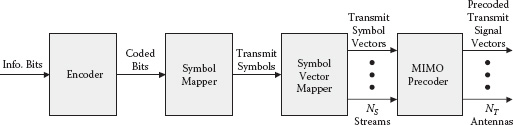
FIGURE 8.1 MIMO SM transmitter.

At the receiver side, the received signal at a given time can be represented as

$y = H x + z,$ $y = H x + z,$

(8.1)

where y = [y₁…y_NR]^T is an (N_R × 1) receive signal vector, x = [x₁…x_NS]^T is an (N_R × 1) transmit symbol vector, z is an (N_R × 1) noise vector, and H = [h₁ h₂ … h_NS] is an (N_R × N_R) effective channel matrix with h_m representing an (N_R × 1) channel gain vector from the mth stream to all receive antennas. The effective channel matrix combines the effect of the transmitter precoding and the wireless channel. The time index is omitted to simplify the notation.

In the preceding receive signal model, it was assumed that the channel is flat fading. When the channel is frequency selective, orthogonal frequency division multiplexing (OFDM) can be employed. Then, the preceding channel model still applies for each subcarrier of the OFDM system. The noise vector is an independent, identically distributed (i.i.d.) circularly symmetric complex Gaussian random vector. Without loss of generality, the variance of each element of the noise vector is set to $σ_{z}^{2} = 1$ $σ_{z}^{2} = 1$ . Then the probability density function (pdf) of the noise vector z is given as

$f (z) = \frac{1}{π^{N_{R}}} \exp (- {‖ z ‖}^{2}) .$ $f (z) = \frac{1}{π^{N_{R}}} \exp (- {‖ z ‖}^{2}) .$

(8.2)

This noise variable can be modeled to follow a Gaussian distribution with any covariance matrix after whitening and normalization. Thus, the effective channel includes the whitened noise with the transmitter precoding over wireless channels.

8.2.4 HARD-DETECTION AND SOFT-DETECTION RECEVIERS

In this subsection, hard and soft SM detection is explained with the maximum likelihood (ML) criterion and one-way connection between the detector and decoder. Figure 8.2(a) shows a MIMO receiver model with hard decoding. The MIMO hard detector estimates a transmit symbol vector from the signal vector received at the N_R receive antennas. Each element of the transmit symbol vector is demapped to the candidate symbol on the constellation used at the transmitter, and in turn the coded bits transmitted are estimated. The estimated coded bit is used by a hard decoder to generate the data bit estimates. An uncoded system can be viewed as a special case of this hard decoding, where there exists no encoder at the transmitter and no decoder at the receiver. Thus, the same MIMO hard detection can be applied to the uncoded system.

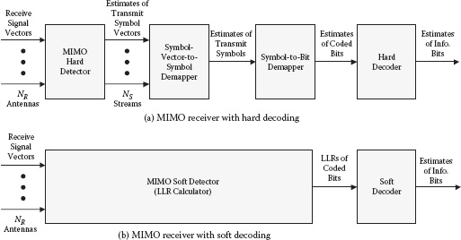
FIGURE 8.2 MIMO SM receiver.

One of the most complex parts for designing a MIMO receiver with hard decoding is a MIMO hard detector, which estimates a transmit symbol vector from a receive signal vector y. The ML estimate of the transmit symbol vector is given by

$\hat{x} = \underset{x \in X}{argmax f} (y | x),$ $\hat{x} = \underset{x \in X}{argmax f} (y | x),$

(8.3)

where X is a set of all possible M^NS transmit symbol vectors, and

$f (y | x) = \frac{1}{π^{N_{R}}} \exp (- {‖ y - H x ‖}^{2})$ $f (y | x) = \frac{1}{π^{N_{R}}} \exp (- {‖ y - H x ‖}^{2})$

(8.4)

is the conditional pdf of a receive signal vector y given a transmit symbol vector x with a known channel matrix H. From (8.3) and (8.4), the ML estimate of the transmit symbol vector can be represented as

$\hat{x} = \underset{x \in X}{argmin} ‖ y - H x ‖^{2},$ $\hat{x} = \underset{x \in X}{argmin} ‖ y - H x ‖^{2},$

(8.5)

which shows that the ML estimator is equivalent to the minimum distance estimator.

The straightforward implementation of the ML hard detector (8.5) is calculating the Euclidean distance (ED) ‖y − Hx‖² for all x ∈ X and then finding the minimum ED and the corresponding $\hat{x}$ $\hat{x}$ . However, there exist more efficient algorithms that do not require the calculation of EDs for all possible transmit symbol vectors, such as a sphere decoder with an infinite initial sphere size [20,21]. Furthermore, near-ML hard detectors also exist that further reduce the number of ED calculations [19,22,23].

Figure 8.2(b) shows a MIMO receiver model with soft decoding. In contrast to a receiver with hard decoding, the LLRs of coded bits are directly calculated from the received signal vectors. The LLR becomes an input to a soft decoder to generate the data bit estimates. The LLR for the nth bit of the sth stream, b_s,n, is

$L (b_{s, n}) = \log (\frac{P {y | b_{s, n} = 1}}{P {y | b_{s, n} = 0}}) .$ $L (b_{s, n}) = \log (\frac{P {y | b_{s, n} = 1}}{P {y | b_{s, n} = 0}}) .$

(8.6)

Using the conditional pdf in (8.4), the LLR can be represented as

$L (b_{s, n}) = \log (\sum_{x \in X_{s, n}^{(1)}} \exp (- {‖ y - H x ‖}^{2})) - \log (\sum_{x \in X_{s, n}^{(0)}} \exp (- {‖ y - H x ‖}^{2})),$ $L (b_{s, n}) = \log (\sum_{x \in X_{s, n}^{(1)}} \exp (- {‖ y - H x ‖}^{2})) - \log (\sum_{x \in X_{s, n}^{(0)}} \exp (- {‖ y - H x ‖}^{2})),$

(8.7)

where $X_{s, n}^{(b)}$ $X_{s, n}^{(b)}$ is the set of transmit symbol vectors with b_s,n = b. The sets $X_{s, n}^{(0)}$ $X_{s, n}^{(0)}$ and $X_{s, n}^{(1)}$ $X_{s, n}^{(1)}$ equally partition the set X of all possible M^NS.

The LLR can be calculated in a straightforward way by literally evaluating (8.7) using EDs for all possible transmit vectors. However, the complexity is too high to implement using the state-of-art technology. Because of the complexity, a so-called max-log approximation [19,22–26], where the logarithm of the sum of multiple exponentials is approximated to the maximum among the arguments of the exponentials, is commonly employed in practice. With the max-log approximation, the following approximate LLR can be calculated:

$\tilde{L} (b_{s, n}) ≜ min_{x \in X_{s, n}^{(0)}} {‖ y - H x ‖}^{2} - min_{x \in X_{s, n}^{(1)}} {‖ y - H x ‖}^{2}$ $\tilde{L} (b_{s, n}) ≜ min_{x \in X_{s, n}^{(0)}} {‖ y - H x ‖}^{2} - min_{x \in X_{s, n}^{(1)}} {‖ y - H x ‖}^{2}$

(8.8)

However, the complexity of this approximate LLR calculation is still quite high, and even further approximation is often taken in the literature [19,23–24,25,26].

8.3 DETECTION TECHNIQUES FOR MIMO SM

As mentioned before, the gain on the data rate over SM may not be as large in practice as promised by theory unless an intelligent receiver is employed. One of the biggest hurdles for increasing the data rate is the interference among multiple streams. Thus, in order to reap the benefits of SM fully, a receiver needs to use sophisticated techniques to mitigate the interstream interference.

A traditional approach for the interstream interference mitigation is to use MIMO equalization. Various equalizers have been developed for MIMO systems such as linear equalizer (LE) or decision feedback equalizer (DFE) with the criterion of zero-forcing (ZF) or minimum mean square error (MMSE) [16,17]. Although these equalizers are simple to implement, their performance is inferior to a maximum likelihood (ML) detector that directly estimates the transmit signal rather than tries to equalize. In spite of its superior performance, the ML detector is quite complex for implementation, particularly for soft detection. There have been some efforts for the development of ML SM soft demodulators. In Hochwald and ten Brink [19], a soft version sphere decoder has been developed by modifying the sphere decoder for hard detection. There also exist soft versions of various M- and K-best algorithms [22]. Moreover, in Barbero and Thompson [23], a list fixed-complexity sphere decoder has been proposed with the goal of regulating the implementation complexity.

In this section, various SM detection schemes will be introduced under the soft detection. Equalization-based schemes will be briefly explained first, followed by more detailed description on ML soft detection schemes that are of main interest.

8.3.1 EQUALIZATION-BASED DETECTORS

Although ML and near-ML detectors in the previous subsection provide optimal or suboptimal performance, implementation is challenging in practice, particularly for a large number of spatial streams (e.g., N_S ≥ 3) or constellation points (e.g., 64 quadrature amplitude modulation [QAM]). Thus, much simpler detectors, such as linear equalizers or ordered successive interference canceller (SIC), have been usually employed in practice.

The linear equalizers determine the transmitted vector x by compensating channel distortions as

$\begin{matrix} {\hat{x}}_{L E Q} = {[{\hat{x}}_{1} {\hat{x}}_{2} \dots {\hat{x}}_{N S}]}^{T} \\ = {[d e c ({\tilde{x}}_{1}) d e c ({\tilde{x}}_{2}) \dots d e c ({\tilde{x}}_{N S})]}^{T} \end{matrix}$ $\begin{matrix} {\hat{x}}_{L E Q} = {[{\hat{x}}_{1} {\hat{x}}_{2} \dots {\hat{x}}_{N S}]}^{T} \\ = {[d e c ({\tilde{x}}_{1}) d e c ({\tilde{x}}_{2}) \dots d e c ({\tilde{x}}_{N S})]}^{T} \end{matrix}$

(8.9)

where ${[{\tilde{x}}_{1} {\tilde{x}}_{2} \cdot \cdot \cdot {\tilde{x}}_{N S}]}^{T} = G y$ ${[{\tilde{x}}_{1} {\tilde{x}}_{2} \cdot \cdot \cdot {\tilde{x}}_{N S}]}^{T} = G y$ and $d e c ({\tilde{x}}_{s}) = (\underset{x \in Ω}{\arg \min} | x - {\tilde{x}}_{s} |)$ $d e c ({\tilde{x}}_{s}) = (\underset{x \in Ω}{\arg \min} | x - {\tilde{x}}_{s} |)$ map equalized output ${\tilde{x}}_{s}$ ${\tilde{x}}_{s}$ into the closest constellation point (i.e., slicing). Here, Ω is the set of constellation points and G is an equalizing matrix of zero-forcing (ZF), minimum mean square error (MMSE), and maximal ratio combining (MRC) linear detectors as

$G = {\begin{cases} {(H^{H} H)}^{- 1} H^{H}, ZF \\ {(H^{H} H + σ_{z}^{2} I)}^{- 1} H^{H}, MMSE \\ {(d i a g (H^{H} H))}^{- 1} H^{H}, MRC \end{cases}$ $G = {\begin{cases} {(H^{H} H)}^{- 1} H^{H}, ZF \\ {(H^{H} H + σ_{z}^{2} I)}^{- 1} H^{H}, MMSE \\ {(d i a g (H^{H} H))}^{- 1} H^{H}, MRC \end{cases}$

(8.10)

where diag(A) is matrix A with zero nondiagonals and H denotes complex conjugate.

For better performance than linear equalizers with some additional complexity, conventionally ordered (CO)-SIC can also be employed by repeatedly performing nulling and cancelling where the signals are detected according to the increasing order of the noise amplification [16]. In addition, different ordering can be used for the SIC detector considering error propagation, as in Kim and Kim [30]. After the hard decision is made, it can be used for LLR calculation as in Ketonen, Juntti, and Cavallaro [29].

8.3.2 ML TYPE DETECTION

The previously mentioned linear detectors are based on the philosophy of spatial filtering, where each of the multiplexed signal streams is separated into unique spatial dimensions at the receiver. On the other hand, the ML type detector has the capability of simultaneously identifying the spatially multiplexed signals by carrying out an exhaustive search over the legitimate signal space, providing better performance [26]. Here, more detailed explanations on ML type tree-search-based soft SM detection will be given for conventional schemes and a proposed scheme named dimension reduction soft detector (DRSD).

8.3.2.1 Conventional Near-ML Detectors

In this section, the basic principle of the conventional near-ML detectors is briefly explained. Let the MIMO detector have spatial streams of x_s in a decreasing order (i.e., from s = N_S to s = 1), without loss of generality, where a stream ordering is determined in an appropriate way [9]. For example, list fixed-complexity sphere decoder (LFSD), which provides very small and fixed implementation complexity with competitive performance, selects a stream with the smallest noise power amplification among the remaining streams to achieve the best SNR unless all the M points are chosen as candidates [31]. LFSD searches through a tree with N_s levels where k_s child nodes with the smallest d_s are retained out of M candidates from each parent node at the sth level (stream). Thus, the total number of paths in the tree from the root s = N_S to the leaves s = 1 is

$K s (= Π_{s = 1}^{N S} k_{s}) .$ $K s (= Π_{s = 1}^{N S} k_{s}) .$

Similar operations are performed in M-algorithm for candidate selection except that K_M candidates are retained at every tree level [21]. Other methods can be explained in a similar way using the tree search traversal with different symbol candidate selection [22,23,31].

Once all the K candidates are obtained (e.g., K = K_S for LFSD or K = K_M for M-algorithm), LLR can be computed based on the approximation form of (8.8) as

$\begin{array}{l} L (b_{s, n}) \approx \frac{1}{σ_{z}^{2}} [min_{x \in {\bar{X}}_{s, n}^{(0)}} {‖ y - H x ‖}^{2} - min_{x \in {\bar{X}}_{s, n}^{(1)}} {‖ y - H x ‖}^{2}] \\ = \frac{1}{σ_{z}^{2}} ({‖ y^{'} - R {\bar{x}}_{s, n}^{(0)} ‖}^{2} - {‖ y^{'} - R {\bar{x}}_{s, n}^{(1)} ‖}^{2}) \end{array}$ $\begin{array}{l} L (b_{s, n}) \approx \frac{1}{σ_{z}^{2}} [min_{x \in {\bar{X}}_{s, n}^{(0)}} {‖ y - H x ‖}^{2} - min_{x \in {\bar{X}}_{s, n}^{(1)}} {‖ y - H x ‖}^{2}] \\ = \frac{1}{σ_{z}^{2}} ({‖ y^{'} - R {\bar{x}}_{s, n}^{(0)} ‖}^{2} - {‖ y^{'} - R {\bar{x}}_{s, n}^{(1)} ‖}^{2}) \end{array}$

(8.11)

where ${\bar{X}}_{s, n}^{(b)}$ ${\bar{X}}_{s, n}^{(b)}$ is the set of transmit symbol vectors remaining after the tree search with b_s,n = b, and ${\bar{X}}_{s, n}^{(0)} \subset X_{s, n}^{(0)}, {\bar{X}}_{s, n}^{(1)} \subset X_{s, n}^{(1)} and | {\bar{X}}_{s, n}^{(0)} \cup {\bar{X}}_{s, n}^{(1)} | = K$ ${\bar{X}}_{s, n}^{(0)} \subset X_{s, n}^{(0)}, {\bar{X}}_{s, n}^{(1)} \subset X_{s, n}^{(1)} and | {\bar{X}}_{s, n}^{(0)} \cup {\bar{X}}_{s, n}^{(1)} | = K$ for s = 1,…,N_s, n = 1,…,N, and

${\bar{x}}_{s, n}^{(b)} =_{x \in {\bar{X}}_{s, n}^{(b)}}^{argmin} ‖ y - H x_{s, n}^{(b)} ‖^{2} .$ ${\bar{x}}_{s, n}^{(b)} =_{x \in {\bar{X}}_{s, n}^{(b)}}^{argmin} ‖ y - H x_{s, n}^{(b)} ‖^{2} .$

When there is no candidate in any stream, bit index, or bit value (0 or 1) (i.e., $| {\bar{X}}_{s, n}^{(0)} | = 0$ $| {\bar{X}}_{s, n}^{(0)} | = 0$ for any s, n, or b), a default value L_f may be assigned for this bit-wise element deficiency case to the LLR for the corresponding bit (i.e., L(b_{s, n}) = ± L_f), as in Wei, Rasmussen, and Wyrwas [20] and Waters and Barry [21], resulting in performance degradation. Note that the receiver performance improves as K increases since ${\bar{x}}_{s, n}^{(b)}$ ${\bar{x}}_{s, n}^{(b)}$ is more likely to exist in the final candidate set ${\bar{X}}_{s, n}^{(b)}$ ${\bar{X}}_{s, n}^{(b)}$ and thus the use of the default value can be avoided. However, large K increases the computation burden since more candidates have to be compared to find ${\bar{x}}_{s, n}^{(b)}$ ${\bar{x}}_{s, n}^{(b)}$

8.3.2.2 Dimension Reduction Soft Detector

In this section, a recently proposed SM soft demodulator that utilizes existing hard detectors directly is introduced [28]. It can be noted that the conventional near-ML approach was to consider all transmit symbol values for all streams at the same time exhaustively. On the other hand, the equalizer-based approach that was described before does not consider any stream for exhaustive ED calculation and put all the computational burden to hard detection. A good mix of these two approaches is to consider partial numbers of streams for exhaustive ED calculation and rely on hard detectors to find the best transmit symbol subvector for the remaining streams.

First, the problem of calculating the LLRs for part of N_S streams is investigated in detail. The problem of calculating the LLRs for all N_S streams is addressed later in this section. Let $N_{S}^{s o}$ $N_{S}^{s o}$ be the number of streams on which soft demodulation will be performed, and let $N_{S}^{h a}$ $N_{S}^{h a}$ be the number of remaining streams (i.e., $N_{S}^{h a} = N s - N_{S}^{s o}$ $N_{S}^{h a} = N s - N_{S}^{s o}$ ). Let x^so be the transmit symbol subvector corresponding to soft demodulation streams, and x^ha be the transmit symbol subvector corresponding to the remaining streams. Finally, a rearranged transmit symbol vector can be formed by stacking x^ha on top of x^so:

$\tilde{x} = [_{x^{s o}}^{x^{h a}}]$ $\tilde{x} = [_{x^{s o}}^{x^{h a}}]$

(8.12)

For example, consider the case of demodulating the first stream and the third stream softly out of N_S = 4 streams. Then, $N_{S}^{s o} = 2, x^{s o} = {[x_{1} x_{3}]}^{T}, x^{h a} = {[x_{2} x_{4}]}^{T} and \tilde{x} = [x_{2} x_{4} x_{1} x_{3}]$ $N_{S}^{s o} = 2, x^{s o} = {[x_{1} x_{3}]}^{T}, x^{h a} = {[x_{2} x_{4}]}^{T} and \tilde{x} = [x_{2} x_{4} x_{1} x_{3}]$ .

The rearranged transmit symbol vector $\tilde{x}$ $\tilde{x}$ can be represented using some permutation matrix P as follows:

$\tilde{x} ≜ P x,$ $\tilde{x} ≜ P x,$

(8.13)

where permutation matrix P is, by definition, a square matrix that has exactly one entry with a value of 1 in each row and each column and all the other entries with a value of 0. Similarly, the columns of the channel matrix are rearranged using the permutation matrix P:

$\tilde{H} ≜ H P^{T} = [H^{^{h a}} H^{^{s o}}],$ $\tilde{H} ≜ H P^{T} = [H^{^{h a}} H^{^{s o}}],$

(8.14)

where $H^{^{s o}} \in C^{N_{R} \times N_{S}^{s o}}$ $H^{^{s o}} \in C^{N_{R} \times N_{S}^{s o}}$ and $H^{^{h a}} \in C^{N_{R} \times N_{S}^{h a}}$ $H^{^{h a}} \in C^{N_{R} \times N_{S}^{h a}}$ represent the channel submatrices for the soft-demodulation streams x^so and the remaining streams x^ha.

With the preceding permutation on the transmit symbol vector and the channel matrix, the received signal can be represented as

$\begin{array}{l} y = H x + z \\ = \tilde{H} \tilde{x} + z \\ = H^{h a} x^{h a} + H^{s o} x^{s o} + z . \end{array}$ $\begin{array}{l} y = H x + z \\ = \tilde{H} \tilde{x} + z \\ = H^{h a} x^{h a} + H^{s o} x^{s o} + z . \end{array}$

(8.15)

The second equality holds because $\tilde{H} \tilde{x} = (H P^{T}) (P x) = H (P^{T} P) x = H x$ $\tilde{H} \tilde{x} = (H P^{T}) (P x) = H (P^{T} P) x = H x$ , which uses a basic permutation matrix property that the inverse of a permutation matrix is the transpose of the permutation matrix.

Then the LLR for the nth bit of the sth stream is

$\tilde{L} (b_{s, n}) = \min_{x^{so} \in X_{s, n}^{s o, (0)}, x^{ha} \in X^{h a}} {‖ y - Η^{h a} x^{h a} - Η^{s o} x^{s o} ‖}^{2} - \min_{x^{so} \in X_{s, n}^{s o, (1)}, x^{ha} \in X^{h a}} {‖ y - Η^{h a} x^{h a} - Η^{s o} x^{s o} ‖}^{2}$ $\tilde{L} (b_{s, n}) = \min_{x^{so} \in X_{s, n}^{s o, (0)}, x^{ha} \in X^{h a}} {‖ y - Η^{h a} x^{h a} - Η^{s o} x^{s o} ‖}^{2} - \min_{x^{so} \in X_{s, n}^{s o, (1)}, x^{ha} \in X^{h a}} {‖ y - Η^{h a} x^{h a} - Η^{s o} x^{s o} ‖}^{2}$

(8.16)

where $X_{s, n}^{s o, (b)}$ $X_{s, n}^{s o, (b)}$ is the set of soft-demodulation transmit symbol subvectors x^so with b_s,n = b, and X^ha is the set of all hard-detection transmit symbol subvectors x^ha. The implicit assumption in the preceding LLR expression is that the sth stream belongs to the set of soft-demodulation streams. Calculating the minimum ED over the sets $X_{s, n}^{s o, (b)}$ $X_{s, n}^{s o, (b)}$ and X^ha can be performed in two steps: Calculate the minimum ED over the set X^ha for each x^so and then take the minimum ED among all soft-demodulation transmit symbol subvectors in $X_{s, n}^{s o, (b)}$ $X_{s, n}^{s o, (b)}$ . Thus, the LLR can be represented as

$\tilde{L} (b_{s, n}) = \min_{x^{so} \in X_{s, n}^{s o, (0)}} (\min_{x^{ha} \in X^{h a}} {‖ y^{h a} (x^{s o}) - Η^{h a} x^{h a} ‖}^{2}) - \min_{x^{so} \in X_{s, n}^{s o, (1)}} (\min_{x^{ha} \in X^{h a}} {‖ y^{h a} (x^{s o}) - Η^{h a} x^{h a} ‖}^{2})$ $\tilde{L} (b_{s, n}) = \min_{x^{so} \in X_{s, n}^{s o, (0)}} (\min_{x^{ha} \in X^{h a}} {‖ y^{h a} (x^{s o}) - Η^{h a} x^{h a} ‖}^{2}) - \min_{x^{so} \in X_{s, n}^{s o, (1)}} (\min_{x^{ha} \in X^{h a}} {‖ y^{h a} (x^{s o}) - Η^{h a} x^{h a} ‖}^{2})$

(8.17)

where

$y^{h a} (x^{s o}) ≜ y - H^{s o} x^{s o},$ $y^{h a} (x^{s o}) ≜ y - H^{s o} x^{s o},$

(8.18)

which is formed by subtracting the influence of the transmit symbol subvector x^so from the received signal.

A MIMO ML hard detector efficiently finds the transmit symbol vector ${\hat{x}}^{h a} (x^{s o})$ ${\hat{x}}^{h a} (x^{s o})$ that minimizes ED:

${\hat{x}}^{h a} (x^{s o}) = \underset{x^{ha} \in X^{h a}}{argmin} {‖ y^{h a} (x^{s o}) - H^{h a} x^{h a} ‖}^{2} .$ ${\hat{x}}^{h a} (x^{s o}) = \underset{x^{ha} \in X^{h a}}{argmin} {‖ y^{h a} (x^{s o}) - H^{h a} x^{h a} ‖}^{2} .$

(8.19)

The corresponding minimum ED is calculated as follows:

$D (x^{s o}) = {‖ y^{h a} (x^{s o}) - H^{h a} {\hat{x}}^{h a} (x^{s o}) ‖}^{2} .$ $D (x^{s o}) = {‖ y^{h a} (x^{s o}) - H^{h a} {\hat{x}}^{h a} (x^{s o}) ‖}^{2} .$

(8.20)

Then, the LLR can be calculated using the following equation:

$\tilde{L} (b_{s, n}) = \min_{x^{so} \in X_{s, n}^{s o, (0)}} D (x^{s o}) - \min_{x^{so} \in X_{s, n}^{s o, (1)}} D (x^{s o}) .$ $\tilde{L} (b_{s, n}) = \min_{x^{so} \in X_{s, n}^{s o, (0)}} D (x^{s o}) - \min_{x^{so} \in X_{s, n}^{s o, (1)}} D (x^{s o}) .$

(8.21)

When LLR needs to be calculated for all streams, the preceding LLR calculation can be performed multiple times with different permutation matrices such that each stream belongs to soft-demodulation streams at least once. Partitioning the streams into soft-demodulation streams can be performed in many different ways. For example, when the total number of streams is four, then the soft-demodulation dimension can be chosen as one such that the partial LLR calculation is performed four times. Another option is to choose the soft-demodulation dimension as two such that the partial LLR calculation is performed twice.

Figure 8.3 shows a block diagram of the partial demodulator with the proposed dimension reduction approach. The first block is a candidate subset generation block for soft-demodulation transmit symbol subvectors. The second block forms a new received signal vector that removes the effect of the soft-demodulation transmit symbol subvectors from the original received signal vector. Then, a hard-detection problem is solved with the dimension of $N_{S}^{h a}$ $N_{S}^{h a}$ in the third block. In the following block, based on the estimate of the hard-detection transmit symbol subvector, ED for each soft-demodulation transmit symbol subvector is calculated. Lastly, the LLR is calculated based on the EDs. More details on the DRSD including the comparison of the performance and complexity with other conventional schemes are available in Lee, Choi, and Lou [28].

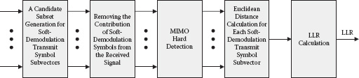
FIGURE 8.3 Partial MIMO soft demodulator with dimension reduction approach.

8.3.2.2.1 Performance and Complexity of DRSD

In this section, the complexity of the proposed DRSD is evaluated first. As a complexity measure, the number of visited nodes is chosen when QR decomposition is used and the demodulation problem is formulated as a tree search problem. With the use of QR decomposition, ED can be computed recursively from s = N_S to s = 1 based on

${‖ w - R x ‖}^{2} = \sum_{j = 1}^{N_{S}} {(w_{j} - \sum_{i = j}^{N_{S}} r_{j i} x_{i})}^{2}$ ${‖ w - R x ‖}^{2} = \sum_{j = 1}^{N_{S}} {(w_{j} - \sum_{i = j}^{N_{S}} r_{j i} x_{i})}^{2}$

(8.22)

where H = QR, y′ = Q^Hy, Q is an (N_R × N_R) unitary matrix, and R is an (N_R × N_S) upper triangular matrix; r_ji denotes the entry in the jth row and the ith column of R. This ED calculation can be represented as a tree structure where layer 1 has M nodes representing M different values of x_NS and each node in layer i has M children nodes in layer i + 1 with M different values of x_NS-i for 1 ≤ i ≤ N_S – 1. With this complexity measure, it is inherently assumed that the complexity associated with each node in a tree is the same regardless of the node location. Although the actual number of operations per node can vary depending on the node location, choosing the number of operations as the complexity measure makes the analysis too complicated. Thus, in this section, the number of visited nodes has been chosen as the complexity measure (see Jalden and Ottersten [31]).

With the conventional exhaustive search method, the number of visited nodes is

$C_{e x h} (N_{S}) = \sum_{i = 1}^{N_{S}} M^{i} = \frac{M (M^{N_{S}} - 1)}{M - 1},$ $C_{e x h} (N_{S}) = \sum_{i = 1}^{N_{S}} M^{i} = \frac{M (M^{N_{S}} - 1)}{M - 1},$

(8.23)

since the exhaustive search visits all the nodes of the tree that has Mⁱ nodes in layer i for i = 1, 2, …,N_S. With the near-exhaustive search method in Lee et al. [32] that reduces the computation at the final stream, the number of visited nodes is

$\begin{array}{l} C_{n e a r - e x h} (N_{S}) = \sum_{i = 1}^{N_{S} - 1} M^{i} + (1 + \log_{2} M) M^{N_{S} - 1} \\ = \frac{M (M^{N_{S} - 1} - 1)}{M - 1} + (1 + \log_{2} M) M^{N_{S} - 1} \end{array}$ $\begin{array}{l} C_{n e a r - e x h} (N_{S}) = \sum_{i = 1}^{N_{S} - 1} M^{i} + (1 + \log_{2} M) M^{N_{S} - 1} \\ = \frac{M (M^{N_{S} - 1} - 1)}{M - 1} + (1 + \log_{2} M) M^{N_{S} - 1} \end{array}$

(8.24)

because only (1+ log₂ M)M^NS-1 nodes out of M^NS nodes in layer N_S need to be visited.

On the other hand, the number of visited nodes for the soft demodulation of $N_{S}^{s o}$ $N_{S}^{s o}$ streams using the DRSD is

$C_{D R S D, p a r t} (N_{S}, N_{S}^{s o}) = \frac{M (M^{N_{s}^{s o}} - 1)}{M - 1} + M^{N_{S}^{s o}} C_{h a r d} (N_{s} - N_{S}^{s o})$ $C_{D R S D, p a r t} (N_{S}, N_{S}^{s o}) = \frac{M (M^{N_{s}^{s o}} - 1)}{M - 1} + M^{N_{S}^{s o}} C_{h a r d} (N_{s} - N_{S}^{s o})$

(8.25)

where $C_{h a r d} (N)$ $C_{h a r d} (N)$ is the number of visited nodes of the considered hard detector with N streams. This number of visited nodes can be derived by noting that all the nodes in layer 1 to layer $N_{S}^{s o}$ $N_{S}^{s o}$ are visited and the number of visited nodes in layers s > $N_{S}^{s o}$ $N_{S}^{s o}$ depends on the hard detector.

When $N_{S}^{s o}$ $N_{S}^{s o}$ streams are demodulated softly at one time and the same partial demodulator is used multiple times with reordering of streams, the partial demodulator should be used $⌈ N_{s} / N_{S}^{s o} ⌉$ $⌈ N_{s} / N_{S}^{s o} ⌉$ times, where ⎡x⎤ represents the ceiling operation (i.e., it is the smallest integer that is not less than x). For example, when three streams are demodulated at the same time out of a total of five streams, the partial demodulator needs to be used twice, such as x^so = [x₁ x₂ x₃]^T for the first time and x^so = [x₄ x₅ x₁]^T for the second time. In this case, the LLR for x₁ is calculated twice. With the repeated use of the same partial DRSD $⌈ N_{s} / N_{S}^{s o} ⌉$ $⌈ N_{s} / N_{S}^{s o} ⌉$ times, the total number of visited nodes for the demodulation of all N_S streams is

$C_{D R S D, t o t} (N_{S}, N_{S}^{s o}) = ⌈ N_{s} / N_{S}^{s o} ⌉ C_{D R S D, p a r t} (N_{S}, N_{S}^{s o})$ $C_{D R S D, t o t} (N_{S}, N_{S}^{s o}) = ⌈ N_{s} / N_{S}^{s o} ⌉ C_{D R S D, p a r t} (N_{S}, N_{S}^{s o})$

(8.26)

When a different partial demodulator is allowed to be used each time, the total number of ED can be expressed as

$C_{D R S D, t o t} = \sum_{p = 1}^{P} M^{N_{S, p}^{s o}} C_{D R S D, p a r t} (N_{S}, N_{S} - N_{S, p}^{s o}) .$ $C_{D R S D, t o t} = \sum_{p = 1}^{P} M^{N_{S, p}^{s o}} C_{D R S D, p a r t} (N_{S}, N_{S} - N_{S, p}^{s o}) .$

(8.27)

The optimality of the proposed DRSD can be maintained by the use of the optimal hard detector. However, by sacrificing the optimality, further reduction in complexity can be achieved—that is, lower $C_{h a r d} (N)$ $C_{h a r d} (N)$ . One easy way of reducing complexity is using a suboptimal hard detector such as numerous existing near-ML hard detectors, linear equalizers, and decision feedback equalizers. The use of suboptimal hard detectors may cause significant performance loss. In this case, as a compromise of complexity and performance, multiple suboptimal hard detectors can be used instead of one suboptimal hard detector [35]. Another way of reducing complexity is considering less than $M^{N_{S}^{s o}}$ $M^{N_{S}^{s o}}$ candidates for soft-demodulation transmit symbol subvectors [36].

To see the performance of the DRSD scheme, simulation results of the optimal DRSD and low complexity DRSDs are given in the setting of WiMAX radio conformance tests [33] (RCT) for IEEE 802.16-based systems [34]. For the low complexity DRSDs, suboptimal hard detectors are considered. Orthogonal frequency division multiple access (OFDMA) modes in IEEE 802.16 are chosen for the simulation. With the OFDMA mode, a convolutional turbo code (CTC) is used for channel coding along with the bit-interleaved coded modulation (BICM), and MIMO soft demodulation is performed subcarrier by subcarrier. Among the various channel models defined in WiMAX RCT, a vehicular-A 60 km/h channel is chosen for the determination of the power delay profile and the Doppler spread of the multipath fading channel. For antenna correlation, both the low and high correlation models of WiMAX RCT are considered.

Figure 8.4(a) shows packet error rate (PER) curves for various soft demodulators for 4 QAM and coding rate of 1/2 with four transmit and four receive antennas having the high spatial correlation. Here, four streams are transmitted, and the number of soft demodulation streams is chosen as one for the DRSD. As can be seen in the figure, the suboptimal DRSD that uses multiple SIC hard detectors with all possible detection orders [35] (represented as “mixed SIC” in the figure) as a suboptimum hard detector shows little performance loss compared to the optimal soft demodulator. The suboptimal DRSD based on ordered SIC [22] shows some performance degradation of approximately 0.7 dB at 10% PER but still outperforms MMSE LE by approximately 1.7 dB. In Figure 8.4(b), PER curves for 16 QAM and coding rate of 1/2 are shown when the other simulation parameters are the same as in Figure 8.4(a). Figure 8.4(b) exhibits similar trends as Figure 8.4(a) but with more pronounced differences among the soft demodulators at 10% PER. Similar tendencies can be observed for spatially low correlated channels. More evaluation results for the performance and complexity can be obtained in Lee et al. [28].

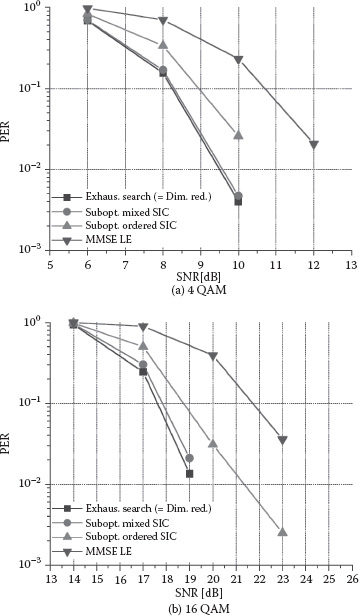
FIGURE 8.4 PER curves with four transmit and four receive antennas.

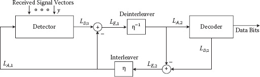
FIGURE 8.5 A block diagram of iterative detecting and decoding receiver

8.4 ITERATIVE DETECTION AND DECODING

The iterative detection and decoding (IDD) scheme exploits the feedback path from the decoder to the detector [19]. The IDD scheme iteratively exchanges soft information between the detector and the decoder in a two-way algorithm as shown in Figure 8.5. Even though the IDD scheme is not strictly proved as an optimal algorithm, it is very effective to decode the symbol and to achieve the near-optimal result. Under the IDD scheme, the kind of LLR is divided into three types: a priori LLR, extrinsic LLR, and a posteriori LLR. The output of a detector or a decoder denotes a posteriori LLR that is generated by using the input, a priori LLR. Therefore, only the extrinsic LLR obtained by subtracting a priori LLR from a posteriori LLR is exchanged between the detector and the decoder. While iterating to detect and decode the receive signal, a posteriori LLR becomes accurate and correspondingly more accurate a priori LLR can be used to detect and decode. The iterating process continues until the stopping criterion is satisfied or the improvement over the IDD scheme is negligible.

8.4.1 SYSTEM MODEL

As introduced in Hochwald and ten Brink [19], the IDD architecture is designed with both the detector and the decoder, and the set of an interleaver and a deinterleaver on the path where the soft information is exchanged. As these authors explain [19], the IDD scheme can be introduced from the received signal y as

$y = H x + z$ $y = H x + z$

(8.28)

where H is a complex channel matrix whose dimension is the number of receiver antennas, N_R, times the number of spatial streams N_S. In general, N_R and N_S are not restricted to one such that the detector can be extended to the MIMO detector explained in the previous section. The noise z is a vector whose element follows an independent complex Gaussian distribution with mean zero. The signal vector x has its elements as discrete modulated symbols with energy constraint as

$x = [\begin{matrix} x_{1} \\ \cdot \\ \cdot \\ \cdot \\ x_{N S} \end{matrix}],$ $x = [\begin{matrix} x_{1} \\ \cdot \\ \cdot \\ \cdot \\ x_{N S} \end{matrix}],$

(8.29)

where x_i is the ith element of x. It is noted that a symbol consists of N bits and, correspondingly, a signal vector consists of N_SN bits. In particular, the nth bit of the sth stream is expressed as b_s,n. Thus, using any of the detection algorithms such as MAP detecting, the signal vector could be estimated and the estimated signal symbols associated with a single codeword could be collected accordingly. The estimated symbols are equivalently transformed into the soft bit information and passed to the decoder as extrinsic LLRs.

8.4.2 SOFT INFORMATION

In detail, the soft information obtained from the detector can be explained [19] as follows. Given the received signal y, the a posteriori LLR of the bit b_s,n is

$\begin{array}{l} L_{D} (b_{s, n} | y) = \ln \frac{P (b_{s, n} = + 1 | y)}{P (b_{s, n} = - 1 | y)}, \end{array}$ $\begin{array}{l} L_{D} (b_{s, n} | y) = \ln \frac{P (b_{s, n} = + 1 | y)}{P (b_{s, n} = - 1 | y)}, \end{array}$

(8.30)

where the subscript D stands for a posteriori LLR. Under the assumption that the interleaver provides fully independent output bits after scrambling input bits, each bit b_s,n is considered statistically independent of neighbor bits. Then, using Bayes’s theorem, the a posteriori LLR can be divided into the sum of a priori LLR, L_A, and the extrinsic LLR, L_E, as

$\begin{array}{l} L_{D} (b_{s, n} | y) = L_{A} (b_{s, n}) + \ln \frac{\sum_{b \in β_{s, n + 1}} P (y | b) (\exp \sum_{(i, j) \in ϑ_{s, n + 1}} L_{A} (b_{i, j}))}{\sum_{b \in β_{s, n - 1}} P (y | b) (\exp \sum_{(i, j) \in ϑ_{s, n - 1}} L_{A} (b_{i, j}))} \\ = L_{A} (b_{s, n}) + L_{E} (b_{s, n} | y) \end{array}$ $\begin{array}{l} L_{D} (b_{s, n} | y) = L_{A} (b_{s, n}) + \ln \frac{\sum_{b \in β_{s, n + 1}} P (y | b) (\exp \sum_{(i, j) \in ϑ_{s, n + 1}} L_{A} (b_{i, j}))}{\sum_{b \in β_{s, n - 1}} P (y | b) (\exp \sum_{(i, j) \in ϑ_{s, n - 1}} L_{A} (b_{i, j}))} \\ = L_{A} (b_{s, n}) + L_{E} (b_{s, n} | y) \end{array}$

(8.31)

where the set β_s,n,+1 is defined as

$β_{s, n + 1} = {b | b_{s, n} = + 1}$ $β_{s, n + 1} = {b | b_{s, n} = + 1}$

(8.32)

$β_{s, n + 1} = {b | b_{s, n} = - 1} .$ $β_{s, n + 1} = {b | b_{s, n} = - 1} .$

(8.33)

The bit vector b indicates the concatenated bits of x in a vector form. Also, the set ϑ_s,nb is given by

$ϑ_{s, n, k} = {(i, j) | i = 1, …, N_{s}, j = 1, …, N, (i, j) \neq (s, n), b_{(i, j)} = k}, k = + 1 or - 1 .$ $ϑ_{s, n, k} = {(i, j) | i = 1, …, N_{s}, j = 1, …, N, (i, j) \neq (s, n), b_{(i, j)} = k}, k = + 1 or - 1 .$

(8.34)

The a priori LLR is defined as the ratio of the bit probability and is expressed as

$L_{A} (b_{k}) = \ln \frac{P (b_{s, n} = + 1)}{P (b_{s, n} = - 1)} .$ $L_{A} (b_{k}) = \ln \frac{P (b_{s, n} = + 1)}{P (b_{s, n} = - 1)} .$

(8.35)

The conditional probability P(y | b) depends on the detector. For the case of the MAP detector, the conditional probability is a function of exponential terms. As explained in Hochwald and ten Brink [19], the extrinsic LLR is converted by multiplying the constant

$\sum_{s} \sum_{n} L_{A} (b_{s, n})$ $\sum_{s} \sum_{n} L_{A} (b_{s, n})$

into the following:

$L_{D} (b_{s, n} | y) = \ln \frac{\underset{b \in β_{s, n + 1}}{\sum^{}} P (y | b) \exp (\frac{1}{2} b_{[s, n]}^{†} L_{A,}_{[s, n]})}{\underset{b \in β_{s, n - 1}}{\sum^{}} P (y | b) \exp (\frac{1}{2} b_{[s, n]}^{†} L_{A,}_{[s, n]})},$ $L_{D} (b_{s, n} | y) = \ln \frac{\underset{b \in β_{s, n + 1}}{\sum^{}} P (y | b) \exp (\frac{1}{2} b_{[s, n]}^{†} L_{A,}_{[s, n]})}{\underset{b \in β_{s, n - 1}}{\sum^{}} P (y | b) \exp (\frac{1}{2} b_{[s, n]}^{†} L_{A,}_{[s, n]})},$

(8.36)

where the subscript [s, n] denotes that the nth bit of the s-stream is excluded in the vector associated with the subscript. The extrinsic LLR is interpreted as the soft information of each bit so as to be passed to the decoder. Figure 8.5 depicts a block diagram of the IDD receiver in detail. The subscript 1 attached in the L-values implies that the L-values work for the detector. On the other hand, the subscript 2 denotes that the L-values are with the decoder. As shown in Figure 8.5, the decoder output is treated in the same way as the detector output; that is, a priori LLR of the decoder is subtracted from the decoder output, a posteriori LLR, and the resultant extrinsic LLR is fed back to the detector after being descrambled at the deinterleaver. This process is iteratively repeated until the decoding performance or the stopping criterion is satisfied.

Figure 8.6(a) and (b) shows PER of the IDD receiver using a MAP detector and a turbo decoder in terms of the number of iterations between the detector and the decoder. The 4 × 4 MIMO channel is considered with two code words such that one codeword is assigned over two layers. The turbo code is generated with the polynomial (7, 5) and two code rates, 0.33 and 0.83. It is observed that the PER curves quickly drop as the number of iterations between the detector and the decoder increases. Since the bit sequence having a low code rate is encoded with more redundancy, the PER slope of the corresponding bit sequence is shown to be much more rapid. Also, when the number of iterations is large enough, the updated LLRs from the IDD receiver become accurate, so the PER is also saturated. In this case, no more gain is achieved.

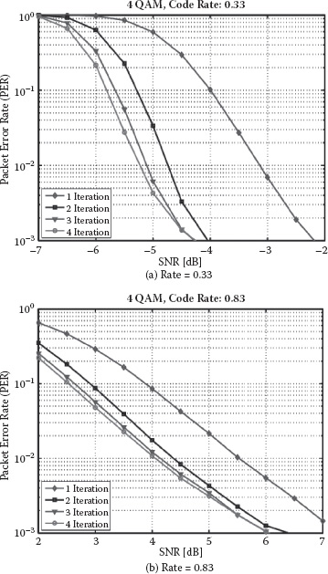
FIGURE 8.6 The PER of a 4 × 4 IDD receiver using a MAP detector and a turbo decoder with 4 QAM.

8.5 CONCLUSIONS AND FUTURE DIRECTIONS

In this chapter, we examined various MIMO SM receiver schemes. We provided a comprehensive review of conventional detectors as well as advanced detectors for both hard and soft decoding. In particular, we presented a dimension reduction soft detector for soft decoding that achieves near-ML performance at a low complexity. We also described an iterative detection and decoding architecture as an advanced receive technique to achieve the performance promised by MIMO SM. In real-world communication systems, many antennas have been adopted to meet the peak throughput requirement. Therefore, it is vital to continue to develop a receiver that obtains the best trade-off between performance and complexity.

REFERENCES

1. I. E. Telatar, Capacity of multi-antenna Gaussian channels. European Transactions on Telecommunications, vol. 10, pp. 585–595, 1999.

2. Q. Li, G. Li, W. Lee, M. Lee, D. Mazzarese, B. Clerckx, and Z. Li, MIMO techniques in WiMAX and LTE: A feature overview. IEEE Communications Magazine, vol. 48, no. 5, pp. 86–92, 2010.

3. ITU-R Rep. M.2134, Requirements related to technical system performance for IMT-Advanced radio interface(s), Nov. 2008.

4. ITU-R Rec. M.1457-8, Detailed specifications of the radio interfaces of international mobile telecommunications-2000 (IMT-2000), May 2009.

5. ITU-R SG WP 5D, Acknowledgment of candidate submission from IEEE under step 3 of the IMT-advanced process (IEEE Technology), Doc. IMT-ADV/4-E, Oct. 2009.

6. ITU-R SG WP 5D, Acknowledgment of candidate submission from 3GPP proponent (3GPP Organization Partners of ARIB, ATIS, CCSA, ETSI, TTA AND TTC) under step 3 of the IMT-advanced process (3GPP Technology), Doc. IMT-ADV/8-E, Oct. 2009.

7. 3GPP TS 36.101, Evolved universal terrestrial radio access (E-UTRA); user equipment (UE) radio transmission and reception (Rel. 8), March 2010.

8. G. Heirtz, D. Denteneer, L. Stibor, Y. Zhang, X. P. Costa, and B. Walke, The IEEE 802.11 universe. IEEE Communications Magazine, vol. 48, pp. 62–70, Jan. 2010.

9. S. Yong, P. Xia, and A. Valdes-Garcia. 60 GHz Technology for Gbps WLAN and WPAN: From theory to practice. New York: Wiley, 2011.

10. X. Zhu, A. Doufexi, and T. Kocak, Throughput and coverage performance for IEEE 802.11ad millimeter-wave WPANs. Proceedings of IEEE Vehicular Technology Conference (VTC), pp. 1–5, May 2011.

11. F. Akyildiz, D. M. Gutierrez-Estevez, and E. C. Reyes, The evolution to 4G cellular systems: LTE-Advanced. Physical Communication, vol. 3, no. 4, pp 217–244, Dec. 2010.

12. S. Sugiura, S. Chen, and L. Hanzo, A universal space-time architecture for multiple-antenna-aided systems. IEEE Communications Surveys & Tutorials, vol. 14, pp. 401–420, 2012.

13. L. J. Cimini, Jr., and N. R. Sollenberger, OFDM with diversity and coding for high-bit-rate mobile data applications. Mobile Multimedia Communication, vol. 1, pp. 247–254, 1997.

14. S. M. Alamouti, A simple transmit diversity technique for wireless communications. IEEE Journal on Selected Areas in Communications, vol. 16, pp. 1451–1458, Oct. 1998.

15. G. J. Foschini, Space-time block codes from orthogonal designs. Bell Labs Technical Journal, vol. 2, pp. 41–59, 1996.

16. P. Wolniansky, G. Foschini, G. Golden, and R. Valenzuela, V-BLAST: An architecture for realizing very high data rates over the rich-scattering wireless channel. Proceedings of URSI International Symposium on Signals, Systems, and Electronics (ISSSE), pp. 295–300, Sept. 1998.

17. G. Caire, G. Taricco, and E. Biglieri, Bit-interleaved coded modulation. IEEE Transactions on Information Theory, vol. 44, no. 3, pp. 927–946, May 1998.

18. J. Hagenauer, E. Offer, and L. Papke, Iterative decoding of binary block and convolutional codes. IEEE Transactions on Information Theory, vol. 42, no. 2, pp. 429–445, March 1996.

19. B. M. Hochwald and S. ten Brink, Achieving near-capacity on a multiple-antenna channel. IEEE Transactions on Communications, vol. 51, pp. 389–399, March 2003.

20. L. Wei, L. K. Rasmussen, and R. Wyrwas, Near optimum tree-search detection schemes for bit-synchronous multiuser CDMA systems over Gaussian and two-path Rayleigh-fading channels. IEEE Transactions on Communications, vol. 45, pp. 691–700, June 1997.

21. D. W. Waters and J. R. Barry, The chase family of detection algorithms for multiple-input multiple-output channels. IEEE Transactions on Signal Processing, vol. 56, pp. 739–747, Feb. 2008.

22. Y. L. C. de Jong, and T. J. Willink, Iterative tree search detection for MIMO wireless systems. IEEE Transactions on Communications, vol. 53, pp. 930–935, June 2005.

23. L. G. Barbero and J. S. Thompson, Extending a fixed-complexity sphere decoder to obtain likelihood information for turbo-MIMO systems. IEEE Transactions on Vehicular Technology, vol. 57, pp. 2804–2814, Sept. 2008.

24. C. Studer, A. Burg, and H. Bölcskei, Soft-output sphere decoding: algorithms and VLSI implementation. IEEE Journal on Selected Areas in Communications, vol. 26, no. 2, pp. 290–300, Feb. 2008.

25. L. Milliner, E. Zimmermann, J. R. Barry, and G. Fettweis, A fixed-complexity smart candidate adding algorithm for soft-output MIMO detection. IEEE Journal on Selected Topics in Signal Processing, vol. 3, pp. 1016–1025, Dec. 2009.

26. J.-S. Kim, S.-H. Moon, and I. Lee, A new reduced complexity ML detection scheme for MIMO systems. IEEE Transactions on Communications, vol. 58, pp. 1302–1310, April 2010.

27. J. M. Cioffi and G. D. Forney, Generalized decision-feedback equalization for packet transmission with ISI and Gaussian noise. In Communication, computation, control and signal processing, ed. A. Paulraj, V. Roychowdhury, and C. Schaper. Boston: Kluwer, pp. 79–127, 1997.

28. J. Lee, J.-W. Choi, and H.-L. Lou, MIMO maximum likelihood soft demodulation based on dimension reduction. Proceedings IEEE Global Telecommunications Conference (GLOBECOM), pp. 1–5, Dec. 2010.

29. J. Ketonen, M. Juntti, and J. R. Cavallaro, Performance-complexity comparison of receivers for a LTE MIMO–OFDM system. IEEE Transactions on Signal Processing, vol. 58, no. 6, pp. 3360–3372, June 2010.

30. S. W. Kim and K. P. Kim, Log-likelihood-ratio-based detection ordering in V-BLAST. IEEE Transactions on Communications, vol. 54, pp. 302–307, Feb. 2006.

31. J. Jalden, and B. Ottersten, On the complexity of sphere decoding in digital communications. IEEE Transactions on Signal Processing, vol. 53, pp. 1474–1484, April 2005.

32. J. Lee, J.-W. Choi, H. Lou, and J. Park, Soft MIMO ML demodulation based on bitwise constellation partitioning. IEEE Communications Letters, vol. 13, pp. 736–738, Oct. 2009.

33. WiMAX forum mobile radio conformance tests (MRCT) release 1.0. (http://www.wimaxforum.org).

34. IEEE Std 802.16-2009, IEEE standard for local and metropolitan area networks, part 16: Air interface for broadband wireless access systems. IEEE, May 2009.

35. J.-W. Choi, J. Lee, H.-L. Lou, and J. Park, Improved MIMO SIC detection exploiting ML criterion. Proceedings IEEE Vehicular Technology Conference (VTC), pp. 1–5, Sept. 2011.

36. J.-W. Choi, J. Lee, J. P. Choi, and H.-L. Lou, MIMO soft near-ML demodulation with fixed low-complexity candidate selection. To be published, IEICE Transactions on Communications, vol. E-95B. pp. 2884–2891. Sept. 2012.

..................Content has been hidden....................

You can't read the all page of ebook, please click here login for view all page.

Table of Contents for Chapter 8 Efficient MIMO Receiver Design for Next Generation Wireless Systems

Create new playlist

Sign In

Sign Up

Table of Contents for
Chapter 8 Efficient MIMO Receiver Design for Next Generation Wireless Systems