4
Learning Object Pose Detection and Tracking by Differentiable Rendering
In this chapter, we are going to explore an object pose detection and tracking project by using differentiable rendering. In object pose detection, we are interested in detecting the orientation and location of a certain object. For example, we may be given the camera model and object mesh model and need to estimate the object orientation and position from one image of the object. In the approach in this chapter, we are going to formulate such a pose estimation problem as an optimization problem, where the object pose is fitted to the image observation.
The same approach as the aforementioned can also be used for object pose tracking, where we have already estimated the object pose in the 1, 2,…, up to t-1 time slots and want to estimate the object pose at the t time slot, based on one image observation of the object at t time.
One important technique we will use in this chapter is called differentiable rendering, a super-exciting topic currently explored in deep learning. For example, the CVPR 2021 Best Paper Award winner GIRAFFE: representing scenes as compositional generative neural feature fields uses differentiable rendering as one important component in its pipeline.
Rendering is the process of projecting 3D physical models (a mesh model for the object, or a camera model) into 2D images. It is an imitation of the physical process of image formation. Many 3D computer vision tasks can be considered as an inverse of the rendering process – that is, in many computer vision problems, we want to start from 2D images to estimate the 3D physical models (meshes, point cloud segmentation, object poses, or camera positions).
Thus, a very natural idea that has been discussed in the computer vision community for several decades is that we can formulate many 3D computer vision problems as optimization problems, where the optimization variables are the 3D models (meshes, or point cloud voxels), and the objective functions are certain similarity measures between the rendered images and the observed images.
To efficiently solve such an optimization problem as the aforementioned, the rendering process should be differentiable. For example, if the rendering is differentiable, we can use the end-to-end approach to train a deep learning model to solve the problem. However, as will be discussed in more detail in the latter sections, conventional rendering processes are not differentiable. Thus, we need to modify the conventional approaches to make them differentiable. We will discuss how we can do that at great length in the following section.
Thus, in this chapter, we will cover first the why differentiable rendering problem and then the how differentiable problems problem. We will then talk about what 3D computer vision problems can usually be solved by using differentiable rendering. We will dedicate a significant part of the chapter to a concrete example of using differentiable rendering to solve object pose estimation. We will present coding examples in the process.
In this chapter, we’re going to cover the following main topics:
- Why differentiable renderings are needed
- How to make rendering differentiable
- What problems can be solved by differentiable rendering
- The object pose estimation problem
Technical requirements
In order to run the example code snippets in this book, you need to have a computer ideally with a GPU. However, running the code snippets with only CPUs is not impossible.
The recommended computer configuration includes the following:
- A GPU such as the GTX series or RTX series with at least 8 GB of memory
- Python 3
- The PyTorch and PyTorch3D libraries
The code snippets with this chapter can be found at https://github.com/PacktPublishing/3D-Deep-Learning-with-Python.
Why we want to have differentiable rendering
The physical process of image formation is a mapping from 3D models to 2D images. As shown in the example in Figure 4.1, depending on the positions of the red and blue spheres in 3D (two possible configurations are shown on the left-hand side), we may get different 2D images (the images corresponding to the two configurations are shown on the right-hand side).

Figure 4.1: The image formation process is a mapping from the 3D models to 2D images
Many 3D computer vision problems are a reversal of image formation. In these problems, we are usually given 2D images and need to estimate the 3D models from the 2D images. For example, in Figure 4.2, we are given the 2D image shown on the right-hand side and the question is, which 3D model is the one that corresponds to the observed image?
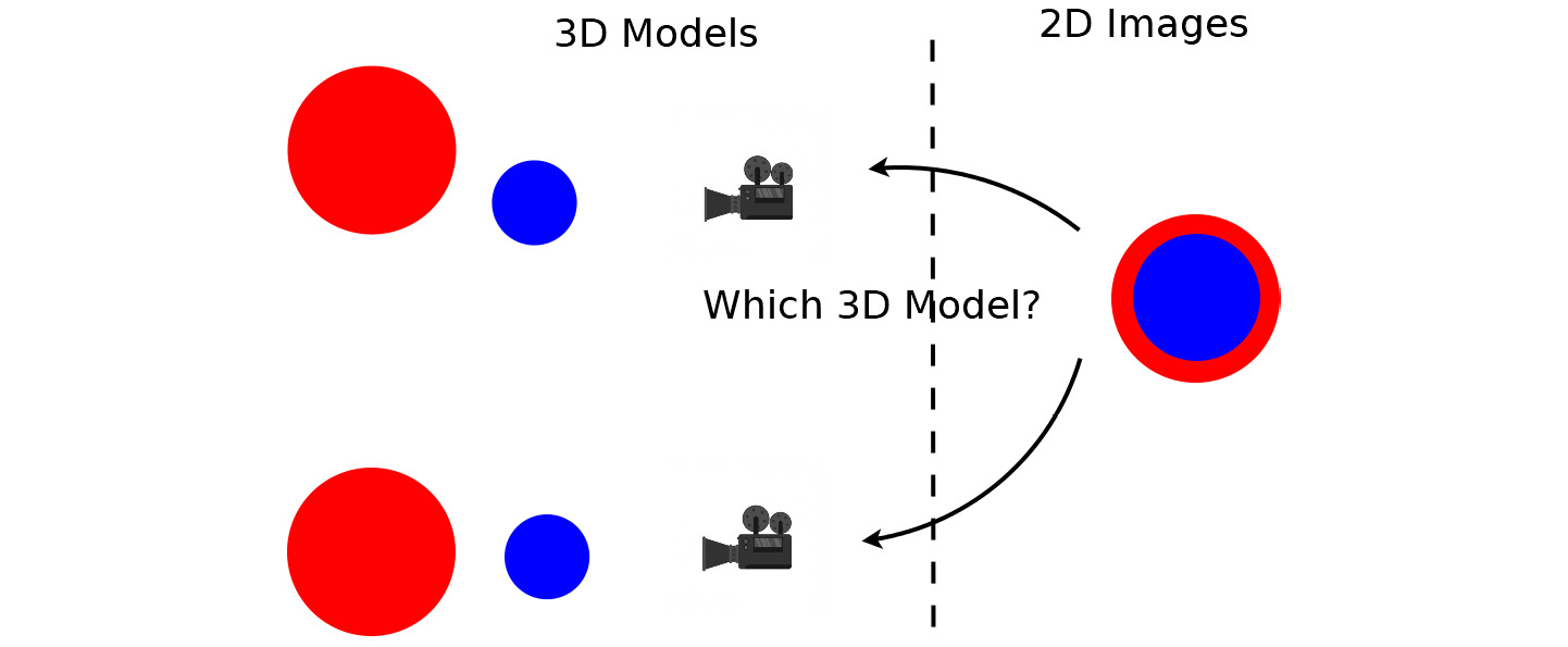
Figure 4.2: Many 3D computer vision problems are based on 2D images given to estimate 3D models
According to some ideas that were first discussed in the computer vision community decades ago, we can formulate the problem as an optimization problem. In this case, the optimization variables here are the position of two 3D spheres. We want to optimize the two centers, such that the rendered images are like the preceding 2D observed image. To measure similarity precisely, we need to use a cost function – for example, we can use pixel-wise mean-square errors. We then need to compute a gradient from the cost function to the two centers of spheres, so that we can minimize the cost function iteratively by going toward the gradient descent direction.
However, we can calculate a gradient from the cost function to the optimization variables only under the condition that the mapping from the optimization variables to the cost functions is differentiable, which implies that the rendering process is also differentiable.
How to make rendering differentiable
In this section, we are going to discuss why the conventional rendering algorithms are not differentiable. We will discuss the approach used in PyTorch3D, which makes the rendering differentiable.
Rendering is an imitation of the physical process of image formation. This physical process of image formation itself is differentiable in many cases. Suppose that the surface is normal and the material properties of the object are all smooth. Then, the pixel color in the example is a differentiable function of the positions of the spheres.
However, there are cases where the pixel color is not a smooth function of the position. This can happen at the occlusion boundaries, for example. This is shown in Figure 4.3, where the blue sphere is at a location that would occlude the red sphere at that view if the blue sphere moved up a little bit. The pixel moved at that view is thus not a differentiable function of the sphere center locations.

Figure 4.3: The image formation is not a smooth function at occlusion boundaries
When we use conventional rendering algorithms, information about local gradients is lost due to discretization. As we discussed in the previous chapters, rasterization is a step of rendering where for each pixel on the imaging plane, we find the most relevant mesh face (or decide that no relevant mesh face can be found).
In conventional rasterization, for each pixel, we generate a ray from the camera center going through the pixel on the imaging plane. We will find all the mesh faces that intersect with this ray. In the conventional approach, the rasterizer will only return the mesh face that is nearest to the camera. The returned mesh face will then be passed to the shader, which is the next step of the rendering pipeline. The shader will then be applied to one of the shading algorithms (such as the Lambertian model or Phong model) to determine the pixel color. This step of choosing the mesh to render is a non-differentiable process, since it is mathematically modeled as a step function.
There has been a large body of literature in the computer vision community on how to make rendering differentiable. The differentiable rendering implemented in the PyTorch3D library mainly used the approach in Soft Rasterizer by Liu, Li, Chen, and Li (arXiv:1904.01786).
The main idea of differentiable rendering is illustrated in Figure 4.4. In the rasterization step, instead of returning only one relevant mesh face, we will find all the mesh faces, such that the distance of the mesh face to the ray is within a certain threshold. In PyTorch3D, this threshold can be set at RasterizationSettings.blur_radius. We can also control the maximal number of faces to be returned by setting RasterizationSettings.faces_per_pixel.
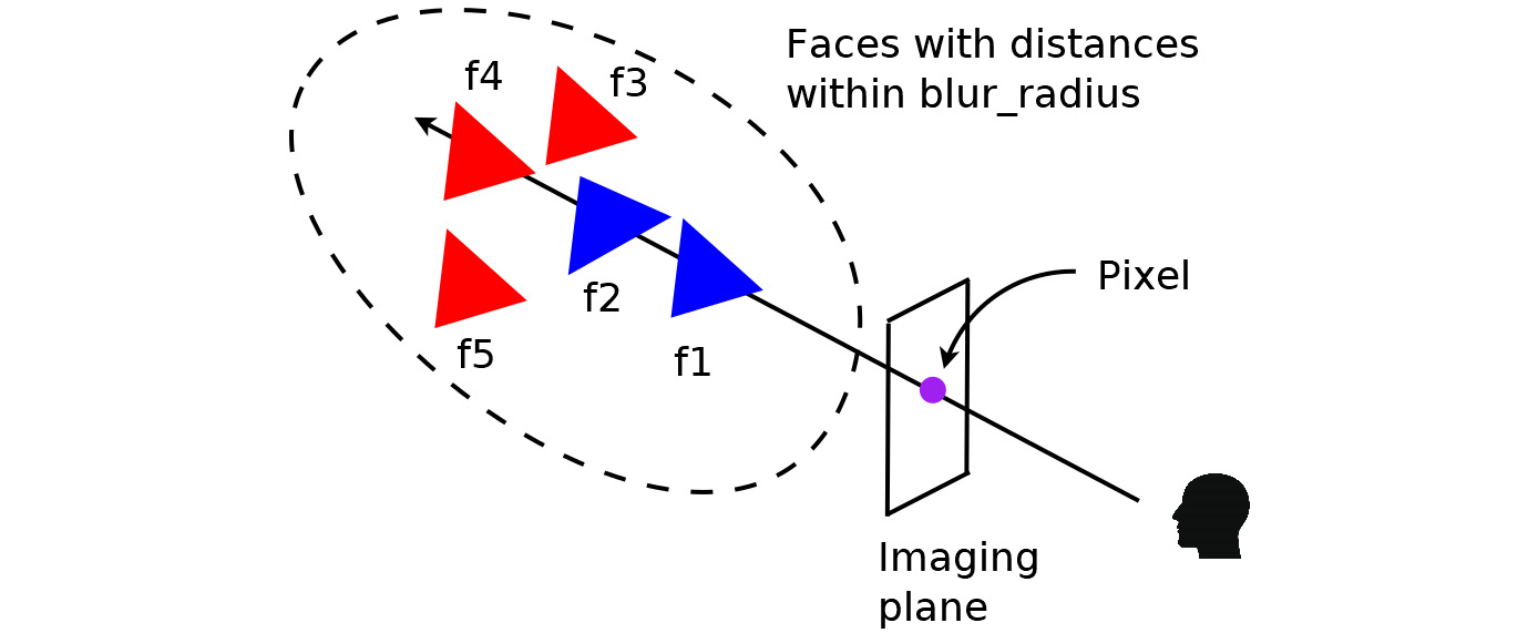
Figure 4.4: Differentiable rendering by weighted averaging of all the relevant mesh faces
Next, the renderer needs to calculate a probability map for each mesh face as follows, where dist represents the distance between the mesh face and the ray, and sigma is a hyperparameter. In Pytorch3D, the sigma parameter can be set at BlendParams.sigma. Simply put, this probability map is a probability that this mesh face covers this image pixel. The distance can be negative if the ray intersects the mesh face.

Next, the pixel color is determined by the weighted averages of the shading results of all the mesh faces returned by the rasterizer. The weight for each mesh face depends on its inverse depth value, z, and probability map, D, as shown in the following equation. Because this z value is the inverse depth, any mesh faces closer to the camera have larger z values than the mesh faces far away from the camera. The weight, wb, is a small weight for the background color. The parameter gamma here is a hyperparameter. In PyTorch3D, this parameter can be set to BlendParams.gamma:

Thus, the final pixel color can be determined by the following equation:

The PyTorch3D implementation of differential rendering also computes an alpha value for each image pixel. This alpha value represents how likely the image pixel is in the foreground, the ray intersects at least one mesh face, as shown in Figure 4.4. We want to compute this alpha value and make it differentiable. In a soft rasterizer, the alpha value is computed from the probability maps, as follows.

Now that we have learned how to make rendering differentiable, we will see how to use it for various purposes.
What problems can be solved by using differentiable rendering
As mentioned earlier, differentiable rendering has been discussed in the computer vision community for decades. In the past, differentiable rendering was used for single-view mesh reconstruction, image-based shape fitting, and more. In the following sections of this chapter, we are going to show a concrete example of using differentiable rendering for rigid object pose estimation and tracking.
Differentiable rendering is a technique in that we can formulate the estimation problems in 3D computer vision into optimization problems. It can be applied to a wide range of problems. More interestingly, one exciting recent trend is to combine differentiable rendering with deep learning. Usually, differentiable rendering is used as the generator part of the deep learning models. The whole pipeline can thus be trained end to end.
The object pose estimation problem
In this section, we are going to show a concrete example of using differentiable rendering for 3D computer vision problems. The problem is object pose estimation from one single observed image. In addition, we assume that we have the 3D mesh model of the object.
For example, we assume we have the 3D mesh model for a toy cow and teapot, as shown in Figure 4.5 and Figure 4.7 respectively. Now, suppose we have taken one image of the toy cow and teapot. Thus, we have one RGB image of the toy cow, as shown in Figure 4.6, and one silhouette image of the teapot, as shown in Figure 4.8. The problem is then to estimate the orientation and location of the toy cow and teapot at the moments when these images are taken.
Because it is cumbersome to rotate and move the meshes, we choose instead to fix the orientations and locations of the meshes and optimize the orientations and locations of the cameras. By assuming that the camera orientations are always pointing toward the meshes, we can further simplify the problem, such that all we need to optimize is the camera locations.
Thus, we formulate our optimization problem, such that the optimization variables will be the camera locations. By using differentiable rendering, we can render RGB images and silhouette images for the two meshes. The rendered images are compared with the observed images and, thus, loss functions between the rendered images and observed images can be calculated. Here, we use mean-square errors as the loss function. Because everything is differentiable, we can then compute gradients from the loss functions to the optimization variables. Gradient descent algorithms can then be used to find the best camera positions, such that the rendered images are matched to the observed images.

Figure 4.5: Mesh model for a toy cow
The following image shows the RGB output for the cow:
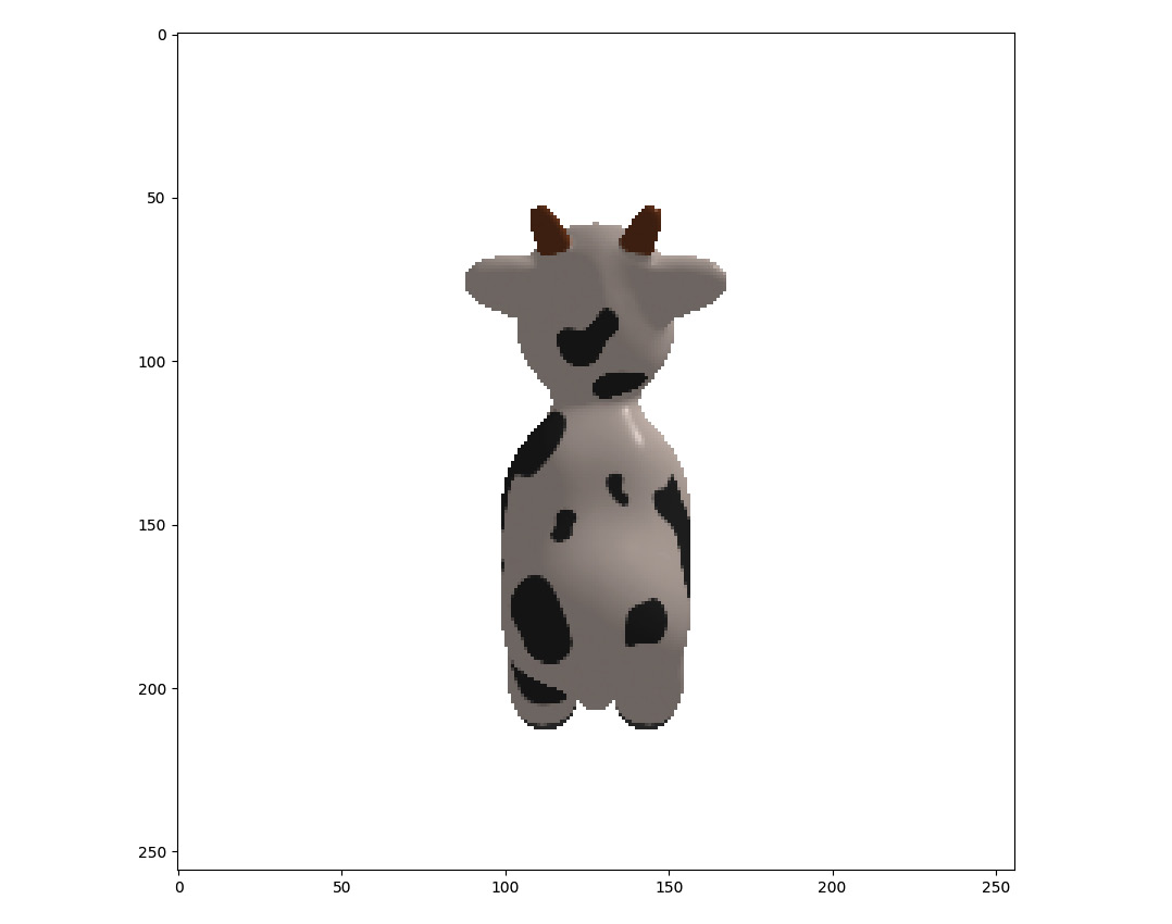
Figure 4.6: Observed RGB image for the toy cow
The following figure shows the mesh for a teapot:
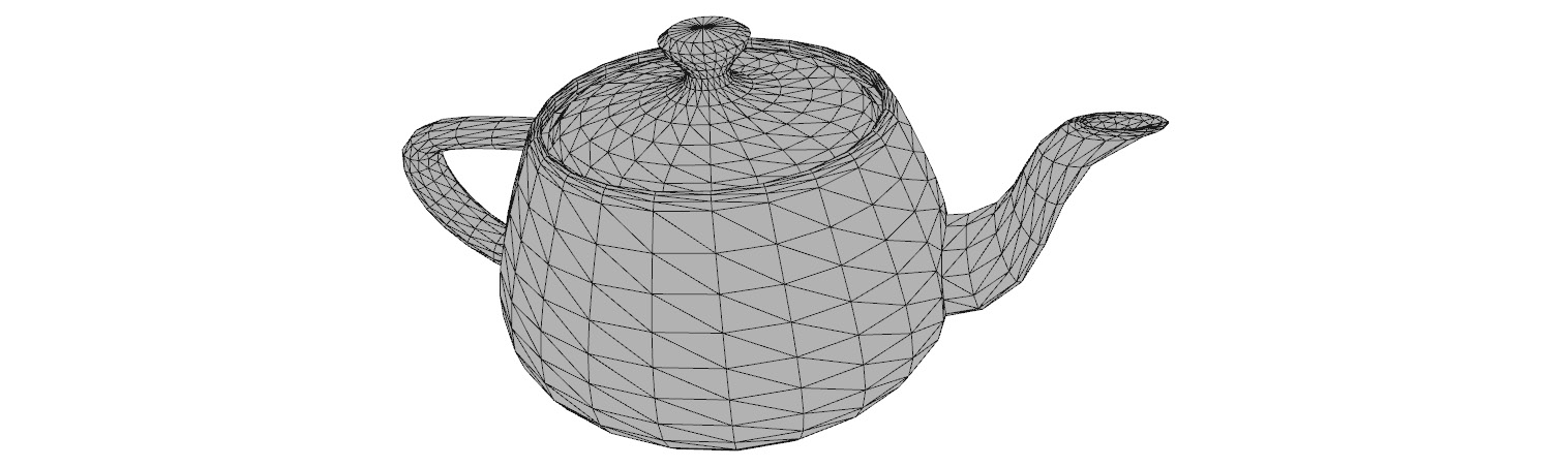
Figure 4.7: Mesh model for a teapot
The following figure shows the silhouette of the teapot:
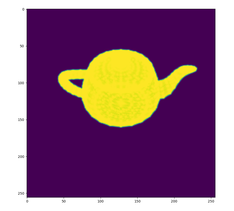
Figure 4.8: Observed silhouette of the teapot
Now that we know the problem and how to work on it, let’s start coding in the next section.
How it is coded
The code is provided in the repository in the chap4 folder as diff_render.py. The mesh model of the teapot is provided in the data subfolder as teapot.obj. We will run through the code as follows:
- The code in diff_render.py starts by importing the needed packages:
import os
import torch
import numpy as np
import torch.nn as nn
import matplotlib.pyplot as plt
from skimage import img_as_ubyte
from pytorch3d.io import load_obj
from pytorch3d.structures import Meshes
from pytorch3d.renderer import (
FoVPerspectiveCameras, look_at_view_transform, look_at_rotation,
RasterizationSettings, MeshRenderer, MeshRasterizer, BlendParams,
SoftSilhouetteShader, HardPhongShader, PointLights, TexturesVertex,
)
- In the next step, we declare a PyTorch device. If you have GPUs, then the device will be created to use GPUs. Otherwise, the device has to use CPUs:
if torch.cuda.is_available():
device = torch.device("cuda:0")
else:
device = torch.device("cpu")
print("WARNING: CPU only, this will be slow!")
- We then define output_dir in the following line. When we run the codes in diff_render.py, the codes will generate some rendered images for each optimization iteration, so that we can see how the optimization works step by step. All the generated rendered images by the code will be put in this output_dir folder.
output_dir = './result_teapot'
- We then load the mesh model from the ./data/teapot.obj file. Because this mesh model does not come with textures (material colors), we create an all-one tensor and make the tensor the texture for the mesh model. Eventually, we obtain a mesh model with textures as the teapot_mesh variable:
verts, faces_idx, _ = load_obj("./data/teapot.obj")
faces = faces_idx.verts_idx
verts_rgb = torch.ones_like(verts)[None] # (1, V, 3)
textures = TexturesVertex(verts_features=verts_rgb.to(device))
teapot_mesh = Meshes(
verts=[verts.to(device)],
faces=[faces.to(device)],
textures=textures
)
- Next, we define a camera model in the following line.
cameras = FoVPerspectiveCameras(device=device)
- In the next step, we are going to define a differentiable renderer called silhouette_renderer. Each renderer has mainly two components, such as one rasterizer for finding relevant mesh faces for each image pixel, one shader for determining the image pixel colors, and so on. In this example, we actually use a soft silhouette shader, which outputs an alpha value for each image pixel. The alpha value is a real number ranging from 0 to 1, which indicates whether this image pixel is a part of the foreground or background. Note that the hyperparameters for the shader are defined in the blend_params variables, the sigma parameter is for computing the probability maps, and gamma is for computing weights for mesh faces.
Here, we use MeshRasterizer for rasterization. Note that the parameter blur_radius is the threshold for finding relevant mesh faces and faces_per_pixel is the maximum number of mesh faces that will be returned for each image pixel:
blend_params = BlendParams(sigma=1e-4, gamma=1e-4)
raster_settings = RasterizationSettings(
image_size=256,
blur_radius=np.log(1. / 1e-4 - 1.) * blend_params.sigma,
faces_per_pixel=100,
)
silhouette_renderer = MeshRenderer(
rasterizer=MeshRasterizer(
cameras=cameras,
raster_settings=raster_settings
),
shader=SoftSilhouetteShader(blend_params=blend_params)
)
- We then define phong_renderer as follows. This phong_renderer is mainly used for visualization of the optimization process. Basically, at each optimization iteration, we will render one RGB image according to the camera position at that iteration. Note that this renderer is only used for visualization purposes, thus it is not a differentiable renderer. You can actually tell that phong_renderer is not a differentiable one by noticing the following:
- It uses HardPhoneShader, which takes only one mesh face as input for each image pixel
- It uses MeshRenderer with a blur_radius value of 0.0 and faces_per_pixel is set to 1
- A light source, lights, is then defined with a location of 2.0, 2.0, and -2.0:
raster_settings = RasterizationSettings(
image_size=256,
blur_radius=0.0,
faces_per_pixel=1,
)
lights = PointLights(device=device, location=((2.0, 2.0, -2.0),))
phong_renderer = MeshRenderer(
rasterizer=MeshRasterizer(
cameras=cameras,
raster_settings=raster_settings
),
shader=HardPhongShader(device=device, cameras=cameras, lights=lights)
)
- Next, we define a camera location and compute the corresponding rotation, R, and displacement, T, of the camera. This rotation and displacement are the target camera position – that is, we are going to generate an image from this camera position and use the image as the observed image in our problem:
distance = 3
elevation = 50.0
azimuth = 0.0
R, T = look_at_view_transform(distance, elevation, azimuth, device=device)
- Now, we generate an image, image_ref, from this camera position. The image_ref function has four channels, RGBA – R for red, G for green, B for blue, and A for alpha values. The image_ref function is also saved as target_rgb.png for our latter inspection:
silhouette = silhouette_renderer(meshes_world=teapot_mesh, R=R, T=T)
image_ref = phong_renderer(meshes_world=teapot_mesh, R=R, T=T)
silhouette = silhouette.cpu().numpy()
image_ref = image_ref.cpu().numpy()
plt.figure(figsize=(10, 10))
plt.imshow(silhouette.squeeze()[..., 3]) # only plot the alpha channel of the RGBA image
plt.grid(False)
plt.savefig(os.path.join(output_dir, 'target_silhouette.png'))
plt.close()
plt.figure(figsize=(10, 10))
plt.imshow(image_ref.squeeze())
plt.grid(False)
plt.savefig(os.path.join(output_dir, 'target_rgb.png'))
plt.close()
- In the next step, we are going to define a Model class. This Model class is derived from torch.nn.Module; thus, as with many other PyTorch models, automatic gradient computations can be enabled for Model.
Model has an initialization function, __init__, which takes the meshes input for mesh models, renderer for the renderer, and image_ref as the target image that the instance of Model will try to fit. The __init__ function creates an image_ref buffer by using the torch.nn.Module.register_buffer function. Just a reminder for those who are not so familiar with this part of PyTorch – a buffer is something that can be saved as a part of state_dict and moved to different devices in cuda() and cpu(), with the rest of the model’s parameters. However, the buffer is not updated by the optimizer.
The __init__ function also creates a model parameter, camera_position. As a model parameter, the camera_position variable can be updated by the optimizer. Note that the optimization variables now become the model parameters.
The Model class also has a forward member function, which can do the forward computation and backward gradient propagation. The forward function renders a silhouette image from the current camera position and computes a loss function between the rendered image with image_refer – the observed image:
class Model(nn.Module):
def __init__(self, meshes, renderer, image_ref):
super().__init__()
self.meshes = meshes
self.device = meshes.device
self.renderer = renderer
image_ref = torch.from_numpy((image_ref[..., :3].max(-1) != 1).astype(np.float32))
self.register_buffer('image_ref', image_ref)
self.camera_position = nn.Parameter(
torch.from_numpy(np.array([3.0, 6.9, +2.5], dtype=np.float32)).to(meshes.device))
def forward(self):
R = look_at_rotation(self.camera_position[None, :], device=self.device) # (1, 3, 3)
T = -torch.bmm(R.transpose(1, 2), self.camera_position[None, :, None])[:, :, 0] # (1, 3)
image = self.renderer(meshes_world=self.meshes.clone(), R=R, T=T)
loss = torch.sum((image[..., 3] - self.image_ref) ** 2)
return loss, image
- Now, we have already defined the Model class. We can then create an instance of the class and define an optimizer. Before running any optimization, we want to render an image to show the starting camera position. This silhouette image for the starting camera position will be saved to starting_silhouette.png:
model = Model(meshes=teapot_mesh, renderer=silhouette_renderer, image_ref=image_ref).to(device)
optimizer = torch.optim.Adam(model.parameters(), lr=0.05)
_, image_init = model()
plt.figure(figsize=(10, 10))
plt.imshow(image_init.detach().squeeze().cpu().numpy()[..., 3])
plt.grid(False)
plt.title("Starting Silhouette")
plt.savefig(os.path.join(output_dir, 'starting_silhouette.png'))
plt.close()
- Finally, we can run optimization iterations. During each optimization iteration, we will save the rendered image from the camera position to a file under the output_dir folder:
for i in range(0, 200):
if i%10 == 0:
print('i = ', i)
optimizer.zero_grad()
loss, _ = model()
loss.backward()
optimizer.step()
if loss.item() < 500:
break
R = look_at_rotation(model.camera_position[None, :], device=model.device)
T = -torch.bmm(R.transpose(1, 2), model.camera_position[None, :, None])[:, :, 0] # (1, 3)
image = phong_renderer(meshes_world=model.meshes.clone(), R=R, T=T)
image = image[0, ..., :3].detach().squeeze().cpu().numpy()
image = img_as_ubyte(image)
plt.figure()
plt.imshow(image[..., :3])
plt.title("iter: %d, loss: %0.2f" % (i, loss.data))
plt.axis("off")
plt.savefig(os.path.join(output_dir, 'fitting_' + str(i) + '.png'))
plt.close()
Figure 4.9 shows the observed silhouette of the object (in this case, a teapot):
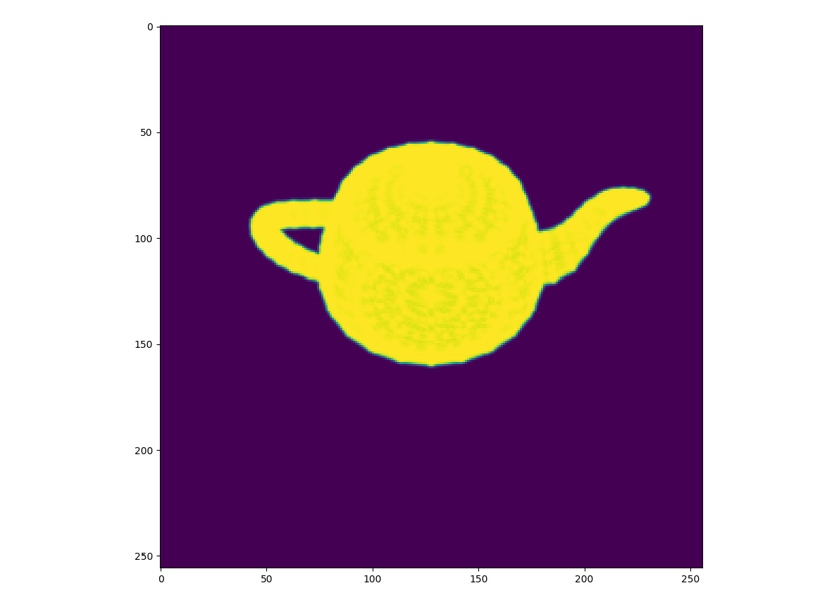
Figure 4.9: The silhouette of the teapot
We formulate the fitting problem as an optimization problem. The initial teapot position is illustrated in Figure 4.10.

Figure 4.10: The initial position of the teapot
The final optimized teapot position is illustrated in Figure 4.11.
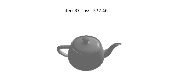
Figure 4.11: The final position of the teapot
An example of object pose estimation for both silhouette fitting and texture fitting
In the previous example, we estimated the object pose by silhouette fitting. In this section, we will present another example of object pose estimation by using both silhouette fitting and texture fitting. In 3D computer vision, we usually use texture to denote colors. Thus, in this example, we will use differentiable rendering to render RGB images according to the camera positions and optimize the camera position. The code is in diff_render_texture.py:
- In this first step, we will import all the required packages:
import os
import torch
import numpy as np
import torch.nn as nn
import matplotlib.pyplot as plt
from skimage import img_as_ubyte
from pytorch3d.io import load_objs_as_meshes
from pytorch3d.renderer import (
FoVPerspectiveCameras, look_at_view_transform, look_at_rotation,
RasterizationSettings, MeshRenderer, MeshRasterizer, BlendParams,
SoftSilhouetteShader, HardPhongShader, PointLights,
SoftPhongShader
)
- Next, we create the PyTorch device using either GPUs or CPUs:
if torch.cuda.is_available():
device = torch.device("cuda:0")
torch.cuda.set_device(device)
else:
device = torch.device("cpu")
- We set output_dir as result_cow. This will be the folder where we save the fitting results:
output_dir = './result_cow'
- We load the mesh model of a toy cow from the cow.obj file:
obj_filename = "./data/cow_mesh/cow.obj"
cow_mesh = load_objs_as_meshes([obj_filename], device=device)
- We define cameras and light sources as follows:
cameras = FoVPerspectiveCameras(device=device)
lights = PointLights(device=device, location=((2.0, 2.0, -2.0),))
- Next, we create a renderer_silhouette renderer. This is the differentiable renderer for rendering silhouette images. Note the blur_radius and faces_per_pixel numbers. This renderer is mainly used in silhouette fitting:
blend_params = BlendParams(sigma=1e-4, gamma=1e-4)
raster_settings = RasterizationSettings(
image_size=256,
blur_radius=np.log(1. / 1e-4 - 1.) * blend_params.sigma,
faces_per_pixel=100,
)
renderer_silhouette = MeshRenderer(
rasterizer=MeshRasterizer(
cameras=cameras,
raster_settings=raster_settings
),
shader=SoftSilhouetteShader(blend_params=blend_params)
)
- Next, we create a renderer_textured renderer. This renderer is another differentiable renderer, mainly used for rendering RGB images:
sigma = 1e-4
raster_settings_soft = RasterizationSettings(
image_size=256,
blur_radius=np.log(1. / 1e-4 - 1.)*sigma,
faces_per_pixel=50,
)
renderer_textured = MeshRenderer(
rasterizer=MeshRasterizer(
cameras=cameras,
raster_settings=raster_settings_soft
),
shader=SoftPhongShader(device=device,
cameras=cameras,
lights=lights)
)
- Next, we create a phong_renderer renderer. This renderer is mainly used for visualization. The preceding differentiable renders tend to create blurry images. Therefore, it would be nice for us to have a renderer that can create sharp images:
raster_settings = RasterizationSettings(
image_size=256,
blur_radius=0.0,
faces_per_pixel=1,
)
phong_renderer = MeshRenderer(
rasterizer=MeshRasterizer(
cameras=cameras,
raster_settings=raster_settings
),
shader=HardPhongShader(device=device, cameras=cameras, lights=lights)
)
- Next, we will define a camera position and the corresponding camera rotation and position. This will be the camera position where the observed image is taken. As in the previous example, we optimize the camera orientation and position instead of the object orientation and position. Also, we assume that the camera is always pointing toward the object. Thus, we only need to optimize the camera position:
distance = 3
elevation = 50.0
azimuth = 0.0
R, T = look_at_view_transform(distance, elevation, azimuth, device=device)
- Next, we create the observed images and save them to target_silhouette.png and target_rgb.png. The images are also stored in the silhouette and image_ref variables:
silhouette = renderer_silhouette(meshes_world=cow_mesh, R=R, T=T)
image_ref = phong_renderer(meshes_world=cow_mesh, R=R, T=T)
silhouette = silhouette.cpu().numpy()
image_ref = image_ref.cpu().numpy()
plt.figure(figsize=(10, 10))
plt.imshow(silhouette.squeeze()[..., 3])
plt.grid(False)
plt.savefig(os.path.join(output_dir, 'target_silhouette.png'))
plt.close()
plt.figure(figsize=(10, 10))
plt.imshow(image_ref.squeeze())
plt.grid(False)
plt.savefig(os.path.join(output_dir, 'target_rgb.png'))
plt.close()
- We modify the definition for the Model class as follows. The most notable changes from the previous example are that now we will render both the alpha channel image and the RGB images and compare them with the observed images. The mean-square losses at the alpha channel and RGB channels are weighted to give the final loss value:
class Model(nn.Module):
def __init__(self, meshes, renderer_silhouette, renderer_textured, image_ref, weight_silhouette, weight_texture):
super().__init__()
self.meshes = meshes
self.device = meshes.device
self.renderer_silhouette = renderer_silhouette
self.renderer_textured = renderer_textured
self.weight_silhouette = weight_silhouette
self.weight_texture = weight_texture
image_ref_silhouette = torch.from_numpy((image_ref[..., :3].max(-1) != 1).astype(np.float32))
self.register_buffer('image_ref_silhouette', image_ref_silhouette)
image_ref_textured = torch.from_numpy((image_ref[..., :3]).astype(np.float32))
self.register_buffer('image_ref_textured', image_ref_textured)
self.camera_position = nn.Parameter(
torch.from_numpy(np.array([3.0, 6.9, +2.5], dtype=np.float32)).to(meshes.device))
def forward(self):
# Render the image using the updated camera position. Based on the new position of the
# camera we calculate the rotation and translation matrices
R = look_at_rotation(self.camera_position[None, :], device=self.device) # (1, 3, 3)
T = -torch.bmm(R.transpose(1, 2), self.camera_position[None, :, None])[:, :, 0] # (1, 3)
image_silhouette = self.renderer_silhouette(meshes_world=self.meshes.clone(), R=R, T=T)
image_textured = self.renderer_textured(meshes_world=self.meshes.clone(), R=R, T=T)
loss_silhouette = torch.sum((image_silhouette[..., 3] - self.image_ref_silhouette) ** 2)
loss_texture = torch.sum((image_textured[..., :3] - self.image_ref_textured) ** 2)
loss = self.weight_silhouette * loss_silhouette + self.weight_texture * loss_texture
return loss, image_silhouette, image_textured
- Next, we create an instance of the Model class and create an optimizer:
model = Model(meshes=cow_mesh, renderer_silhouette=renderer_silhouette, renderer_textured = renderer_textured,
image_ref=image_ref, weight_silhouette=1.0, weight_texture=0.1).to(device)
optimizer = torch.optim.Adam(model.parameters(), lr=0.05)
- Finally, we run 200 optimization iterations. The rendered images are saved at each iteration:
for i in range(0, 200):
if i%10 == 0:
print('i = ', i)
optimizer.zero_grad()
loss, image_silhouette, image_textured = model()
loss.backward()
optimizer.step()
plt.figure()
plt.imshow(image_silhouette[..., 3].detach().squeeze().cpu().numpy())
plt.title("iter: %d, loss: %0.2f" % (i, loss.data))
plt.axis("off")
plt.savefig(os.path.join(output_dir, 'soft_silhouette_' + str(i) + '.png'))
plt.close()
plt.figure()
plt.imshow(image_textured.detach().squeeze().cpu().numpy())
plt.title("iter: %d, loss: %0.2f" % (i, loss.data))
plt.axis("off")
plt.savefig(os.path.join(output_dir, 'soft_texture_' + str(i) + '.png'))
plt.close()
R = look_at_rotation(model.camera_position[None, :], device=model.device)
T = -torch.bmm(R.transpose(1, 2), model.camera_position[None, :, None])[:, :, 0] # (1, 3)
image = phong_renderer(meshes_world=model.meshes.clone(), R=R, T=T)
plt.figure()
plt.imshow(image[..., 3].detach().squeeze().cpu().numpy())
plt.title("iter: %d, loss: %0.2f" % (i, loss.data))
plt.axis("off")
plt.savefig(os.path.join(output_dir, 'hard_silhouette_' + str(i) + '.png'))
plt.close()
image = image[0, ..., :3].detach().squeeze().cpu().numpy()
image = img_as_ubyte(image)
plt.figure()
plt.imshow(image[..., :3])
plt.title("iter: %d, loss: %0.2f" % (i, loss.data))
plt.axis("off")
plt.savefig(os.path.join(output_dir, 'hard_texture_' + str(i) + '.png'))
plt.close()
if loss.item() < 800:
break
The observed silhouette image is shown in Figure 4.12:

Figure 4.12: Observed silhouette image
The RGB image is shown in Figure 4.13:

Figure 4.13: Observed RGB image
The rendered RGB images corresponding to the initial camera position and final fitted camera position are shown in Figure 4.14 and Figure 4.15 respectively.

Figure 4.14: Image corresponding to the initial camera position
The image corresponding to the final position is as follows:
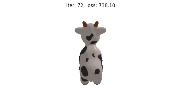
Figure 4.15: Image corresponding to the fitted camera position
Summary
In this chapter, we started with the question of why differentiable rendering is needed. The answers to this question lie in the fact that rendering can be considered as a mapping from 3D scenes (meshes or point clouds) to 2D images. If rendering is made differentiable, then we can optimize 3D models directly with a properly chosen cost function between the rendered images and observed images.
We then discussed an approach to make rendering differentiable, which is implemented in the PyTorch3D library. We then discussed two concrete examples of object pose estimation being formulated as an optimization problem, where the object pose is directly optimized to minimize the mean-square errors between the rendered images and observed images.
We also went through the code examples, where PyTorch3D is used to solve optimization problems. In the next chapter, we will explore more variations of differentiable rendering and where we can use it.