8

Modeling the Human Body in 3D

In the previous chapters, we explored ideas for modeling a 3D scene and the objects in them. Most of the objects we modeled were static and unchanging, but many applications of computer vision in real life center around humans in their natural habitat. We want to model their interactions with other humans and objects in the scene.

There are several applications for this. Snapchat filters, FaceRig, virtual try-on, and motion capture technology in Hollywood all benefit from accurate 3D body modeling. Consider, for example, an automated checkout technology. Here, a retail store is equipped with several depth-sensing cameras. They might want to detect whenever a person retrieves an object and modify their checkout basket accordingly. Such an application and many more will require us to accurately model the human body.

Human pose estimation is a cornerstone problem of human body modeling. Such a model can predict the location of joints such as shoulders, hips, and elbows to create a skeleton of the person in an image. They are then used for several downstream applications such as action recognition and human-object interaction. However, modeling a human body as a set of joints has its limitations:

• Human joints are not visible and never interact with the physical world. So, we cannot rely on them to accurately model human-object interactions.
• Joints do not model the topology, volume, and surface of the body. For certain applications, such as modeling how clothing fits, joints alone are not useful.

We can come to an agreement that human pose models are functional for some applications but certainly not realistic. How can we realistically model the human body? Will that address these limitations? What other applications can this unlock? We answer these questions in this chapter. Concretely, we will cover the following topics:

• Formulating the 3D modeling problem
• Understanding the Linear Blend Skinning technique
• Understanding the SMPL model
• Using the SMPL model
• Estimating 3D human pose and shape using SMPLify
• Exploring SMPLify

Technical requirements

The computation requirements for the code in this chapter are pretty low. However, running this in a Linux environment is recommended since it has better support for certain libraries. However, it is not impossible to run this in other environments. In the coding sections, we describe in detail how to set up the environment to successfully run the code. We will need the following technical requirements for this chapter:

• Python 2.7
• Libraries such as opendr, matplotlib, opencv, and numpy.

The code snippets for this chapter can be found at https://github.com/PacktPublishing/3D-Deep-Learning-with-Python.

Formulating the 3D modeling problem

“All models are wrong, but some are useful” is a popular aphorism in statistics. It suggests that it is often hard to mathematically model all the tiny details of a problem. A model will always be an approximation of reality, but some models are more accurate and, therefore, more useful than others.

In the field of machine learning, modeling a problem generally involves the following two components:

• Mathematically formulating the problem
• Building algorithms to solve that problem under the constraints and boundaries of that formulation

Good algorithms used on badly formulated problems often result in sub-optimal models. However, less powerful algorithms applied to a well-formulated model can sometimes result in great solutions. This insight is especially true for building 3D human body models.

The goal of this modeling problem is to create realistic animated human bodies. More importantly, this should represent realistic body shapes and must deform naturally according to changes in body pose and capture soft tissue motions. Modeling the human body in 3D is a hard challenge. The human body has a mass of bones, organs, skin, muscles, and water and they interact with each other in complex ways. To exactly model the human body, we need to model the behavior of all these individual components and their interactions with each other. This is a hard challenge, and for some practical applications, this level of exactness is unnecessary. In this chapter, we will model the human body’s surface and shape in 3D as a proxy for modeling the entire human body. We do not need the model to be exact; we just need it to have a realistic external appearance. This makes the problem more approachable.

Defining a good representation

The goal is to represent the human body accurately with a low-dimensional representation. Joint models are low-dimensional representations (typically 17 to 25 points in 3D space) but do not carry a lot of information about the shape and texture of the person. On another end, we can consider the voxel grid representation. This can model the 3D body shape and texture, but it is extremely highly dimensional and does not naturally lend itself to modeling body dynamics due to pose changes.

Therefore, we need a representation that can jointly represent body joints and surfaces, which contains information about body volume. There are several candidate representations for surfaces; one such representation is a mesh of vertices. The Skinned Multi-Person Linear (SMPL) model uses this representation. Once specified, this mesh of vertices will describe the 3D shape of a human body.

Because there is a lot of history to this problem, we will find that many artists in the character animation industry have worked on building good body meshes. The SMPL model uses such expert insights to build a good initial template of a body mesh. This is an important first step because certain parts of the body have high-frequency variations (such as the face and hands). Such high-frequency variations need more densely packed points to describe them, but body parts with lower frequency variations (such as thighs) need less dense points to accurately describe them. Such a hand-crafted initial mesh will help bring down the dimensionality of the problem while keeping the necessary information to accurately model it. This mesh in the SMPL model is gender-neutral, but you can build variations for men and women separately.

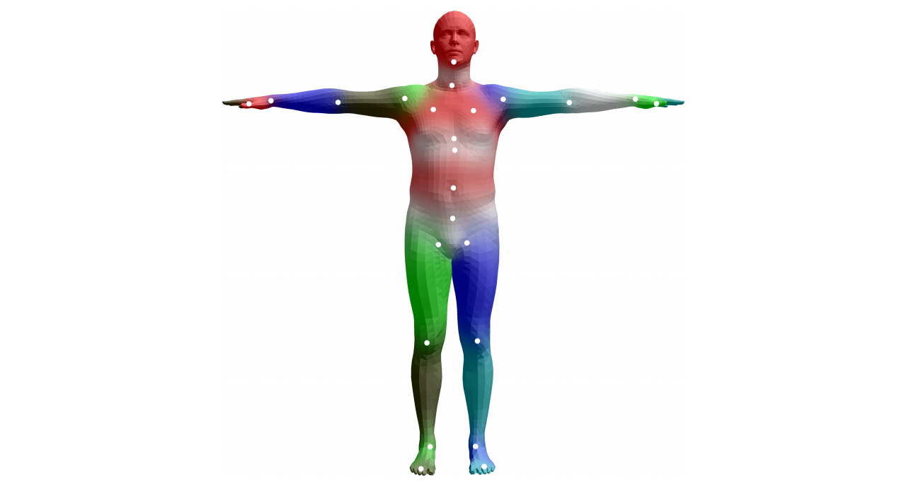
Figure 8.1 – The SMPL model template mesh in the resting pose

More concretely, the initial template mesh consists of 6,890 points in 3D space to represent the human body surface. When this is vectorized, this template mesh has a vector length of 6,890 x 3 = 20,670. Any human body can be obtained by distorting this template mesh vector to fit the body surface.

It sounds like a remarkably simple concept on paper, but the number of configurations of a 20,670-dimensional vector is extremely high. The set of configurations that represents a real human body is an extremely tiny subset of all the possibilities. The problem then becomes defining a method to obtain a plausible configuration that represents a real human body.

Before we understand how the SMPL model is designed, we need to learn about skinning models. In the next section, we will look at one of the simplest skinning techniques: the Linear Blend Skinning technique. This is important because the SMPL model is built on top of this technique.

Understanding the Linear Blend Skinning technique

Once we have a good representation of the 3D human body, we want to model how it looks in different poses. This is particularly important for character animation. The idea is that skinning involves enveloping an underlying skeleton with a skin (a surface) that conveys the appearance of the object being animated. This is a term used in the animation industry. Typically, this representation takes the form of vertices, which are then used to define connected polygons to form the surface.

The Linear Blend Skinning model is used to take a skin in the resting pose and transform it into a skin in any arbitrary pose using a simple linear model. This is so efficient to render that many game engines support this technique, and it is also used to render game characters in real time.

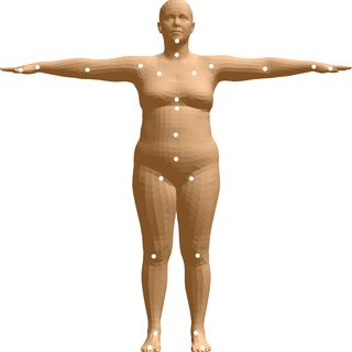
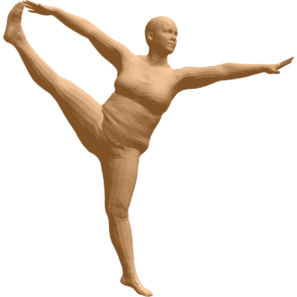
Figure 8.2 – Initial blend shape (left) and deformed mesh generated with blend skinning (right)

Let us now understand what this technique involves. This technique is a model that uses the following parameters:

• A template mesh, T, with N vertices. In this case, N = 6,890.
• We have the K joint locations represented by the vector J. These joints correspond to joints in the human body (such as shoulders, wrists, and ankles). There are 23 of these joints (K = 23).
• Blend weights, W. This is typically a matrix of size N x K that captures the relationship between the N surface vertices and the K joints of the body.
• The pose parameters, Ɵ. These are the rotation parameters for each of the K joints. There are 3K of these parameters. In this case, we have 72 of them. 69 of these parameters correspond to 23 joints and 3 correspond to the overall body rotation.

The skinning function takes the resting pose mesh, the joint locations, the blend weights, and the pose parameters as input and produces the output vertices:

In Linear Blend Skinning, the function takes the form of a simple linear function of the transformed template vertices as described in the following equation:

The meaning of these terms is the following:

• t_i represents the vertices in the original mesh in the resting pose.
• G(Ɵ, J) is the matrix that transforms the joint k from the resting pose to the target pose.
• w_k, i are elements of the blend weights, W. They represent the amount of influence the joint k has on the vertex i.

While this is an easy-to-use linear model and is very well used in the animation industry, it does not explicitly preserve volume. Therefore, transformations can look unnatural.

In order to fix this problem, artists tweak the template mesh so that when the skinning model is applied, the outcome looks natural and realistic. Such linear deformations applied to the template mesh to obtain realistic-looking transformed mesh are called blend shapes. These blend shapes are artist-designed for all of the different poses the animated character can have. This is a very time-consuming process.

As we will see later, the SMPL model automatically calculates the blend shapes before applying the skinning model to them. In the next section, you will learn about how the SMPL model creates such pose-dependent blend shapes and how data is used to guide it.

Understanding the SMPL model

As the acronym of SMPL suggests, this is a learned linear model trained on data from thousands of people. This model is built upon concepts from the Linear Blend Skinning model. It is an unsupervised and generative model that generates a 20,670-dimensional vector using the provided input parameters that we can control. This model calculates the blend shapes required to produce the correct deformations for varying input parameters. We need these input parameters to have the following important properties:

• It should correspond to a real tangible attribute of the human body.
• The features must be low-dimensional in nature. This will enable us to easily control the generative process.
• The features must be disentangled and controllable in a predictable manner. That is, varying one parameter should not change the output characteristics attributed to other parameters.

Keeping these requirements in mind, the creators of the SMPL model came up with the two most important input attributes: some notion of body identity and body pose. The SMPL model decomposes the final 3D body mesh into an identity-based shape and pose-based shape (identity-based shape is also referred to as shape-based shape because the body shape is tied to a person’s identity). This gives the model the desired property of feature disentanglement. There are some other important factors such as breathing and soft tissue dynamics (when the body is in motion) that we do not explain in this chapter but are part of the SMPL model.

Most importantly, the SMPL model is an additive model of deformations. That is, the desired output body shape vector is obtained by adding deformations to the original template body vector. This additive property makes this model very intuitive to understand and optimize.

Defining the SMPL model

The SMPL model builds on top of the standard skinning models. It makes the following changes to it:

• Rather than using the standard resting pose template, it uses a template mesh that is a function of the body shape and poses
• Joint locations are a function of the body shape

The function specified by the SMPL model takes the following form:

The following is the meaning of the terms in the preceding definitions:

• β is a vector representing the identity (also called the shape) of the body. We will later learn more about what it represents.
• Ɵ is the pose parameter corresponding to the target pose.
• W is the blend weight from the Linear Blend Skinning model.

This function looks very similar to the Linear Blend Skinning model. In this function, the template mesh is a function of shape and pose parameters, and the joint’s location is a function of shape parameters. This is not the case in the Linear Blend Skinning model.

Shape and pose-dependent template mesh

The redefined template mesh is an additive linear deformation of the standard template mesh:

Here, we see the following:

• is an additive deformation from the body shape parameters β. It is a learned deformation modeled as the first few principal components of the shape displacements. These principal components are obtained from the training data involving different people in the same resting pose.
• is an additive pose deformation term. This is parametrized by Ɵ. This is also a linear function learned from a multi-pose dataset of people in different poses.

Shape-dependent joints

Since joint locations depend on the body shape, they are redefined as a function of body shape. The SMPL model defines this in the following manner:

Here, is the additive deformation from the body shape parameters β, and J is a matrix that transforms the rest template vertices to the rest template poses. The parameters of J are also learned from data.

Using the SMPL model

Now that you have a high-level understanding of the SMPL model, we will look at how to use it to create 3D models of humans. In this section, we will start with a few basic functions; this will help you explore the SMPL model. We will load the SMPL model, and edit the shape and pose parameters to create a new 3D body. We will then save this as an object file and visualize it.

This code was originally created by the authors of SMPL for python2. Therefore, we need to create a separate python2 environment. The following are the instructions for this:

cd chap8

conda create -n python2 python=2.7 anaconda

source activate python2

pip install –r requirements.txt

This creates and activates the Python 2.7 conda environment and installs the required modules. Python 2.7 is being deprecated, so you might see warning messages when you try to use it. In order to create a 3D human body with random shape and pose parameters, run the following command.

$ python render_smpl.py

This will pop up a window that shows the rendering of a human body in 3D. Our output will likely be different since render_smpl.py creates a human body with random pose and shape parameters.

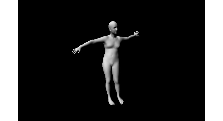
Figure 8.3 – An example rendering of the hello_smpl.obj created by explore_smpl.py

Now that we have run the code and obtained a visual output, let us explore what is happening in the render_smpl.py file:

1. Import all of the required modules:

   import cv2

   import numpy as np

   from opendr.renderer import ColoredRenderer

   from opendr.lighting import LambertianPointLight

   from opendr.camera import ProjectPoints

   from smpl.serialization import load_model

2. Load the model weights of the basic SMPL model. Here, we load the neural body model:

   m = load_model('../smplify/code/models/basicModel_neutral_lbs_10_207_0_v1.0.0.pkl')

3. Next, we assign random pose and shape parameters. The following pose and shape parameters dictate how the 3D body mesh looks in the end:

   m.pose[:] = np.random.rand(m.pose.size) * .2

   m.betas[:] = np.random.rand(m.betas.size) * .03

   m.pose[0] = np.pi

4. We now create a renderer and assign attributes to it, and we construct the light source. By default, we use the OpenDR renderer, but you can switch this to use the PyTorch3D renderer and light source. Before doing that, make sure to address any Python incompatibility issues.

   rn = ColoredRenderer()

   w, h = (640, 480)

   rn.camera = ProjectPoints(v=m, rt=np.zeros(3), t=np.array([0, 0, 2.]), f=np.array([w,w])/2., c=np.array([w,h])/2., k=np.zeros(5))

   rn.frustum = {'near': 1., 'far': 10., 'width': w, 'height': h}

   rn.set(v=m, f=m.f, bgcolor=np.zeros(3))

   rn.vc = LambertianPointLight(f=m.f, v=rn.v, num_verts=len(m), light_pos=np.array([-1000,-1000,-2000]), vc=np.ones_like(m)*.9, light_color=np.array([1., 1., 1.]))

5. We can now render the mesh and display it in an OpenCV window:

   cv2.imshow('render_SMPL', rn.r)

   cv2.waitKey(0)

   cv2.destroyAllWindows()

We have now used the SMPL model to generate a random 3D human body. In reality, we might be interested in generating 3D shapes that are more controllable. We will look at how to do this in the next section.

Estimating 3D human pose and shape using SMPLify

In the previous section, you explored the SMPL model and used it to generate a 3D human body with a random shape and pose. It is natural to wonder whether it is possible to use the SMPL model to fit a 3D human body onto a person in a 2D image. This has multiple practical applications, such as understanding human actions or creating animations from 2D videos. This is indeed possible, and in this chapter, we are going to explore this idea in more detail.

Imagine that you are given a single RGB image of a person without any information about body pose, camera parameters, or shape parameters. Our goal is to deduce the 3D shape and pose from just this single image. Estimating the 3D shape from a 2D image is not always error-free. It is a challenging problem because of the complexity of the human body, articulation, occlusion, clothing, lighting, and the inherent ambiguity in inferring 3D from 2D (because multiple 3D poses can have the same 2D pose when projected). We also need an automatic way of estimating this without much manual intervention. It also needs to work on complex poses in natural images with a variety of backgrounds, lighting conditions, and camera parameters.

One of the best methods of doing this was invented by researchers from the Max Planck Institute of Intelligent Systems (where the SMPL model was invented), Microsoft, the University of Maryland, and the University of Tübingen. This approach is called SMPLify. Let us explore this approach in more detail.

The SMPLify approach consists of the following two stages:

1. Automatically detect 2D joints using established pose detection models such as OpenPose or DeepCut. Any 2D joint detectors can be used in their place as long as they are predicting the same joints.
2. Use the SMPL model to generate the 3D shape. Directly optimize the parameters of the SMPL model so that the model joints of the SMPL model project to the 2D joints predicted in the previous stage.

We know that SMPL captures shapes from just the joints. With the SMPL model, we can therefore capture information about body shape just from the joints. In the SMPL model, the body shape parameters are characterized by β. They are the coefficients of the principal components in the PCA shape model. The pose is parametrized by the relative rotation and theta of the 23 joints in the kinematic tree. We need to fit these parameters, β and theta, so that we minimize an objective function.

Defining the optimization objective function

Any objective function must capture our intention to minimize some notion of error. The more accurate this error calculation is, the more accurate the output of the optimization step will be. We will first look at the entire objective function, then look at each of the individual components of that function and explain why each of them is necessary:

• We want to minimize this objective function by optimizing parameters β and Ɵ. It consists of four terms and corresponding coefficients, λƟ, λa, λsp, and λβ, which are hyperparameters of the optimization process. The following is what each of the individual terms means:
  • is the joint-based term that penalizes the distance between the 2D projected joint of the SMPL model and the predicted joint location from the 2D joint detector (such as DeepCut or OpenPose). w_i is the confidence score of each of the joints provided by the 2D joint detection model. When a joint is occluded, the confidence score for that joint will be low. Naturally, we should not place a lot of importance on such occluded joints.
  • is the pose that penalizes large angles between joints. For example, it ensures that elbows and knees do not bend unnaturally.
  • is a Gaussian mixture model fit on natural poses obtained from a very large dataset. This dataset is called the CMU Graphics Lab Motion Capture Database, consisting of nearly one million data points. This data-driven term in the optimization function ensures that the pose parameters are close to what we observe in reality.

1. is the self-penetration error. When the authors optimized the objective function without this error term, they saw unnatural self-penetrations, such as elbows and hands twisted and penetrating through the stomach. This is physically impossible. However, after adding this error term, they found naturally qualitative results. This error term consists of body parts that are approximated as a set of spheres. They define incompatible spheres and penalize the intersection of these incompatible spheres.
2. is the shape obtained from the SMPL model. Note here that the principal component matrix is part of the SMPL model, which was obtained by training on the SMPL training dataset.

In summary, the objective function consists of five components that, together, ensure that the solution to this objective function is a set of pose and shape parameters (theta and beta) that ensure that the 2D join projection distances are minimized while simultaneously ensuring that there are no large joint angles, no unnatural self-penetrations, and that the pose and shape parameters adhere to a prior distribution we see in a large dataset consisting of natural body poses and shapes.

Exploring SMPLify

Now that we have a broad overview of how to estimate the 3D body shape of a person in a 2D RGB image, let us get a hands-on experience with code. Concretely, we are going to fit a 3D body shape onto two 2D images from the Leeds Sports Pose (LSP) dataset. This dataset contains 2,000 pose-annotated images of mostly sportspeople gathered from Flickr. We will first run through the code and generate these fitted body shapes before we dig deeper into the code. All the code used in this section was adapted from the implementation of the paper titled Keep it SMPL: Automatic Estimation of 3D Human Pose and Shape from a Single Image. We have only adapted it in a way that helps you, the learner, to quickly run the code and visualize the outputs yourself.

This code was originally created by the authors of SMPLify for python2. Therefore, we need to use the same python2 environment we used while exploring the SMPL model. Before we run any code, let us quickly get an overview of how the code is structured:

chap8

  -- smplify

    -- code

      -- fit3d_utils.py

      -- run_fit3d.py

      -- render_model.py

      -- lib

      -- models

    -- images

    -- results

Running the code

The main file you will be directly interacting with is run_fir3d.py. The folder named images will have some example images from the LSP dataset. However, before we run the code, make sure that PYTHONPATH is set correctly. This should point to the location of the chap8 folder. You can run the following code for it:

export PYTHONPATH=$PYTHONPATH:<user-specific-path>/3D-Deep-Learning-with-Python/chap8/

Now, go to the right folder:

cd smplify/code

You can now run the following command to fit a 3D body onto images in the images folder:

python run_fit3d.py --base_dir ../ --out_dir .

This run will not use any interpenetration error since it will be faster to go through the optimization iterations. In the end, we will fit a body-neutral shape. You will be able to visualize the projected pose of the 3D body as it fits the person in the picture. Once the optimization is complete, you will see the following two images:

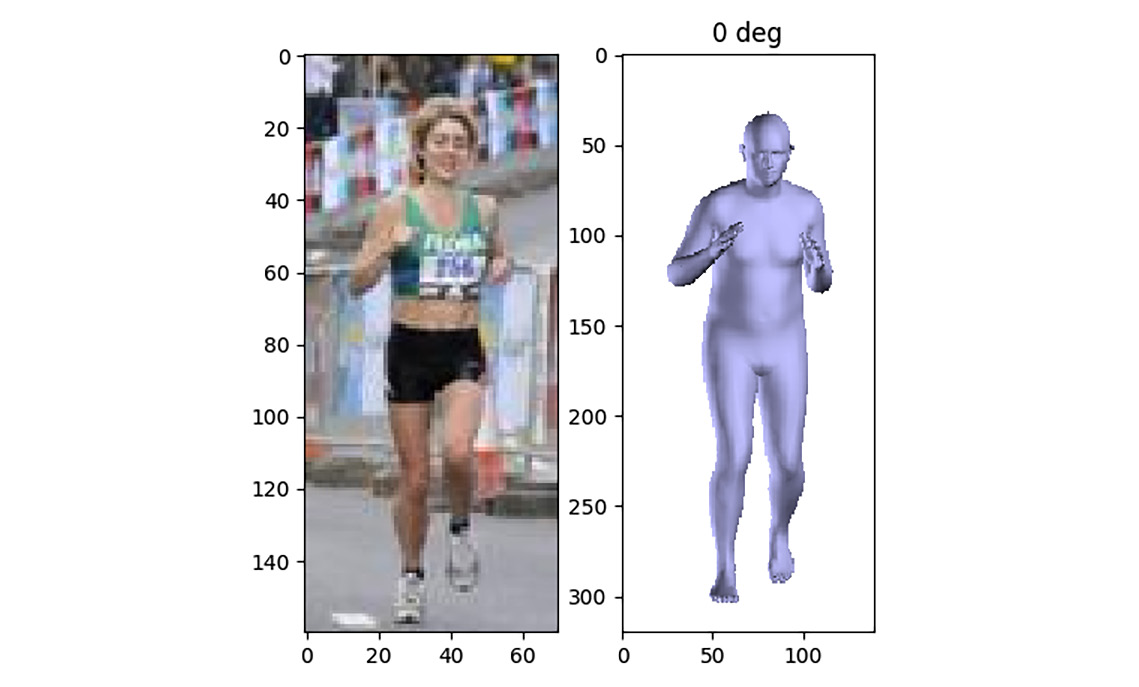
Figure 8.4 – Image in the LSP dataset of a person running (left) and the 3D body shape fitting this image (right)

Another output is as follows:

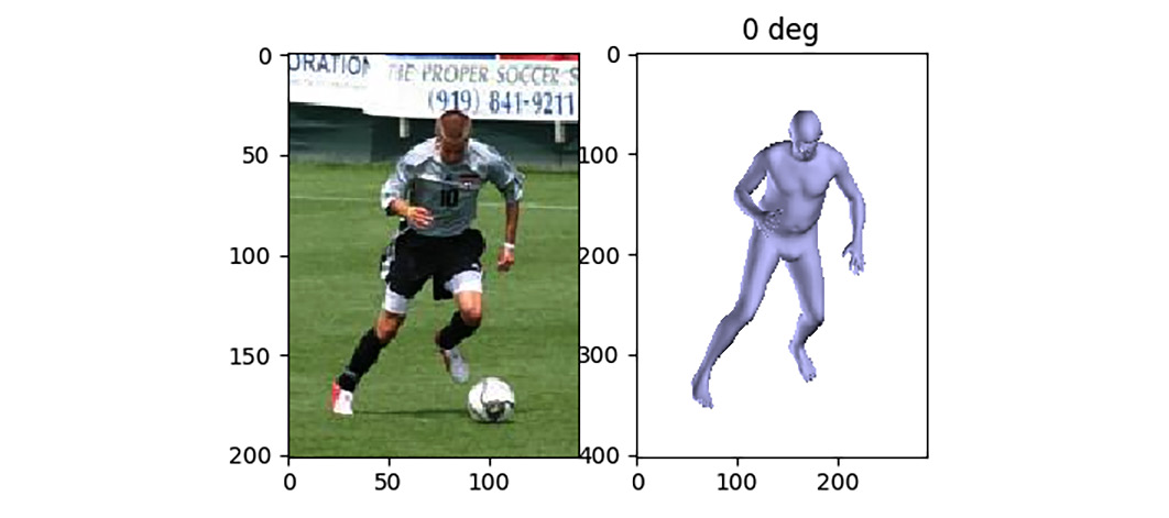
Figure 8.5 – Image in the LSP dataset of a soccer player in action (left) and the 3D body shape fitting this image (right)

Exploring the code

Now that you have run the code to fit humans in 2D images, let us look at the code in more detail to understand some of the main components needed to achieve this. You will find all the components in run_fit3d.py. You need to perform the following steps:

1. Let us first import all of the modules we will need:

   from os.path import join, exists, abspath, dirname

   from os import makedirs

   import cPickle as pickle

   from glob import glob

   import cv2

   import numpy as np

   import matplotlib.pyplot as plt

   import argparse

   from smpl.serialization import load_model

   from smplify.code.fit3d_utils import run_single_fit

2. Let us now define where our SMPL model is located. This is done through the following:

   MODEL_DIR = join(abspath(dirname(__file__)), 'models')

   MODEL_NEUTRAL_PATH = join(

   MODEL_DIR, 'basicModel_neutral_lbs_10_207_0_v1.0.0.pkl')

3. Let us set some parameters required for the optimization method and define the directories where our images and results are located. The results folder will have joint estimates for all the images in the dataset. viz is set to True to enable visualization. We are using an SMPL model with 10 parameters (that is, it uses 10 principal components to model the body shape). flength refers to the focal length of the camera; this is kept fixed during optimization. pix_thsh refers to the threshold (in pixels). If the distance between shoulder joints in 2D is lower than pix_thsh, the body orientation is ambiguous. This could happen when a person is standing perpendicular to the camera. As a consequence, it is hard to say whether they are facing left or right. So, a fit is run on both the estimated one and its flip:

   viz = True

   n_betas = 10

   flength = 5000.0

   pix_thsh = 25.0

   img_dir = join(abspath(base_dir), 'images/lsp')

   data_dir = join(abspath(base_dir), 'results/lsp')

   if not exists(out_dir):

       makedirs(out_dir)

4. We should then load this gender-neutral SMPL model into memory:

   model = load_model(MODEL_NEUTRAL_PATH)

5. We then need to load the joint estimates for the images in the LSP dataset. The LSP dataset itself contains joint estimates and corresponding joint confidence scores for all the images in the dataset. We are going to just use that directly. You can also provide your own joint estimates or use good joint estimators, such as OpenPose or DeepCut, to get the joint estimates:

   est = np.load(join(data_dir, 'est_joints.npz'))['est_joints']

6. Next, we need to load images in the dataset and get the corresponding joint estimates and confidence scores:

   img_paths = sorted(glob(join(img_dir, '*[0-9].jpg')))

   for ind, img_path in enumerate(img_paths):

       img = cv2.imread(img_path)

       joints = est[:2, :, ind].T

       conf = est[2, :, ind]

7. For each of the images in the dataset, use the run_single_fit function to fit the parameters beta and theta. The following function returns these parameters after running the optimization on an objective function similar to the SMPLify objective function we discussed in the previous section:

   params, vis = run_single_fit(img, joints, conf, model, regs=sph_regs, n_betas=n_betas, flength=flength, pix_thsh=pix_thsh, scale_factor=2, viz=viz, do_degrees=do_degrees)

While the objective function is being optimized, this function creates a matplotlib window where the green circles are the 2D joint estimates from a 2D joint detection model (which are provided to you). The red circles are the projected joints of the SMPL 3D model that is being fitted onto the 2D image:

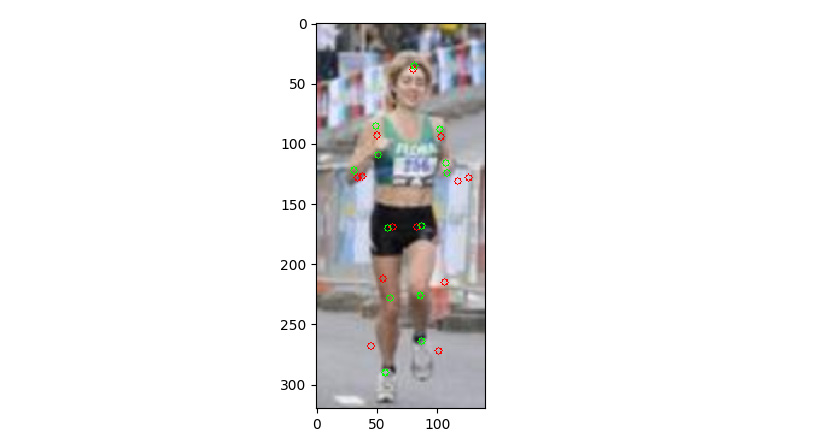
Figure 8.6 – Visualization of the provided 2D joints (green) and the projected joints (red) of the SMPL model being fit to the 2D image

8. Next, we want to visualize the fitted 3D human body alongside the 2D RGB image. We use matplotlib for this. The following opens up an interactive window where you can save images to disk:

   if viz:

       import matplotlib.pyplot as plt

       plt.ion()

       plt.show()

       plt.subplot(121)

       plt.imshow(img[:, :, ::-1])

       for di, deg in enumerate(do_degrees):

           plt.subplot(122)

           plt.cla()

           plt.imshow(vis[di])

           plt.draw()

           plt.title('%d deg' % deg)

           plt.pause(1)

           raw_input('Press any key to continue...')

9. We then want to save these parameters and visualization to disk with the following code:

       with open(out_path, 'w') as outf:

           pickle.dump(params, outf)

       if do_degrees is not None:

           cv2.imwrite(out_path.replace('.pkl', '.png'), vis[0])

In the preceding code, the most important function is run_single_fit. You can explore this function in more detail in smplify.code.fit3d_utils.py.

It is important to note here that the accuracy of the fitted 3D body is dependent on the accuracy of the 2D joints. Since the 2D joints are predicted using a joint detection model (such as OpenPose or DeepCut), the accuracy of such joint prediction models becomes very important and relevant to this problem. Estimating 2D joints is especially error-prone in the following scenarios:

• Joints that are not completely visible are hard to predict. This could happen due to a variety of reasons including self-occlusion, occlusion by other objects, unusual clothing, and so on.
• It is easy to confuse between left and right joints (for example, left wrist versus right wrist). This is especially true when the person is facing the camera sideways.
• Detecting joints in unusual poses is hard if the model is not trained with those poses. This depends on the diversity in the dataset used to train the joint detector.

More broadly, a system consisting of multiple machine learning models interacting with each other sequentially (that is, when the output of one model becomes the input of another model) will suffer from cascading errors. Small errors in one component will result in large errors in outputs from downstream components. Such a problem is typically solved by training a system end to end. However, this strategy cannot be used here at the moment since there is no ground-truth data in the research community that directly maps a 2D input image to a 3D model.

Summary

In this chapter, we got an overview of the mathematical formulation of modeling human bodies in 3D. We understood the power of good representation and used simple methods such as Linear Blend Skinning on a powerful representation to obtain realistic outputs. We then got a high-level overview of the SMPL model and used it to create a random 3D human body. Afterward, we went over the code used to generate it. Next, we looked at how SMPLify can be used to fit a 3D human body shape onto a person in a 2D RGB image. We learned about how this uses the SMPL model in the background. Moreover, we fit human body shapes to two images in the LSP dataset and understood the code we used to do this. With this, we got a high-level overview of modeling the human body in 3D.

In the next chapter, we will explore the SynSin model, which is typically used for 3D reconstruction. The goal of the next chapter is to understand how to reconstruct an image from a different view, given just a single image.