9

Performing End-to-End View Synthesis with SynSin

This chapter is dedicated to the latest state-of-the-art view synthesis model called SynSin. View synthesis is one of the main directions in 3D deep learning, which can be used in multiple different domains such as AR, VR, gaming, and more. The goal is to create a model for the given image as an input to reconstruct a new image from another view.

In this chapter, first, we will explore view synthesis and the existing approaches to solving this problem. We will discuss all advantages and disadvantages of these techniques.

Second, we are going to dive deeper into the architecture of the SynSin model. This is an end-to-end model that consists of three main modules. We will discuss each of them and understand how these modules help to solve view synthesis without any 3D data.

After understanding the whole structure of the model, we will move on to hands-on practice, where we will set up and work with the model to better understand the whole view synthesis process. We will train and test the model, and also use pre-trained models for inference.

In this chapter, we’re going to cover the following main topics:

• Overview of view synthesis
• SynSin network architecture
• Hands-on model training and testing

Technical requirements

To run the example code snippets in this book, ideally, readers need to have a computer with a GPU. However, running the code snippets with only CPUs is not impossible.

The recommended computer configuration includes the following:

• A GPU, for example, the Nvidia GTX series or the RTX series with at least 8 GB of memory
• Python 3
• The PyTorch and PyTorch3D libraries

The code snippets for this chapter can be found at https:github.com/PacktPublishing/3D-Deep-Learning-with-Python.

Overview of view synthesis

One of the most popular research directions in 3D computer vision is view synthesis. Given the data and the viewpoint, the idea of this research direction is to generate a new image that renders the object from another viewpoint.

View synthesis comes with two challenges. The model should understand the 3D structure and semantic information of the image. By 3D structure, we mean that when changing the viewpoint, we get closer to some objects and far away from others. A good model should handle this by rendering images where some objects are bigger and some are smaller to view - change. By semantic information, we mean that the model should differentiate the objects and should understand what objects are presented in the image. This is important because some objects can be partially included in the image; therefore, during the reconstruction, the model should understand the semantics of the object to know how to reconstruct the continuation of that object. For example, given an image of a car on one side where we only see two wheels, we know that there are two more wheels on the other side of the car. The model must contain these semantics during reconstruction:

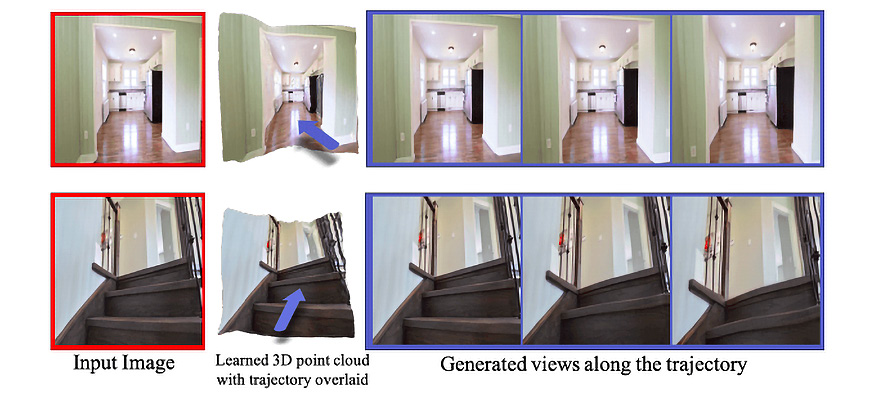
Figure 9.1: The red-framed photographs show the original image, and the blue-framed photographs show the newly generated images; this is an example of view synthesis using the SynSin methodology

Many challenges need to be addressed. For the models, it’s hard to understand the 3D scene from an image. There are several methods for view synthesis:

• View synthesis from multiple images: Deep neural networks can be used to learn the depth of multiple images, and then reconstruct new images from another view. However, as mentioned earlier, this implies that we have multiple images from slightly different views, and sometimes, it’s hard to obtain such data.
• View synthesis using ground-truth depth: This involves a group of techniques where a ground-truth mask is used beside the image, which represents the depth of the image and semantics. Although in some cases, these types of models can achieve good results, it’s hard and expensive to gather data on a large scale, especially when it comes to outdoor scenes. Also, it’s expensive and time-consuming to annotate such data on a large scale, too.
• View synthesis from a single image: This is a more realistic setting when we have only one image and we aim to reconstruct an image from the new view. It’s harder to get more accurate results by only using one image. SynSin belongs to a group of methods that can achieve a state-of-the-art view synthesis.

So, we have covered a brief overview of view synthesis. Now, we will explore SynSin, dive into the network architecture, and examine the model training and testing processes.

SynSin network architecture

The idea of SynSin is to solve the view synthesis problem with an end-to-end model using only one image at test time. This is a model that doesn’t need 3D data annotations and acheives very good accuracy compared to its baseline:

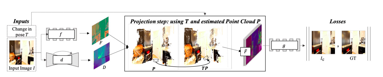
Figure 9.2: The structure of the end-to-end SynSin method

The model is trained end-to-end, and it consists of three different modules:

• Spatial feature and depth networks
• Neural point cloud renderer
• Refinement module and discriminator

Let’s dive deeper into each one to better understand the architecture.

Spatial feature and depth networks

If we zoom into the first part of Figure 9.2, we can see two different networks that are fed by the same image. These are the spatial feature network (f) and the depth network (d) (Figure 9.3):

Figure 9.3: Input and outputs of the spatial feature and depth networks

Given a reference image and the desired change in pose (T), we wish to generate an image as if that change in the pose were applied to the reference image. For the first part, we only use a reference image and feed it to two networks. A spatial feature network aims to learn feature maps, which are higher-resolution representations of the image. This part of the model is responsible for learning semantic information about the image. This model consists of eight ResNet blocks and outputs 64-dimensional feature maps for each pixel of the image. The output has the same resolution as the original image.

Next, the depth network aims to learn the 3D structure of the image. It won’t be an accurate 3D structure, as we don’t use exact 3D annotations. However, the model will further improve it. UNet with eight downsampling and upsampling layers are used for this network, followed by the sigmoid layer. Again, the output has the same resolution as the original image.

As you might have noticed, both models keep a high resolution for the output channels. This will further help to reconstruct more accurate and higher-quality images.

Neural point cloud renderer

The next step is to create a 3D point cloud that can then be used with a view transform point to render a new image from the new viewpoint. For that, we use the combined output of the spatial feature and depth networks.

The next step should be rendering the image from another point. In most scenarios, a naïve renderer would be used. This projects 3D points to one pixel or a small region in the new view. A naïve renderer uses a z-buffer, which keeps all the distances from the point to the camera. The problem with the naïve renderer is that it’s not differentiable, which means we can’t use gradients to update our depth and spatial feature networks. Moreover, we want to render features instead of RGB images. This means the naïve renderer won’t work for this technique:

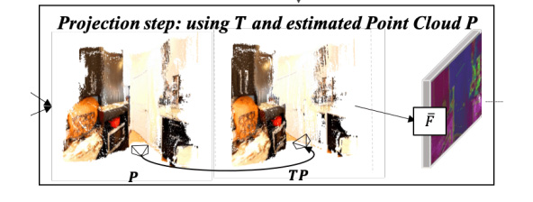
Figure 9.4: Pose transformation in the neural point cloud renderer

Why not just differentiate naïve renderers? Here, we face two problems:

• Small neighborhoods: As mentioned earlier, each point only appears on one or a few pixels of the rendered image. Therefore, there are only a few gradients for each point. This is a drawback of local gradients, which degrades the performance of the network relying on gradient updates.
• The hard z-buffer: The z-buffer only keeps the nearest point for rendering the image. If new points appear closer, suddenly the output will change drastically.

To overcome the issues presented here, the model tries to soften the hard decision. This technique is called a neural point cloud renderer. To do that, the renderer, instead of assigning a pixel for a point, splats with varying influence. This solves a small neighborhood problem. For the hard z-buffer issue, we then accumulate the effect of the nearest points, not just the nearest point:

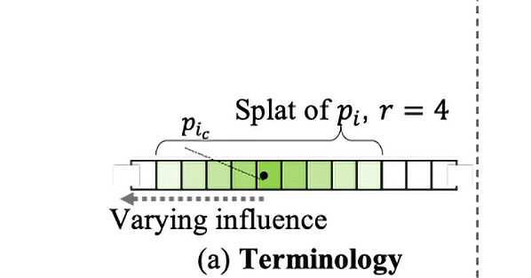
Figure 9.5: Projecting the point with the splatting technique

A 3D point is projected and splatted with radius r (Figure 9.5). Then, the influence of the 3D point on that pixel is measured by the Euclidean distance between the center of the splatted point to that point:

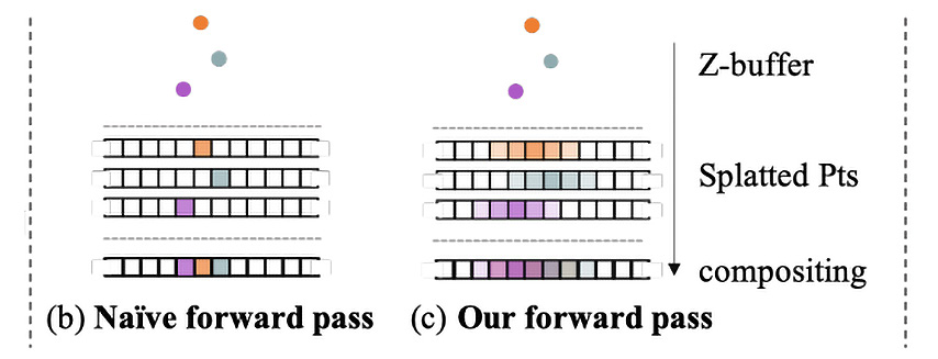
Figure 9.6: The effect of forward and backward propagation with a neural point cloud renderer on an example of naïve (b) and SynSin (c) rendering

As you can see in the preceding figure, each point is splatted, which helps us to not lose too much information and helps in solving tricky problems.

The advantage of this approach is that it allows you to gather more gradients for one 3D point, which improves the network learning process for both spatial features and depth networks:

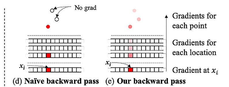
Figure 9.7: Backpropagation for the naïve renderer and the neural point cloud renderer

Lastly, we need to gather and accumulate points in the z-buffer. First, we sort points according to their distance from the new camera, and then K-nearest neighbors with alpha compositing are used to accumulate points:

Figure 9.8: 3D point cloud output

As you can see in Figure 9.8, the 3D point cloud outputs an unrefined new view. The output should then become the input of the refiner module.

Refinement module and discriminator

Last but not least, the model consists of a refinement module. This module has two missions: first to improve the accuracy of the projected feature and, second, to fill the nonvisible part of the image from the new view. It should output semantically meaningful and geometrically accurate images. For example, if only one part of the table is visible in the image and in the new view, the image should contain a larger part of it, this module should understand semantically that this is a table, and during the reconstruction, it should keep the lines of the new part geometrically correct (for instance, the straight lines should remain straight). The model learns these properties from a dataset of real-world images:

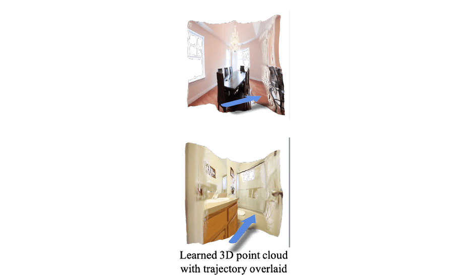
Figure 9.9: The refinement module

The refinement module (g) gets inputs from the neural point cloud renderer and then outputs the final reconstructed image. Then, it is used in loss objectives to improve the training process.

This task is solved with generative models. ResNet with eight blocks is used, and to keep the resolution of the image good, downsampling and upsampling blocks were used, too. We use GAN with two multilayer discriminators and feature matching loss on the discriminator.

The final loss of the model consists of the L1 loss, content loss, and discriminator loss between the generated and target images:

The loss function is then used for model optimization as usual.

This is how SynSin combines various modules to create an end-to-end process of synthesizing views from just one image. Next, we will explore the practical implementation of the model.

Hands-on model training and testing

Facebook Research released the GitHub repository of the SynSin model, which allows us to train the model and use an already pre-trained model for inference. In this section, we will discuss both the training process and inference with pre-trained models:

1. But first, we need to set up the model. We need to clone the GitHub repository, create an environment, and install all the requirements:

   git clone https://github.com/facebookresearch/synsin.git

   cd synsin/

   conda create –-name synsin_env –-file requirements.txt

   conda activate synsin_env

If requirements can’t be installed with the preceding command, it’s always possible to install them manually. For manual installation, follow the synsin/INSTALL.md file instructions.

2. The model was trained on three different datasets:
   1. RealEstate10K
   2. MP3D
   3. KITTI

For the training, data can be downloaded from the dataset websites. For this book, we are going to use the KITTI dataset; however, feel free to try other datasets, too.

Instructions on how to download the KITTI dataset can be found in the SynSin repository at https://github.com/facebookresearch/synsin/blob/main/KITTI.md.

First, we need to download the dataset from the website and store the files in ${KITTI_HOME}/dataset_kitti, where KITTI_HOME is the path where the dataset will be located.

3. Next, we need to update the ./options/options.py file, where we need to add the path to the KITTI dataset on our local machine:

   elif opt.dataset == 'kitti':

      opt.min_z = 1.0

      opt.max_z = 50.0

      opt.train_data_path = (

          './DATA/dataset_kitti/'

      )

      from data.kitti import KITTIDataLoader

      return KITTIDataLoader

If you are going to use another dataset, you should find the DataLoader for other datasets and add the path to that dataset.

4. Before training, we have to download pre-trained models by running the following command:

   bash ./download_models.sh

If we open and look inside the file, we can see that it includes all the pre-trained models for all three datasets. Therefore, when running the command, it will create three different folders per dataset and download all the pre-trained models for that dataset. We can use them both for training and inference. If you don’t want them all downloaded, you can always download them manually by just running the following:

wget https://dl.fbaipublicfiles.com/synsin/checkpoints/realestate/synsin.pth

This command will run the SynSin pre-trained model for the real estate dataset. For more information about pre-trained models, the readme.txt file can be downloaded as follows:

wget https://dl.fbaipublicfiles.com/synsin/checkpoints/readme.txt

5. For training, you need to run the train.py file. You can run it from the shell using ./train.sh. If we open the train.sh file, we can find commands for the three different datasets. The default example for KITTI is as follows:

   python train.py --batch-size 32

         --folder 'temp' --num_workers 4  

         --resume --dataset 'kitti' --use_inv_z

         --use_inverse_depth

         --accumulation 'alphacomposite'

         --model_type 'zbuffer_pts'

         --refine_model_type 'resnet_256W8UpDown64'  

         --norm_G 'sync:spectral_batch'

         --gpu_ids 0,1 --render_ids 1

         --suffix '' --normalize_image --lr 0.0001

You can play with parameters and datasets and try to simulate the results of the original model. When the training process is complete, you can use your new model for evaluation.

6. For the evaluation, first, we need to have generated ground-truth images. To get that, we need to run the following code:

   export KITTI=${KITTI_HOME}/dataset_kitti/images

   python evaluation/eval_kitti.py --old_model ${OLD_MODEL} --result_folder ${TEST_FOLDER}

We need to set the path where the results will be saved instead of TEST_FOLDER.

The first line exports a new variable, named KITTI, with the path of the images to the dataset. The next script creates the generated and ground-truth pairs for each image:

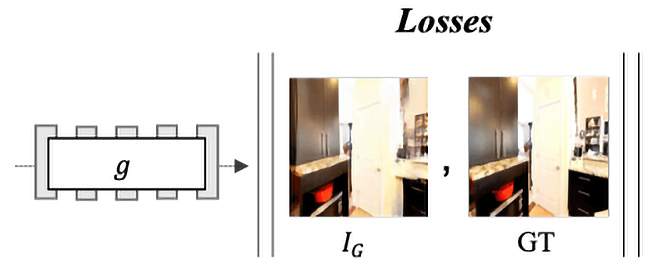
Figure 9.10: An example of the output of eval_kitti.py

The first image is the input image, and the second image is the ground truth. The third image is the network output. As you might have noticed, the camera was moved forward slightly, and for this specific case, the model output seems very well generated.

7. However, we need some numerical representation to understand how well the network works. That is why we need to run the evaluation/evaluate_perceptualsim.py file, which will calculate the accuracy:

   python evaluation/evaluate_perceptualsim.py

        --folder ${TEST_FOLDER}

        --pred_image im_B.png

        --target_image im_res.png

        --output_file kitti_results

The preceding command will help to evaluate the model given the path to test images, where one of them is the predicted image and the other one is the target image.

The output from my test is as follows:

Perceptual similarity for ./DATA/dataset_kitti/test_folder/:  2.0548

PSNR for /DATA/dataset_kitti/test_folder/:  16.7344

SSIM for /DATA/dataset_kitti/test_folder/:  0.5232

One of the metrics used in the evaluation is perceptual similarity, which measures distance in the VGG feature space. The closer to zero, the higher the similarity between images. PSNR is the next metric to measure image reconstruction. It calculates the ratio between the maximum signal power and the power of distorting noise, which, in our case, is the reconstructed image. Finally, the Structural Similarity Index (SSIM) is a metric that quantifies the deterioration in image quality.

8. Next, we can use a pre-trained model for inference. We need an input image that we will use for inference:

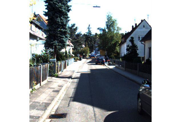
Figure 9.11: The input image for inference

9. Next, we will use the realestate model to generate a new image. First, we need to set up the model.

The codes for setting up the model can be found in the GitHub repository in a file called set_up_model_for_inference.py.

To set up the model, first, we need to import all the necessary packages:

import torch

import torch.nn as nn

import sys

sys.path.insert(0, './synsin')

import os

os.environ['DEBUG'] = '0'

from synsin.models.networks.sync_batchnorm import convert_model

from synsin.models.base_model import BaseModel

from synsin.options.options import get_model

10. Next, we are going to create a function that takes the model path as an input and outputs the model ready for inference. We will break the whole function into smaller chunks to understand the code better. However, the complete function can be found on GitHub:

          torch.backends.cudnn.enabled = True

          opts = torch.load(model_path)['opts']

          opts.render_ids = [1]

           torch_devices = [int(gpu_id.strip()) for gpu_id in opts.gpu_ids.split(",")]

           device = 'cuda:' + str(torch_devices[0])

Here, we enable the cudnn package and define the device on which the model will be working. Also, the second line imports the model, allowing it to gain access to all the options set for the training, which can be modified if needed. Note that render_ids refers to the GPU ID, which, in some cases, might be different for users with different hardware setups.

11. Next, we define the model:

    model = get_model(opts)

    if 'sync' in opts.norm_G:

    model = convert_model(model)

    model = nn.DataParallel(model,       torch_devices[0:1]).cuda()

    else:

        model = nn.DataParallel(model, torch_devices[0:1]).cuda()

The get_model function is imported from the options.py file, which loads the weights and returns the final model. Then, from options, we check whether we have a synchronized model, which means we are running the model on different machines. If we have it, we run the convert_model function, which takes the model and replaces all the BatchNorm modules with the SunchronizedBatchNorm modules.

12. Finally, we load the model:

    #  Load the original model to be tested

    model_to_test = BaseModel(model, opts)

    model_to_test.load_state_dict(torch.load(MODEL_PATH)['state_dict'])

    model_to_test.eval()

    print("Loaded model")

The BaseModel function sets up the final mode. Depending on the train or test mode, it can set the optimizer and initialize the weights. In our case, it will set up the model for test mode.

All this code is summed up in one function called synsin_model, which we will import for inference.

The following code is from the inference_unseen_image.py file. We will write a function that takes the model path, the test image, and the new view transformation parameters and will output the new image from the new view. If we specify the save_path parameter, it will automatically save the output image.

13. Again, we will first import all the modules needed for inference:

    import matplotlib.pyplot as plt

    import quaternion

    import torch

    import torch.nn as nn

    import torchvision.transforms as transforms

    from PIL import Image

    from set_up_model_for_inference import synsin_model

14. Next, we set up the model and create the data transformation for preprocessing:

    model_to_test = synsin_model(path_to_model)

        # Load the image

        transform = transforms.Compose([

            transforms.Resize((256,256)),

            transforms.ToTensor(),

            transforms.Normalize((0.5, 0.5, 0.5), (0.5, 0.5, 0.5))])

        if isinstance(test_image, str):

            im = Image.open(test_image)

        else:

            im = test_image

        im = transform(im)

15. Now we need to specify the view transformation parameters:

        # Parameters for the transformation

        theta = -0.15

        phi = -0.1

        tx = 0

        ty = 0

        tz = 0.1

    RT = torch.eye(4).unsqueeze(0)

    # Set up rotation

    RT[0,0:3,0:3] = torch.Tensor(quaternion.as_rotation_matrix(quaternion.from_rotation_vector([phi, theta, 0])))

    # Set up translation

    RT[0,0:3,3] = torch.Tensor([tx, ty, tz])

Here, we need to specify parameters for rotation and translation. Note that theta and phi are responsible for rotation, while tx, ty, and tz are used for translation.

16. Next, we are going to use the uploaded image and new transformation to get output from the network:

    batch = {

        'images' : [im.unsqueeze(0)],

        'cameras' : [{

            'K' : torch.eye(4).unsqueeze(0),

            'Kinv' : torch.eye(4).unsqueeze(0)

        }]

    }

    # Generate a new view of the new transformation

    with torch.no_grad():

        pred_imgs = model_to_test.model.module.forward_angle(batch, [RT])

        depth = nn.Sigmoid()(model_to_test.model.module.pts_regressor(batch['images'][0].cuda()))

Here, pred_imgs is the model output that is the new image, and depth is the 3D depth predicted by the model.

17. Finally, we will use the output of the network to visualize the original image, the new predicted image, and the output image:

        fig, axis = plt.subplots(1,3, figsize=(10,20))

        axis[0].axis('off')

        axis[1].axis('off')

        axis[2].axis('off')

        axis[0].imshow(im.permute(1,2,0) * 0.5 + 0.5)

        axis[0].set_title('Input Image')

        axis[1].imshow(pred_imgs[0].squeeze().cpu().permute(1,2,0).numpy() * 0.5 + 0.5)

        axis[1].set_title('Generated Image')

        axis[2].imshow(depth.squeeze().cpu().clamp(max=0.04))

        axis[2].set_title('Predicted Depth')

We use matplotlib to visualize the output. Here is the result of the following code:

Figure 9.12: Result of the inference

As we can see, we have a new view, and the model reconstructs the new angle very well. Now we can play with transformation parameters, to generate images from another view.

18. If we slightly change theta and phi, we get another view transformation. Now we will reconstruct the right part of the image:

      # Parameters for the transformation

        theta = 0.15

        phi = 0.1

        tx = 0

        ty = 0

        tz = 0.1

The output looks like this:

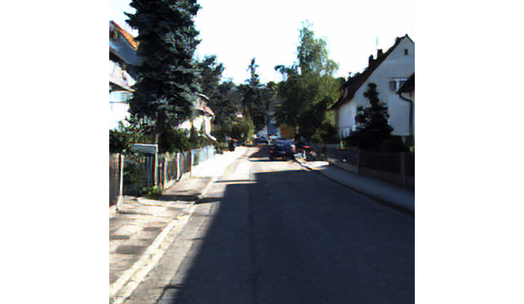
Figure 9.13: The result of the inference

Changing the transformation parameters all at once or changing them in bigger steps can result in worse accuracy.

19. Now we know how to create an image from the new view. Next, we will write some brief code to sequentially create images and make a small video:

    from inference_unseen_image import inference

    from PIL import Image

    import numpy as np

    import imageio

    def create_gif(model_path, image_path, save_path, theta = -0.15, phi = -0.1, tx = 0,

                  ty = 0, tz = 0.1, num_of_frames = 5):

        im = inference(model_path, test_image=image_path, theta=theta,

                       phi=phi, tx=tx, ty=ty, tz=tz)

        frames = []

        for i in range(num_of_frames):

            im = Image.fromarray((im * 255).astype(np.uint8))

            frames.append(im)

            im = inference(model_path, im, theta=theta,

                       phi=phi, tx=tx, ty=ty, tz=tz)

        imageio.mimsave(save_path, frames,  duration=1)

This chunk of code takes an image as input and, for the given number of frames, generates sequential images. By sequential, we mean that each output of the model becomes the input for the next image generation:

Figure 9.14: Sequential view synthesis

In the preceding figure, there are four consecutive frames. As you can see, it’s harder and harder for the model to generate good images when we try bigger steps. This is a good time to start playing with the model’s hyperparameters, different camera settings, and step sizes to see how it can improve or reduce the accuracy of the model’s output.

Summary

At the beginning of the chapter, we looked at the SynSin model structure, and we gained a deep understanding of the end-to-end process of the model. As mentioned earlier, one interesting approach during the model creation was a differentiable renderer as a part of the training. Also, we saw that the model helps to solve the problem of not having a huge, annotated dataset, or if you don’t have multiple images for test time. That is why this is a state-of-the-art model, which would be easier to use in real-life scenarios. We looked at the pros and cons of the model. Also, we looked at how to initialize the model, train, test, and use new images for inference.

In the next chapter, we will look at the Mesh R-CNN model, which combines two different tasks (object detection and 3D model construction) into one model. We will explore the architecture of the model and test the model performance on a random image.