Since so much scientific visualization starts with looking at underlying mathematics, we are beginning this book on 3D printing for science projects with a chapter on 3D printing mathematical functions. The basic models in this chapter are intended to be a starter set that you alter to 3D print whatever function you like, within the boundaries we will get to in a later section.
Math Modeling for 3D Printing
It seems like it should be easy to just put an equation into a program and have the printer “draw” it somehow, like some sort of 3D pen plotter. However, if a 3D printer head just tried to follow an equation, it would have no way of knowing how to avoid material that had already laid down, so we have to go about it in a bit more roundabout way.
3D Printing
3D printers require a several-step process from the first idea to a finished print. First, you need to develop a 3D model, as we will in this chapter. Models in this chapter (and most of the remainder of the book) are based on the free, open source 3D solid modeling program OpenSCAD (www.openscad.org). OpenSCAD allows you to encode geometrical models in a language that is sort of a subset of the C programming language. Good documentation is available by clicking the Documentation button on the OpenSCAD site’s home page.
Then, other software takes this model and slices it into layers, which the printer will then create one at a time, typically from the bottom up. We will use the open source MatterControl host program throughout this book, available free from www.mattercontrol.com. Appendix A talks more about things you should know about OpenSCAD, MatterControl, and 3D printing in general.
![]() Tip This book presumes you are generally familiar with 3D printing practices. If not, you can learn how to use a printer from Joan’s previous book, Mastering 3D Printing (Apress, 2014) or our book 3D Printing With MatterControl (Apress, 2015). Unless we specifically note otherwise, prints in this book were created on a Deezmaker Bukito in polylactic acid (PLA) plastic, using the MatterSlice engine in MatterControl (although we could have used any software compatible with an open source printer).
Tip This book presumes you are generally familiar with 3D printing practices. If not, you can learn how to use a printer from Joan’s previous book, Mastering 3D Printing (Apress, 2014) or our book 3D Printing With MatterControl (Apress, 2015). Unless we specifically note otherwise, prints in this book were created on a Deezmaker Bukito in polylactic acid (PLA) plastic, using the MatterSlice engine in MatterControl (although we could have used any software compatible with an open source printer).
Math Background
This chapter presumes you know what a function is—a relationship among a number of variables. In this case, we are dealing with functions using three variables, which we will call x, y, and z. Function notation looks like this: z = f (x,y). All that means is that our variable, z, can be computed for any given pair of values for the x and y variables. Having three variables means we can define shapes in three dimensions, with one variable corresponding to each dimension. Normally these three-dimensional shapes would be shown on a page with two-dimensional projections. Often, this is fine and you can see what is going on. Sometimes, however, it really helps to hold a 3D model in your hand and turn it this way and that. This chapter will give you the ability to do that for many types of functions.
![]() Note 3D printing convention holds that x and y are in the plane of the platform that your model is being built up on, and z is vertical height above that. In other words, the bottom of the surfaces generated in this chapter is always the z = 0 plane. In this convention, you always have to transform what you are printing to have z greater than or equal to zero, since you cannot build under the platform. In other words, if you know that z would be negative for some values of x and y that you want to use, you may have to add an offset to your equation so that z is always greater than zero and remember that the offset is there when you think about what your model represents.
Note 3D printing convention holds that x and y are in the plane of the platform that your model is being built up on, and z is vertical height above that. In other words, the bottom of the surfaces generated in this chapter is always the z = 0 plane. In this convention, you always have to transform what you are printing to have z greater than or equal to zero, since you cannot build under the platform. In other words, if you know that z would be negative for some values of x and y that you want to use, you may have to add an offset to your equation so that z is always greater than zero and remember that the offset is there when you think about what your model represents.
We will get you started with a model entirely in OpenSCAD that creates surfaces of functions z = f (x,y), where x and y are the plane of the 3D printer’s build platform, and z is the height of the surface above that plane. First we will show you how the basic 3D math model Rich has written and included here works, and what kind of functions you can print. Then we will show you a simple model that creates surfaces that might be a starting point for your own projects in OpenSCAD.
Alternatively you may have code you developed that produces a surface you would like to 3D print. It may not be practical to port that code to an OpenSCAD model. We will also show you an example in which we wrote a separate Python script that produces a file, which is then read into OpenSCAD and made into a surface. Finally we will give you some ideas about how you might use these tools as a teacher or as part of a student project.
Others (see links at “Where To Learn More” later in this chapter) have used more sophisticated mathematics modeling programs, but our desire here is to make this completely accessible and free so that you can get started without investing in software, at least at the beginning of your explorations.
Creating Surfaces Entirely in OpenSCAD
In this section we show you how to create a polynomial with a flat base. In the next section we show you what a print of a double-sided surface looks like using the same OpenSCAD code with different parameters. This model was written to be simple and easy to alter, which means that it does not check for complicated problems, like functions that go to infinity or other mathematically bad behavior. It does, however, let you input a function f (x,y) (as you can see in Listing 1-1). It uses OpenSCAD’s polyhedron module to accomplish this.
Making a Smooth Surface with a Flat Bottom
Listing 1-1 is the OpenSCAD model that creates a flat-bottomed “slice” of a surface, like a chunk cut out of a mountain range. The function in this example is z = f (x, y) = 0.01 (x – 50) (y – 50) + 30, and the 3D print will go from x = 0 to 99 and y = 0 to 99. This creates a “saddle point” structure, as shown in Figure 1-1. The model will create a surface xmax mm in x and ymax mm in y, with z height computed in mm. If the resulting structure is too big (by default, 99 mm by 99 mm on the bottom, or a bit less than 4 inches square), then you can scale the whole piece in your 3D-printing software. Figure 1-1 was scaled down to one-quarter scale.
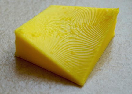
Figure 1-1. Saddle function with a flat bottom. Printed at quarter scale, so each side is about 25 mm, or just under an inch long. Layer height was 0.2 mm
The values of x and y go from 0 to xmax and ymax respectively. A maximum of 100 points in each dimension (xmax = 99 and ymax = 99) is allowed. The model will step in units of 1, which cannot be changed. If you want your model to step in smaller or larger increments, you will need to scale the variable in the equation.
For example, if in your original equation you had a function you wanted to increment by 0.02 in each step, replace the x in your original equation by (0.02 * x) to accomplish the same thing when you increment by 1. Or if you want to step from –500 to –400 in the original function, replace the x in your original function with (x – 500) everywhere to accomplish the same thing. Be careful if variables are raised to a power, or are inside a function like cosine, that you do this scaling correctly and consistently.
![]() Caution Because we are creating a flat bottom, the equation being represented here is actually 0 <= z <= f (x, y ). As a result, z = f (x, y) must be greater than zero everywhere for the flat-bottomed (thick = 0) version. A model will still be produced if there are z values that are less than zero, but it will be an invalid model, and even if you manage to repair it, it won’t print easily.
Caution Because we are creating a flat bottom, the equation being represented here is actually 0 <= z <= f (x, y ). As a result, z = f (x, y) must be greater than zero everywhere for the flat-bottomed (thick = 0) version. A model will still be produced if there are z values that are less than zero, but it will be an invalid model, and even if you manage to repair it, it won’t print easily.
![]() Note The OpenSCAD models in this book are written by Rich Cameron and licensed under a Creative Commons Attribution-NonCommercial-ShareAlike 4.0 International License—see http://creativecommons.org/licenses/by-nc-sa/4.0/ for details.
Note The OpenSCAD models in this book are written by Rich Cameron and licensed under a Creative Commons Attribution-NonCommercial-ShareAlike 4.0 International License—see http://creativecommons.org/licenses/by-nc-sa/4.0/ for details.
Printing Considerations
Since this model was designed to have a flat bottom, it prints easily. There will not be any overhangs. If your function would get very tall, you may want to scale it down by multiplying the equation by a constant. To check that the function is not getting too big or going negative in the z direction, you can either just run it in OpenSCAD and look at the result, or graph it conventionally yourself to see what it looks like. (The model does not check it for you.)
Limitations and Alternatives
To keep the model simple, transparent, and easy to understand, we have not inserted any error checking or special cases. Obviously, if you have a function that goes to infinity or has some sort of discontinuity, you will need to come up with some fix. You could, for example, create a branch in the definition of f (x, y) to handle cases that are poorly behaved in the mathematical sense.
We could only test a few cases, and there are an infinite number of options, so as with any print you should check the software model of your print before committing it to be sure that it worked for your particular example. As discussed earlier, z has to be greater than zero.
Another parameter in the code is blocky, which in this example is set to false. Setting blocky = true will create a slightly rough-textured surface instead of the smooth one here, which generally will take a lot longer to render in OpenSCAD—we have pulled out this code in a later section as a freestanding tiny model, so you might want to try using it that way.
![]() Caution OpenSCAD’s math functions will probably look familiar if you are a programmer, but some of them will not be what you are expecting if you do not have that experience already. Exponents, for example, take the form of pow(base, exponent) rather than using a superscript, and a square root uses the sqrt() function instead of a radical sign. You can find a (nearly) complete listing of the mathematical functions available in OpenSCAD at https://en.wikibooks.org/wiki/OpenSCAD_User_Manual/Mathematical_Functions.
Caution OpenSCAD’s math functions will probably look familiar if you are a programmer, but some of them will not be what you are expecting if you do not have that experience already. Exponents, for example, take the form of pow(base, exponent) rather than using a superscript, and a square root uses the sqrt() function instead of a radical sign. You can find a (nearly) complete listing of the mathematical functions available in OpenSCAD at https://en.wikibooks.org/wiki/OpenSCAD_User_Manual/Mathematical_Functions.
Making a Two-Sided Smoothed Surface
Although it is convenient to be able to visualize the top of a surface in 3D, sometimes it is even better to see it from both sides. However, you might think that then you will have to put a lot of support under the surface and wind up more or less with the same thing. The way out of this is to print the surface sideways. As long as the surface does not contain slopes that are too steep, you can use the following process to print a surface that is a few mm thick (2 mm in this example, the minimum we recommend) and print it on its side.
Run the same model in OpenSCAD as in the previous section (after changing the thick parameter to equal the desired thickness in mm), scale it if you like (be sure the thickness does not go below 2 mm), and rotate it 90 degrees about either the x or y axis. Look at your model to determine which rotation will have the fewest overhangs. If the excursions in f (x, y) were big, you might have to use some support this way but probably far less than if you laid the surface flat. As a bonus, z can be negative in this version.
![]() Tip For stability, it is wise to add some material to the platform in the first layer around the print. Your software may call this a brim; if you are not given the option of using a brim, use a skirt zero distance from the print instead, which is equivalent. Figure 1-2 shows the skirt in MatterControl; we told the software to use a five-loop skirt and to place it 0 mm away.
Tip For stability, it is wise to add some material to the platform in the first layer around the print. Your software may call this a brim; if you are not given the option of using a brim, use a skirt zero distance from the print instead, which is equivalent. Figure 1-2 shows the skirt in MatterControl; we told the software to use a five-loop skirt and to place it 0 mm away.
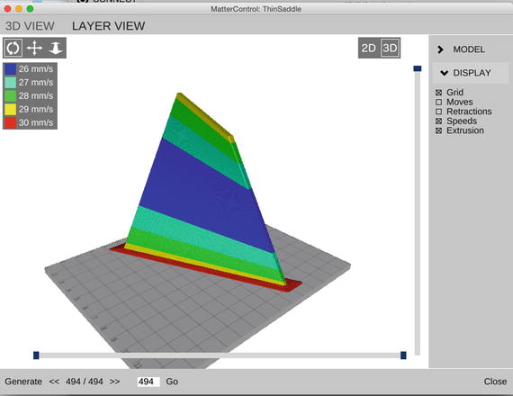
Figure 1-2. The simulated vertical version of the saddle surface in MatterControl. The brim is the wider are surrounding the first layer on the build platform. Shading (color in ebook) show different print speeds
The only difference between this case and the previous section is that the parameter thick was a nonzero positive number. In this case, we set it to 4. Thus, we generated a file that had the dimensions 99 by 99 mm in x and y, and was 4 mm thick in z. We decided that was bigger than we wanted to print, so we scaled down to half size in MatterControl (thus leaving it 49.5 mm by 49.5 mm by 2 mm thick.) Figure 1-3 shows the finished print still on the printer, held down in part by its attached skirt.

Figure 1-3. The saddle surface print as it finished
![]() Caution If you scale the surface, you have to be sure that the piece remains at least 2 mm or so thick after scaling. If you want something about 50 mm across, for example, and will be scaling it down by a factor of 2, you should start with thick = 4.
Caution If you scale the surface, you have to be sure that the piece remains at least 2 mm or so thick after scaling. If you want something about 50 mm across, for example, and will be scaling it down by a factor of 2, you should start with thick = 4.
Very Simple Model to Make a “Blocky” One-Sided Surface
Sometimes there are advantages to having a surface that is a bit rough. You might want to be able to feel the shape more, or you might want it to be a little more matte finish. The model in Listing 1-2 is an extremely simple one that will create an STL file with a surface of small cubical pieces. Rather than using triangular faces to interpolate as we did in the other model, this leaves the surface elements discretized. You are just creating xmax + 1 times ymax + 1 rectangular solids 1 mm by 1 mm by f (x, y) high. The blocky = true setting in Listing 1-1 produces the same result, but we have pulled it out and simplified it here for discussion purposes, and to give you something simpler to play with on your own. It is slower than the model in Listing 1-1 (with blocky = false) for most cases, but its very simplicity may give you some ideas of things you may want to try. Figure 1-4 shows a surface generated this way. OpenSCAD can take a while to render 100 by 100 surfaces this way.
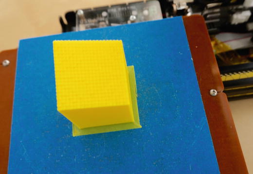
Figure 1-4. The blocky surface, as printed, scaled by 2 in the x and y direction, original scaling in z
Creating Surfaces from an External Data File
The processes we have used in the chapter so far have the virtue that everything was controlled entirely within OpenSCAD. However, since OpenSCAD does not have variables in the normal coding sense of the word, it is hard to do things like scale the surface dynamically or do any of the other things you might want to do for a complex mathematical model. (OpenSCAD has variables as a mathematician might think of them—what most programming languages would call constants.) You might have another piece of software creating your surface data points, and all you want to do is essentially plot them out as a 3D surface, either with a flat base or as a thin surface.
In this section, we use OpenSCAD’s surface module to plot a file of points generated by a program in the common language Python. There is nothing special about using Python versus C or any other language, but it does happen to be a language often used by scientists, so we felt it was appropriate here. The only critical thing is that the language needs to be able to create a text file in a format we will get to shortly. You could use a spreadsheet or for that matter a text editor to create your file of values.
Example: Using a Python Program to Generate Data for a Thin Surface
Listing 1-3 is a file Joan created in the Apple Python 2.7.8 Integrated Development Environment (IDE) that creates a 100 by 100 point matrix of two superposed radial cosine waves and stores it in the file sinusoids.dat. It is creating a file of datapoints for the surface
![]()
where r1 is a radial distance centered on x = 50 and y = 50 (1 mm from the center of Figures 1-5 and 1-6) and r2 is a radial distance centered on x = 0, y = 0 (defined as the lower right-hand corner of the pieces in this section). The offset of 6 ensures that the surface will always be at least 2 mm thick, since the other two terms are at a minimum a sum equal to –4.
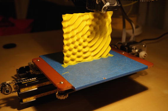
Figure 1-5. The model as it was being printed, showing the skirt (extra plastic where the object meets the build platform)
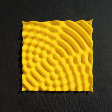
Figure 1-6. The model after it finished printing. (0, 0) is on the lower left
![]() Note There are many versions of Python available for free. If you want to look up the functions discussed so far, you can find good documentation at https://docs.python.org/2/index.html. Mac computers with OS X above version 10.3 come bundled with Python, and various free versions are available for Windows computers.
Note There are many versions of Python available for free. If you want to look up the functions discussed so far, you can find good documentation at https://docs.python.org/2/index.html. Mac computers with OS X above version 10.3 come bundled with Python, and various free versions are available for Windows computers.
The code in Listing 1-3 creates a file in the same directory as the code file. Then we created a model in OpenSCAD, which also had to run in the same directory. (We could have created a full directory path for it, but chose not to.) Listing 1-4 shows this model.
This says to print the data in the file sinusoids.dat and center the surface at (0, 0) and specifies a parameter that affects how the surface is viewed in OpenSCAD itself (without bearing on the final transformation into a printable file). Then we subtract away a surface 2 mm away, which leaves a surface 2 mm thick.
Constraints
The two surfaces have to have a clean 2 mm offset from each other or this does not work. The value of fxy in Listing 1-3 has to be greater than the offset value in Listing 1-4, so you will need to add an offset to fxy to keep it from going below the offset (here, the offset used was 2).
Figure 1-5 shows the model nearing completion (it was rotated so that (0, 0) wound up in the upper left, as seen there), and Figure 1-6 shows it completed. There was some stringing from lack of support in this orientation, but not disastrously so. If you had a surface that had a minimum value that was less obvious than the example just given, you could of course compute your points, find the minimum, and apply an offset such that every data point had a z value of at least the planned thickness of the surface. In this example, we are creating a surface that is 100 mm by 100 mm and 2 mm thick. If the z value is less than that, one side of the surface may be clipped when you print it.
![]() Note The format that OpenSCAD expects for its surface function is a text file with values in a row separated by spaces, with a newline at the end of each row. OpenSCAD’s surface module will create a shape using the z values from the file in a 1mm grid, just like that in Listing 1-1. Values need to be greater than zero for reliable results.
Note The format that OpenSCAD expects for its surface function is a text file with values in a row separated by spaces, with a newline at the end of each row. OpenSCAD’s surface module will create a shape using the z values from the file in a 1mm grid, just like that in Listing 1-1. Values need to be greater than zero for reliable results.
THINKING ABOUT THESE MODELS: LEARNING LIKE A MAKER
In each chapter of this book, we will talk a little about what we learned while we were developing the models, so that you can think a little about what you would like to do with them. This chapter is a little different from the rest in that the models here are an underlying tool that is useful for many of the other chapters of the book. In Chapter 2, for example, we will explore waves and fields, and will draw on the ability to plot out 3D functions that are usually shown as 2D projections.
In our case, we had to think hard about what types of functions would most usefully be visualized this way and how to balance an overly complex model that would be hard for you to alter versus a reasonably capable one. After a lot of experimentation, we came up with the set described here. We encourage you to play with them and let us know what else you come up with. (See Appendix A for information about how to contribute to the open source repository of these models.)
Finally, we have been surprised at how much mathematical insight comes about through first thinking about how to create the model and then handling the finished product. Just flipping over a sinusoid (as in the last example) leads you to ask a lot of questions about how the different sinusoidal functions are related.
We found as we worked on some of the models later in this book that often everyone uses the same 2D projection of a 3D model, and that actually creating the entire model literally gives you a different perspective. Figure 1-7 shows all the objects in this chapter together. It is a bit of an exercise in seeing how different a 2D photograph can make a 3D surface look; with the models in hand, we really struggled to arrange them to make it clear what shape they were and what the scale of any imperfections was, relative to the object itself.
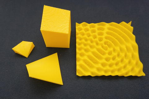
Figure 1-7. All the models from this chapter together for comparison
Where to Learn More
There are obviously many different sites to learn about the mathematics of the example functions shown in this chapter. Joan’s personal favorite place to send students to learn more about math (but not tied to 3D printing) is the Kahn Academy, at www.khanacademy.org.
If you want to see some other 3D-printed mathematics, have a look at the sites of Elizabeth Denne (of Washington and Lee University), which mostly use Mathematica for modeling:
http://mathvis.academic.wlu.edu
http://home.wlu.edu/~dennee/math_vis.html
http://www.thingiverse.com/dennedesigns/about
Sculptors Bathsheba Grossman and Henry Segerman create mathematics-based sculpture, available at their respective sites www.bathsheba.com and www.shapeways.com/shops/henryseg. Paul Nylander (http://bugman123.com) has a variety of math- and science-oriented models on his site. And of course, you can always search on the various websites of 3D models (such as www.thingiverse.com/explore/newest/learning/math and www.youmagine.com) for math models.
Teacher Tips
In later chapters, we give some suggestions about alignments to science standards. Here, rather than give an enormous list of possible links, we will just note that pretty much any level of math that can benefit from tactile demonstrations can be served by prints created by this software, and the science that uses that mathematics can benefit similarly. (For example, in Chapter 2 we show how to use some of these surfaces to visualize light waves and gravity fields.)
We intended these model for surfaces that are difficult to visualize and that can be hard to think about in projected form, but you may find someone in one of your classes at any level who will find a 3D model can break a logjam. At the simplest level, you can print out sample functions with a few parameters changed and have durable visualization tools that can survive being passed around a classroom.
Science Fair Project Ideas
If you decide you want to have a 3D-printed mathematical function as part of a project, you will discover that you think differently about a math function when you are considering how to display it in 3D versus using the same 2D illustration that everyone else uses. Consider, for example, printing out a model of a function that applies to your product and taking measurements off it with a pair of calipers to see whether it agrees with theory. See if the creation of the physical model and any issues you had while printing give you insight into the problem.
Summary
In this chapter, you learned several different ways to create a 3D model of a mathematical function in the OpenSCAD 3D solid modeling program, either one-sided on a flat base or as a thin two-sided sheet. You also saw how to create a file with an external program (Python code in the example) to pass through OpenSCAD, in case you are generating surfaces in other codes and would like 3D models of them. Finally, we gave you a few pointers to places to see more math examples and some ways to use these models in teaching and science fairs.