
When someone says “waves,” the first thing that may come to mind is the kind of waves that crash onto a beach. Water waves (and waves in air) are actually pretty complicated, because the waves are moving over complex terrrain, experiencing friction and effects of the water’s viscosity and a lot of other things. The equations that govern water waves and the interactions among them require that you know about a type of math called partial differential equations, which even scientists and engineers might not work with much until graduate school.
Fortunately, though, light waves and other electromagnetic radiation follow some rules that simplify a lot of things for some special cases. The geometries of even these simpler interacting wave examples can be pretty complicated, though. In this chapter, we will develop some 3D-printable models that represent some of these special cases to help you visualize wave interactions. Students at all levels have trouble visualizing the properties of light and magnetism because of their abstract nature; if you are a teacher, you may find some of these materials useful just to pass around while discussing some of these phenomena.
This chapter assumes you are pretty comfortable with trigonometric functions like sine, cosine, and tangent and their inverses (asin, acos, atan). We also talk about the sinc(x) function, which is just sinc(x) = sin(x)/x, defined as equal to 1 if x = 0. (Since 0/0 is always “undefined” mathematically, a definition is needed for the function to have a value right at x = 0—otherwise it would approach 1 as x got small, but never quite get there.) Some types of engineers define sinc(x) differently, so be sure you are using the one shown here.
We will explore some topics that are typically taught at levels from high school through the research level, and the eager student will have a lot of places they can go exploring further. (The authors would like to acknowledge the assistance of astronomer and interferometry expert Stephen Unwin in clarifying the physics underlying this chapter and suggesting good ways to frame some of the basics without resorting to calculus.)
![]() Note Everything in this chapter is generated with OpenSCAD for modeling and MatterControl for controlling the printer. The demonstration prints illustrated in this chapter were done on a Deezmaker Bukito printer, using PLA plastic, with 0.2 mm layer height and no support other than a brim (or attached skirt, if you prefer to think of it that way) to glue down the first layer.
Note Everything in this chapter is generated with OpenSCAD for modeling and MatterControl for controlling the printer. The demonstration prints illustrated in this chapter were done on a Deezmaker Bukito printer, using PLA plastic, with 0.2 mm layer height and no support other than a brim (or attached skirt, if you prefer to think of it that way) to glue down the first layer.
Physics and Math Background
The models in this chapter are two-dimensional waves (in the x/y plane). We show their amplitude as the model’s height in the z direction. In the case of a water wave, the height of the water wave would be the z value. For a light wave, it is better to think of the height (value of z) as the brightness of the light at that x, y position at a snapshot in time. In some other cases, we will calculate the square of the amplitude and display that as the z value. That can be thought of as the average over time of the waves passing through that point in space, since the waves are propagating over time. We show them in the models in this chapter as just functions of space—a snapshot at a particular time, or an average over time, as the case may be.
Coordinate System and Conventions
For all the models in this chapter, we used xmax and ymax set to 99 (see Listing 1-1 ). This means that the models are all 100 by 100 points and by default will print out 100 by 100 mm (about 4 inches square, with thickness depending on other parameters that we describe for each case). More points are usually better, but more points can make the OpenSCAD model take a very long time to render and require you to do some scaling down unless you have a very big printer. This value seems to be a good tradeoff that keeps feature size big enough to be printed while preserving the important features. You will need to play with this a little as you develop models.
The origin is at the lower right-hand corner, and x and y are both always positive and go from 0 to 99. Some of the models add an offset to the z value to make printing possible (since 3D printers usually have a convention that z = 0 is the printer’s build platform, so nothing can be printed with a negative z value).
As we will talk about later in the chapter, we will not normally 3D print these models such that the x and y axes of the models are printed aligned with the x and y plane (parallel to the build platform) of the 3D printer. When we talk about x, y, and z in this chapter, we mean the coordinates of the model.
Finally, OpenSCAD uses degrees in its trigonometric functions. In most of our illustrations, we talk about angles in radians, since that is how most textbooks present the problems, and also because it works out conveniently in many more advanced topics, should you choose to keep going. We note conversions as we go.
![]() Note We replaced the function f(x,y) used in Listing 1-1 to generate the models in this chapter. We give you just the model for the function (sometimes, several interrelated functions) in this chapter to avoid repeating the same model over and over. The downloadable model versions include the entire model in each file, incorporating both the function f(x,y) here plus the rest of the Listing 1-1 material. Comments in the model and shown here may vary somewhat for clarity and context.
Note We replaced the function f(x,y) used in Listing 1-1 to generate the models in this chapter. We give you just the model for the function (sometimes, several interrelated functions) in this chapter to avoid repeating the same model over and over. The downloadable model versions include the entire model in each file, incorporating both the function f(x,y) here plus the rest of the Listing 1-1 material. Comments in the model and shown here may vary somewhat for clarity and context.
Principle of Superposition
Imagine that you are on a still pond and you start poking a stick in and out of the water. Ripples will spread across the pond. Then suppose a friend nearby started doing the same thing. The ripples going in multiple directions would in some cases add up (creating a doubly-high ripple) and in others, subtract or cancel out.
In real life, the waves on the pond will die out and have other complex interactions, but we can get a lot of insight into many kinds of electromagnetic waves (like light and radio waves) by modeling the waves as simple sine and cosine waves that interact with each other like the ripples you just imagined on the pond.
For many kinds of waves, you can add the effects of the different waves, called the principle of superposition (https://en.wikipedia.org/wiki/Superposition_principle). When the waves add, it is called constructive interference; when they cancel each other out, it is destructive interference. We will use this principle, and an adaptation of the model from Listing 1-1, to visualize some classic experiments.
Some Basic Examples
To give you some feel for how different types of wave geometries might play out, we walk through a couple of examples. One of the things that this model makes very easy is putting together fairly complex combinations of sinusoids and seeing the wave interactions. As discussed later in the chapter, we will be simplifying some of the physics behind some of the wave phenomena we model, but you can still gain some good insight from playing with these models.
Point Sources and Plane Waves
This section looks at point sources, which put energy into a system in a concentrated way—sort of like the stick in the water we talked about earlier, or a small bright light in a big room. Energy from that source would then go out in all directions radially from the point. The other basic type of wave we talk about is a plane wave—a straight line wave across the whole plane, like waves far out at sea. Then we look how these appear when they are superposed on each other.
Listing 2-1 gives the OpenSCAD model for an overlap of the two types of waves. The plane wave has four times the amplitude of the radial source, and a wavelength five times as long. In Figure 2-1 you can see what a snapshot of this looks like when 3D printed. The print is 100 mm square and 3 mm thick. The waves going from left to right (that is, traveling in the x direction) are bigger and farther apart than the short ripples from the point source on the left, which is centered at the point (49.5, 49.5).
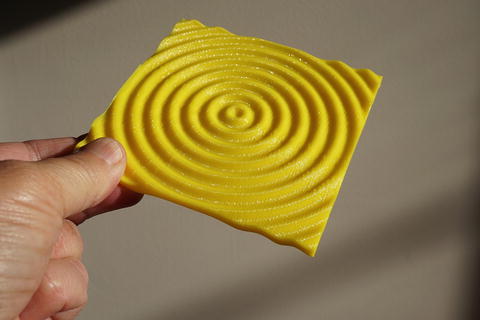
Figure 2-1. Just the point source radiating from the center
The model assumes that you are calculating a value for the combined waves at each point (x,y) on a square grid going from (0,0) to (99,99). However, many of the functions are in terms of the distance from a source to a particular point in space. We calculate that distance in the function radius, which calculates the distance from the source at (xc,yc) to the point (x,y). Figure 2-1 shows just the point source; Figure 2-2, just the plane wave; and Figure 2-3, the two superposed.
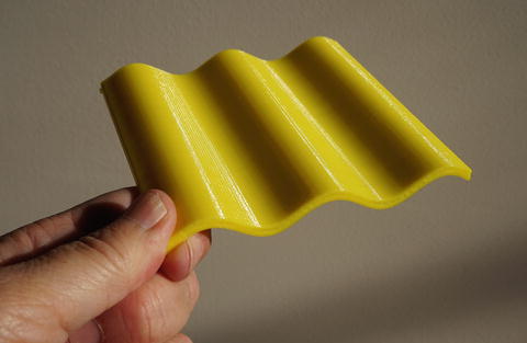
Figure 2-2. The plane wave alone
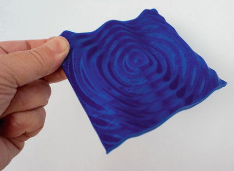
Figure 2-3. Plane wave and point source interaction
![]() Note OpenSCAD assumes degrees in all its trigonometric functions, and here radians are far more convenient. 2π radians = 360 degrees. This requires multiplying by 2π/360, or π/180, quite often in what follows. We show the equations in the form that assumes radians, since it is much simpler to understand. The two waves being superposed in Listing 2-1 are calculated in degrees. In radians, the first term would be cos(5r/6) and the second term, 4*sin(r/6).
Note OpenSCAD assumes degrees in all its trigonometric functions, and here radians are far more convenient. 2π radians = 360 degrees. This requires multiplying by 2π/360, or π/180, quite often in what follows. We show the equations in the form that assumes radians, since it is much simpler to understand. The two waves being superposed in Listing 2-1 are calculated in degrees. In radians, the first term would be cos(5r/6) and the second term, 4*sin(r/6).
Two Interacting Sources
What happens if we have two interacting point sources at one edge of the plane we are modeling? The model for that is given in Listing 2-2, and the model we printed is in Figure 2-4. In this case, we are printing a model in which z represents the square of the amplitude of the sum of the waves generated by these two sources. As we will see in the next section, this is also an equivalent of the time average of the intensity pattern that would be generated by a wave passing through two infinitely thin, infinitely long slits oriented at right angles to the print and located at x = xc1 and xc2. In the next section, we will see what happens when they are not infinitely thin slits.
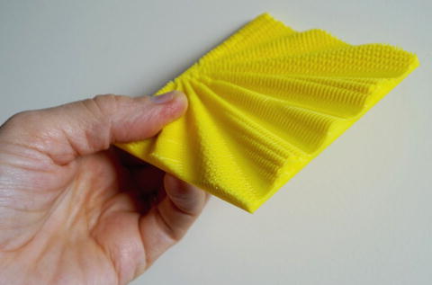
Figure 2-4. The square of the combined amplitudes of two point sources sending out waves radially on one plane, with a wavelength of 4 mm. The (0,0) point is on the upper right; the sources are just above the person’s thumb, on the edge of the model
In Listing 2-2, lambda is the wavelength, in mm; r is the distance (also in mm) from the center of each of the point sources to the point (x,y) on the surface; and factor is an arbitrary scaling factor to adjust how large the features are. Note that the equations are in radians because that is how they are shown in most physics books, but since OpenSCAD uses degrees, we needed to convert from the equation to its encoding.
We would need to use some calculus concepts to prove this, but generally speaking, the square of the amplitude is proportional to the average amplitude of a wave moving over a surface over time. We will use that smoothed average in the next section, so we do it here as well so that we can compare the results later.
![]() Note Raising a variable to a power in OpenSCAD uses the pow function, so pow(x,2) would return x squared.
Note Raising a variable to a power in OpenSCAD uses the pow function, so pow(x,2) would return x squared.
![]() Caution Some of the fine structure in Figure 2-4 is just an artifact of the sampling rate being too low for the given wavelength. We are sampling (creating a surface data point) every 1 mm, and the wavelength is only 4 mm. Given the averaging used in the model that creates the surface, this is not quite enough. We created this for comparison with later discussions of two finite slits. The finite slit case is a function of a particular angular maeasurement (and is not a snapshot in time as these are) and is not as vulnerable to these issues. Figure 2-5 shows the same surface with a wavelength four times as long (and sources 36 mm apart instead of 20).
Caution Some of the fine structure in Figure 2-4 is just an artifact of the sampling rate being too low for the given wavelength. We are sampling (creating a surface data point) every 1 mm, and the wavelength is only 4 mm. Given the averaging used in the model that creates the surface, this is not quite enough. We created this for comparison with later discussions of two finite slits. The finite slit case is a function of a particular angular maeasurement (and is not a snapshot in time as these are) and is not as vulnerable to these issues. Figure 2-5 shows the same surface with a wavelength four times as long (and sources 36 mm apart instead of 20).
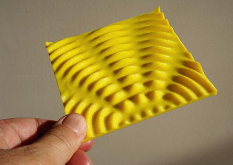
Figure 2-5. Longer wavelength version of Figure 2-4, with slits farther apart
More Complex Examples: Diffraction
We can combine some of these ideas to create some models of the phenomenon of diffraction (https://en.wikipedia.org/wiki/Diffraction). Waves diffract, changing their geometry and how they interact with each other when they encounter a physical barrier of some kind. What happens when a wave front passes through a wall with either one or two slits in it and contines through on the other side? In 1803 Thomas Young performed his double-slit experiment to try and quantify what the pattern of bright and dark areas would be if someone were to hold up a screen after the light had passed through these slits (see https://en.wikipedia.org/wiki/Young’s_interference_experiment for more). A note, though: here we are showing a monochromatic (one wavelength of simulated light) version of the experiment. The original experiment used multiple wavelengths and produced a rainbow interference pattern.
The Double-Slit Experiment
Figure 2-6 shows the setup of Young’s double-slit experiment, arranged the way we will refer to the various aspects of it in this section. The two slits are assumed to be larger than the wavelength of the light passing through them, close together relative to the overall area we are modeling. The angle θ is the angle between a light ray to a given point (x,y) and the vertical. A light wave from a source below the bottom of Figure 2-6 would shine through the two slits and then interact.
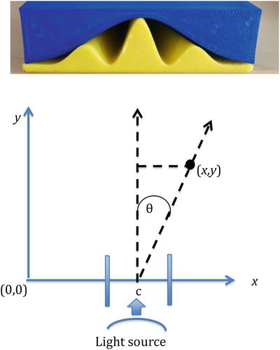
Figure 2-6. The double-slit experimental setup, along with some of the models from this chapter
Young found that what he saw were alternating light and dark bands on a screen behind his slits, showing how the wave front going through each slit interfered constructively and destructively at different points in space. This experiment was taken as proof that light travels in waves that can be added together to produce interference patterns. How the high and low areas of our 3D-printed models line up with the experiment’s geometry is shown in Figure 2-3 (except that the amplitude would be in the z direction, out of the page.)
One-Slit Examples
Light passing through just one slit in a similar setup gives a spread-out illuminated area after the light passes through the slit. For one slit, the equation for the intensity is proportional to sinc2(π d sinθ/λ) and for two slits, to cos2(π b sinθ/λ) sinc2(π d sinθ/λ); sinc(x) is defined as sin(x)/x unless x = 0, in which case sinc(0) = 1. Here d is the width of each slit, b is the distance between them, λ (the Greek letter lambda) is the wavelength, and θ (Greek letter theta) is the angle defined in Figure 2-6. This works out to the two-slit intensity being the intensity pattern from one slit multiplied by a (squared) cosine wave.
If you look at the models in Figures 2-7 and 2-8 you can see these patterns. We created a “negative space” version of the one-slit case so we could explore how well it fits over the two-slit case. In Figure 2-8 you can see that it does indeed fit pretty well. OpenSCAD functions for each of the objects shown in Figure 2-8 are in Listing 2-3 (two slits), Listing 2-4 (one slit), and Listing 2-5 (one-slit negative space).
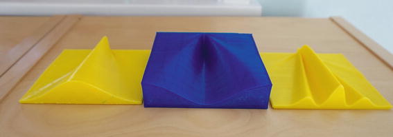
Figure 2-7. Model of light through one slit (positive, left, and inverted, center) and two slits (right). Illumination at the top as shown here
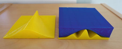
Figure 2-8. One-slit intensity function (left) and the negative-space version over the two-slit one
In Listing 2-4 we have a function sintheta(x,y). This function computes the sine of the angle theta (θ) from the geometry. Do not be confused by the lack of a call to the sin() function. Here we just go back to sine being opposite over hypoteneuse, as shown in in Figure 2-6.
![]() Caution In these models we cheated a little by avoiding situations where we would need to compute sinc(0), which is defined as equal to 1. (It is 0/0 otherwise.)
Caution In these models we cheated a little by avoiding situations where we would need to compute sinc(0), which is defined as equal to 1. (It is 0/0 otherwise.)
Figure 2-9 gives a top view of the one-slit intensity pattern (inverted, top left; positive, bottom left), the double-slit (top right), and the two infinitely thin slits spaced the same as the finite ones (bottom left). In all cases, they were printed with thick=0 (flat bottoms). The equations used are far field equations (known as Fraunhofer diffraction) and do not really apply right at the slits. You see some artifacts if you look closely.
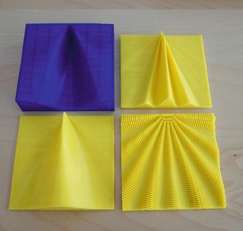
Figure 2-9. Inverted one slit (top L), two slits (top R), one slit (bottom L), and two point sources spaced the same as the slits and using the same wavelength (bottom R)
Applying this phenomenon for useful purposes is called interferometry. It has many applications in fields ranging from astronomy to manufacturing; we discuss some of them in the “Where to Learn More” section later in this chapter.
Printing Considerations
You may have been wondering how we were 3D printing the wave patterns when thick was not equal to zero (that is, when we did not have a flat bottom). Actually, all the objects in this chapter have been printed sideways. Figure 2-10 shows two of the objects (that did have thick=0) as they were printed. Depending on the orientation that will have the fewest overhangs, you may want to rotate the object in x or y plus or minus 90 degrees to get to this point.
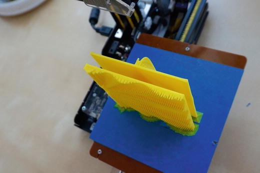
Figure 2-10. The infinitely thin pair of slits and the two finite slits printing at the same time
The other advantage of printing these functions vertically is that fine detail will print much better. If you had details with a lot of gaps between them, like the two point sources example (back in Figure 2-2), you will get a lot of stringing if you try to print a layer with a lot of gaps. But printing it vertically means that each layer essentially has no gaps on the surface perimeter, and just internal ones for the infill layers.
The print will stick well if you use a skirt that has four or five loops around the base, and is zero distance away, equivalent to a brim (different 3D-printing software refers to these differently.) You may want to have a wider and slower first layer extrusion.
THINKING ABOUT THESE MODELS: LEARNING LIKE A MAKER
When we started working on this chapter, we found ourselves asking a lot of fundamental questions about what we were trying to represent, and which models would give the most insight. One of the challenges here was that waves normally propagate in space and time, so in some ways a 3D model has the same issues as a 2D video simulation. You have three dimensions, but either it has to be a snapshot in time or one of the spatial axes needs to represent something other than the third dimension. Thinking about that and when it is worthwhile to have a “two-sided” model took a lot of time and discussion with several physicists.
In the “Science Fair Project Ideas” section later in this chapter, we talk about magnetism and why we decided not to include any models of magnetic fields. Magnetic fields were more difficult to think about in many ways because the magnetic fields have both a magnitude and a direction, which is difficult to show in a 3D static model. We explored models of simple bar magnets, as well as those of Earth’s magnetic field and of the Sun. However, very few simple equation solutions give very much insight, and many field equations are in very inconvenient (for 3D printing) polar coordinate systems. Others are designed for a static simple case that gives one number—not a very interesting 3D print.
A little digging revealed that as a practical matter many people who actually need to model these things rely on one of several semi-experimental models. It seemed to us like there were not a lot of models for which a surface without directional markings would be an improvement to a 2D drawing with arrows showing the field direction. However, we included it in the “Science Fair” section so that more advanced students might consider whether a simplified model, applied thoughtfully, might be interesting to explore a narrow hypothesis.
One of the things that came up with the set of models for this chapter was the idea of an envelope model. You could see pretty easily that the two-slit pattern fit inside the envelope created by the one-slit case, but creating a “negative space” model so that the two could actually be fit together was really interesting. We encourage you to think about other applications of this and places where it might give you more insight. Basically all you do is subtract the function of interest from a number big enough so that the negative space “fits inside” an outer box; see Figures 2-7 through 2-9 and Listing 2-5.
Because we elected not to use any math here beyond high school–level geometry and trigonometry, some of the discussion of the amplitude of the waves or why you may want to look at the square of the amplitude for a time average are of necessity a little vague and ignore some dependencies on time, frequency, and other things that are important in real applications. If you need to go beyond these rough conceptual ideas, be sure you know the equations governing your case and when the simplistic approach here is appropriate and when it is not.
Where to Learn More
Good general background on the topics in this chapter can be found at the Khan Academy (www.khanacademy.org/science/physics/light-waves) and many articles on Wikipedia. A good introductory college-level physics or electrical engineering textbook will help for the next level of exploration beyond what we have here.
The material in this chapter could be taken many different directions. We have not even touched on the many electrical engineering applications of Fourier Transforms, a technique that uses the mathematics of combining waves to solve engineering problems (https://en.wikipedia.org/wiki/Fourier_transform).
The properties of interfering waves are used routinely in applications that require a lot of precision. Astronomers use radio interferometry to create images of objects that, as they would say, subtend a small angle in the sky. This can either be something small that is sort of far away, or something big that is very, very far away. Astronomers make interferometry observations by taking signals from two radio telescopes (those big dishes like those seen in the movie Contact, for instance) and thinking of the two telescopes as two slits admitting light from a point source very far away (in this case, it might be another galaxy).
The farther away the telescopes are from each other, the finer the detail of the object that can be taken from the radio waves. If there are groups of telescopes at different distances from each other, an image can be built up from the signals of different resolution of the same object. The VLA (Very Large Array, www.vla.nrao.edu) in Socorro, New Mexico, was designed for this application with 27 radio telescopes arranged in a Y-shaped configuration.
A nearer-to-home application is laser interferometry for precise measurement of optical and other precision surfaces that are being machined. Laser beams interfere with each other when the surface is shaped correctly, and so the pattern from a test beam and one reflecting off the surface will give information about surface inaccuracies.
Teacher Tips
Waves in fluids are taught at various points in the K-12 curriculum. Light waves are dealt with in a somewhat cursory way, since as noted earlier many properties of waves cannot be fully appreciated until students have had some exposure to undergraduate-level physics and math.
However, playing with these models to build some intuiton can motivate learning about some of the precursor material or lead to science-fair or extra-credit projects. That said, if you enter “waves” on the Next Generation Science standards website (www.nextgenscience.org) you will get a lot of hits. Here are some we thought might be particularly good places to use the models here, or develop your own:
www.nextgenscience.org/msps-wer-waves-electromagnetic-radiation
www.nextgenscience.org/hs-ps4-3-waves-and-their-applications-technologies-information-transfer
www.nextgenscience.org/4-ps4-1-waves-and-their-applications-technologies-information-transfer
If you are developing curriculum based on these standards, we encourage you to search around and see if you can invent new 3D-printable models that build on the ones in his chapter. As with Chapter 1, we hope this chapter is a starter set that will give you ideas for your own projects.
Science Fair Project Ideas
Precisely because these concepts fairly rapidly lead into some sophisticated areas, we can imagine science fair projects that involve designing and printing a variety of different types of waves to compare, contrast, and measure. It seems to us that some interesting exercises could be built around one function being the envelope or negative space of another.
More Wave Interaction Models
If you know that a complex function can be approximated by summing sine waves of different frequency and amplitude, you can experiment a bit in OpenSCAD and then print out the ones that look particularly interesting or that you would like to try comparing or fitting into one another. For rapidly variable functions, be careful of the undersampling issues mentioned earlier. The way the model is designed, you can put in more points, though they will still be 1 mm apart (but the piece will get bigger). You can scale a 3D print in MatterControl or other 3D printer slicing software if the piece gets too big for your printer.
Magnetism Explorations
As mentioned at the beginning of the chapter, the full equations that govern the wave motions of light are complex partial differential equations. Light waves are part of the broader category of electromagnetic waves. The physics of light waves and magnetism are tied together with Maxwell’s equations (https://en.wikipedia.org/wiki/Maxwell’s_equations), which do not lend themselves to simple solutions in OpenSCAD.
Magnetic fields have the additional representational problem that they are directional. The simplest example of this is a bar magnet, with its north and south poles. Typically people show magnetic field lines by sprinkling iron filings around a magnet and then noting north and south poles of the magnet. This seemed to us to be a case where adding a third dimension did not add a lot to the discussion, since a two-dimensional slice through a field with directional arrows in some ways is more information than a three-dimensional surface might be.
People who actually have to model Earth’s magnetic field for navigational or other purposes resort to one of several semi-experimental models that are available. The Earth’s field is “blown back” heavily by the solar wind—charged particles released from the Sun. The solar wind varies over time, and this variation is known as space weather.
The Sun’s own magnetic field has some interesting interactions and also has semi-experimental models. One commonly used model is based fundamentally on an ancient mathematical construct called an Archimedes spiral. This model (https://en.wikipedia.org/wiki/Heliospheric_current_sheet) is referred to as the Parker Spiral after its originator.
We created some simple models that looked like magnetic fields, but after some debate we decided that the models were too simplistic and could lead readers to draw some incorrect conclusions about the more-complete mathematics. Making them “more right” would have taken us places that we felt were beyond the intended audience for this book and the desire to use simple and open source tools wherever possible. Thus we have decided not to include any magnetism models here, but we encourage advanced students and their teachers to think about what magnetic field line or potential surface models would be good for more insight. Exploring a special case or narrow application might lead to some interesting areas to explore.
Summary
This chapter developed some 3D-printable models of interacting sinusoidal waves, which are useful for modeling the physics of light, magnetism, and other phenomena. In particular, we learned about what happens when some different types of waves interact and how a light wave behaves after it passes through one or two thin slits. We learned some 3D-printing techniques (such as printing a thin object with a lot of detail on its side) and some modeling techiques (combining “negative space” models with conventional positive ones). Finally we gave various ideas for topics that could be taught with these models at grade levels from middle through graduate school.