8
Semantic Correspondences
8.1 Introduction
The approaches presented so far for shape correspondence are geometry driven, focusing solely on the geometrical and topological similarities between shapes. However, in many situations, corresponding shape parts may significantly differ in geometry or even in topology. Take the 3D models shown in Figure 8.1. Any human can easily put in correspondence and match parts of the chairs of Figure 8.1a despite the fact that they differ significantly in geometry and topology. For instance, some chairs have one leg while others have four. In these examples, correspondence is simply beyond pure geometric analysis; it requires understanding the semantics of the shapes in order to reveal relations between geometrically dissimilar yet functionally or semantically equivalent shape parts.

Figure 8.1Partwise correspondences between 3D shapes in the presence of significant geometrical and topological variations. (a) Man‐made 3D shapes that differ in geometry and topology. The partwise correspondences are color coded. (b) A set of 3D models with significant shape differences, yet they share many semantic correspondences.
This fundamental problem of putting in correspondence 3D shapes that exhibit large geometrical and topological variations has been extensively studied in the literature, especially in the past five years 183, 203–205. Beyond standard applications, such as blending and morphing, this problem is central to many modern 3D modeling tools. For instance, the modeling‐by‐example paradigm, introduced by Funkhouser et al. 206, enables the creation of new 3D models by pasting and editing 3D parts retrieved from collections of 3D models. Its various extensions 204, 207, which lead to smart 3D modeling techniques, create new 3D shape variations by swapping parts that are functionally equivalent but significantly different in geometry and topology.
In this chapter, we review some of the methods that incorporate prior knowledge in the process of finding semantic correspondences between 3D shapes. We will show how the problem can be formulated as the optimization of an energy function and compare the different variants of the formulation that have been proposed in the literature. We conclude the chapter with a discussion of the methods that are not covered in detail and outline some challenges to stimulate future research.
8.2 Mathematical Formulation
Let ![]() and
and ![]() be two input 3D objects, hereinafter referred to as the source and target shapes, respectively. The goal of correspondence is to find for each point on
be two input 3D objects, hereinafter referred to as the source and target shapes, respectively. The goal of correspondence is to find for each point on ![]() its corresponding point(s) on
its corresponding point(s) on ![]() , and for each point on
, and for each point on ![]() its corresponding point(s) on
its corresponding point(s) on ![]() . This is not a straightforward problem for several reasons. First, this correspondence is often not one‐to‐one due to differences in the structure and topology of shapes. Consider the example of Figure 8.1a where a desk chair has one central leg, a table chair has four legs, and the bench, which although has four legs, their geometry and structure are completely different from those of the table chair. Clearly, the one leg on the source chair has four corresponding legs on the target chair. Second, even when the source and target shapes have the same structure, matching parts can have completely different topologies (e.g. the backrests of the seats in Figure 8.1a), and geometries (e.g. the heads in the objects of Figure 8.1b). Thus, descriptors, which are only based on geometry and topology, are not sufficient to capture the similarities and differences between such shapes.
. This is not a straightforward problem for several reasons. First, this correspondence is often not one‐to‐one due to differences in the structure and topology of shapes. Consider the example of Figure 8.1a where a desk chair has one central leg, a table chair has four legs, and the bench, which although has four legs, their geometry and structure are completely different from those of the table chair. Clearly, the one leg on the source chair has four corresponding legs on the target chair. Second, even when the source and target shapes have the same structure, matching parts can have completely different topologies (e.g. the backrests of the seats in Figure 8.1a), and geometries (e.g. the heads in the objects of Figure 8.1b). Thus, descriptors, which are only based on geometry and topology, are not sufficient to capture the similarities and differences between such shapes.
One approach, which has been extensively used in the literature, is to consider this correspondence problem as a semantic labeling process. More formally, we seek to assign labels to each point on ![]() and
and ![]() such that points that are semantically similar are assigned the same label
such that points that are semantically similar are assigned the same label ![]() chosen from a predefined set of possible (semantic) labels. At the end of the labeling process, points, faces, patches, or parts from both objects that have the same label are then considered to be in correspondence. This labeling provides also a segmentation of the input objects. If performed jointly, this segmentation will be consistent across 3D objects belonging to the same shape family.
chosen from a predefined set of possible (semantic) labels. At the end of the labeling process, points, faces, patches, or parts from both objects that have the same label are then considered to be in correspondence. This labeling provides also a segmentation of the input objects. If performed jointly, this segmentation will be consistent across 3D objects belonging to the same shape family.
In this section, we lay down the general formulation of this semantic labeling process, which has been often formulated as a problem of optimizing an energy function. The remaining sections will discuss the details such as the choice of the terms of the energy function and the mechanisms for optimizing the energy function.
We treat a 3D mesh ![]() as a graph
as a graph ![]() . Each node in
. Each node in ![]() represents a surface patch. An edge
represents a surface patch. An edge ![]() connects two nodes in
connects two nodes in ![]() if their corresponding patches are spatially adjacent. In practice, a patch can be as simple as a single face, a set of adjacent faces grouped together, or a surface region obtained using some segmentation or mesh partitioning algorithms 208. Let
if their corresponding patches are spatially adjacent. In practice, a patch can be as simple as a single face, a set of adjacent faces grouped together, or a surface region obtained using some segmentation or mesh partitioning algorithms 208. Let ![]() and
and ![]() . We represent each node
. We represent each node ![]() using a descriptor
using a descriptor ![]() , which characterizes the shape of the surface patch represented by
, which characterizes the shape of the surface patch represented by ![]() . We also characterize the relation between two adjacent nodes
. We also characterize the relation between two adjacent nodes ![]() and
and ![]() using a descriptor
using a descriptor ![]() . Let
. Let ![]() denote a labeling of the nodes of
denote a labeling of the nodes of ![]() where
where ![]() is the label assigned to node
is the label assigned to node ![]() . Each
. Each ![]() takes its value from a predefined set of
takes its value from a predefined set of ![]() (semantic) labels
(semantic) labels ![]() . We seek to find the optimal labeling
. We seek to find the optimal labeling ![]() of the graph
of the graph ![]() , and subsequently the mesh
, and subsequently the mesh ![]() . This can be formulated as a problem of minimizing, with respect to
. This can be formulated as a problem of minimizing, with respect to ![]() , an objective function of the form:
, an objective function of the form:

This objective function is the sum of two terms; a data term ![]() and a smoothness term
and a smoothness term ![]() . The data term measures how likely it is that a given node
. The data term measures how likely it is that a given node ![]() has a specific label
has a specific label ![]() given its shape properties
given its shape properties ![]() . The smoothness term
. The smoothness term ![]() is used to impose some constraints between the labels
is used to impose some constraints between the labels ![]() and
and ![]() of the nodes
of the nodes ![]() and
and ![]() , given the properties
, given the properties ![]() . It is also used to incorporate some prior knowledge in order to guide the labeling. Table 8.1 summarizes the different choices of these terms and the different combinations that have been used in the literature.
. It is also used to incorporate some prior knowledge in order to guide the labeling. Table 8.1 summarizes the different choices of these terms and the different combinations that have been used in the literature.
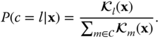
Now, solving the optimization problem of Eq. 8.1, for a given shape ![]() , will provide a segmentation and a labeling of
, will provide a segmentation and a labeling of ![]() . Often, however, we will be dealing with multiple shapes and we would like them to be labeled and segmented in a consistent way. Thus, instead of labeling, say a pair of, 3D models separately from each other, one can do it simultaneously in a process called joint labeling. The goal is to extract parts from the two (or more) input shapes while simultaneously considering their correspondence.
. Often, however, we will be dealing with multiple shapes and we would like them to be labeled and segmented in a consistent way. Thus, instead of labeling, say a pair of, 3D models separately from each other, one can do it simultaneously in a process called joint labeling. The goal is to extract parts from the two (or more) input shapes while simultaneously considering their correspondence.
Let ![]() and
and ![]() be the source and the target shapes. We represent
be the source and the target shapes. We represent ![]() with a graph
with a graph ![]() where the nodes
where the nodes ![]() are surface patches and the edges in
are surface patches and the edges in ![]() connect pairs of adjacent patches. A similar graph
connect pairs of adjacent patches. A similar graph ![]() is also defined for the target shape
is also defined for the target shape ![]() . To perform joint semantic labeling, we define a new graph
. To perform joint semantic labeling, we define a new graph ![]() where
where ![]() and the connectivity
and the connectivity ![]() of the graph is given by two types of arcs, i.e.
of the graph is given by two types of arcs, i.e. ![]() , where
, where
- The intramesh arcs
 are simply given by
  .
. - The intermesh arcs
 connect nodes in
  to nodes in
  based on the similarity of their shape descriptors.
Let also ![]() where
where ![]() is a labeling of
is a labeling of ![]() , and
, and ![]() is a labeling of
is a labeling of ![]() . With this setup, the joint semantic labeling process can be written as the problem of optimizing an energy function of the form:
. With this setup, the joint semantic labeling process can be written as the problem of optimizing an energy function of the form:

The first two terms are the same as the data term and the smoothness term of Eq. 8.1. The third term is the intermesh term. It quantifies how likely it is that two nodes across the two meshes have a specific pair of labels, according to a pairwise cost.
Table 8.1 Potential functions used in the literature for semantic labeling.
| References | Data term |
Smoothness term |
| Kalogerakis et al. 209 |  |
|
| van Kaick et al. 203 | ||
| with |
||
| Sidi et al. 210 | ||
| with |
![]() is the label compatibility term,
is the label compatibility term, ![]() is the dihedral angle between the nodes
is the dihedral angle between the nodes ![]() and
and ![]() ,
, ![]() is the distance between
is the distance between ![]() and
and ![]() ,
, ![]() is the area of the surface patch corresponding to the
is the area of the surface patch corresponding to the ![]() th node, and
th node, and ![]() , and
, and ![]() are some constants.
are some constants.
Implementing the labeling models of Eqs. 8.1 and 8.2 requires:
- Constructing the graph
 and characterizing, using some unary and binary descriptors, the geometry of each of (i) its nodes, which represent the surface patches, and (ii) its edges, which represent the spatial relations between adjacent patches (Section 8.3).
 - Defining the terms of the energy functions and setting their parameters (Section 8.4).
- Solving the optimization problem using some numerical algorithms (Section 8.5).
The subsequent sections describe these aspects in detail. In what follows, we consider that the input shapes have been normalized for translation and scale using any of the normalization methods described in Chapter 2.
8.3 Graph Representation
There are several ways of constructing the intramesh graph ![]() for a given input shape
for a given input shape ![]() . The simplest way is to treat each face of
. The simplest way is to treat each face of ![]() as a node. Two nodes will be connected with an edge if their corresponding faces on
as a node. Two nodes will be connected with an edge if their corresponding faces on ![]() are adjacent. When dealing with large meshes, this method produces large graphs and thus the subsequent steps of the analysis will be computationally very expensive. Another solution is to follow the same concept as superpixels for image analysis 211. For instance, one can decompose a 3D shape into patches. Each patch will be represented with a node in
are adjacent. When dealing with large meshes, this method produces large graphs and thus the subsequent steps of the analysis will be computationally very expensive. Another solution is to follow the same concept as superpixels for image analysis 211. For instance, one can decompose a 3D shape into patches. Each patch will be represented with a node in ![]() . Two nodes will be connected with an edge if their corresponding patches are spatially adjacent on
. Two nodes will be connected with an edge if their corresponding patches are spatially adjacent on ![]() . Figure 8.2 shows an example of a 3D object decomposed into disjoint patches.
. Figure 8.2 shows an example of a 3D object decomposed into disjoint patches.
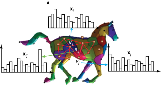
Figure 8.2An example of a surface represented as a graph of nodes and edges. First, the surface is decomposed into patches. Each patch is represented with a node. Adjacent patches are connected with an edge. The geometry of each node  is represented with a unary descriptor
  . The geometric relation between two adjacent nodes
  and
and  is represented with a binary descriptor
  .
.
When jointly labeling a pair of 3D models ![]() and
and ![]() , one can incorporate additional intermesh edges to link nodes in the graph of
, one can incorporate additional intermesh edges to link nodes in the graph of ![]() to nodes in the graph of
to nodes in the graph of ![]() . This will require pairing, or putting in correspondence, patches across
. This will require pairing, or putting in correspondence, patches across ![]() and
and ![]() .
.
8.3.1 Characterizing the Local Geometry and the Spatial Relations
The next step is to compute a set of unary descriptors ![]() , which characterize the local geometry of the graph nodes
, which characterize the local geometry of the graph nodes ![]() , and a set of pairwise descriptors
, and a set of pairwise descriptors ![]() that characterize the spatial relation between adjacent nodes
that characterize the spatial relation between adjacent nodes ![]() and
and ![]() .
.
8.3.1.1 Unary Descriptors
The descriptors ![]() at each node
at each node ![]() characterize the local geometry of the patch represented by
characterize the local geometry of the patch represented by ![]() . They provide cues for patch labeling. In principle, one can use any of the local descriptors described in Chapter 5. Examples include:
. They provide cues for patch labeling. In principle, one can use any of the local descriptors described in Chapter 5. Examples include:
- The shape diameter function (SDF) 212, which gives an estimate of the thickness of the shape at the center of the patch.
- The area of the patch normalized by the total shape area.
- The overall geometry of the patch, which is defined as:
where

 are the three eigenvalues obtained when applying principal component analysis to all the points on the surface of the patch.
Other descriptors that can be incorporated include the principal curvatures within the patch, the average of the geodesic distances 213, the shape contexts 135, and the spin images 95.
8.3.1.2 Binary Descriptors
In addition to the unary descriptors, one can define for each pair of adjacent patches ![]() and
and ![]() , a vector of pairwise features
, a vector of pairwise features ![]() , that provides cues to whether adjacent nodes should have the same label 209. This is used to model the fact that two adjacent patches on the surface of a 3D object are likely to have similar labels. Examples of such pairwise features include:
, that provides cues to whether adjacent nodes should have the same label 209. This is used to model the fact that two adjacent patches on the surface of a 3D object are likely to have similar labels. Examples of such pairwise features include:
- The dihedral angles
 , i.e. the angle between the normal vectors of adjacent patches. The normal vectors can be computed at the center of each patch or as the average of the normal vectors of the patch faces.
 - The distance
 between the centers of the patches
  and
and  . This distance can be Euclidean or geodesic.
These pairwise descriptors are computed for each pair of adjacent nodes ![]() and
and ![]() that are connected with an edge
that are connected with an edge ![]() .
.
8.3.2 Cross Mesh Pairing of Patches
The intermesh edges ![]() , which connect a few nodes in
, which connect a few nodes in ![]() to nodes in
to nodes in ![]() , can be obtained in different ways. For instance, they can be manually provided, e.g. in the form of constraints or prior knowledge. They can be also determined by pairing nodes that have similar geometric descriptors. This is, however, prone to errors since a 3D shape may have several parts that are semantically different but geometrically very similar (e.g. the legs and the tail of a quadruple animal). Since the purpose of these intermesh edges is to guide the joint labeling to ensure consistency, only a few reliable intermesh edges is usually sufficient. These can be efficiently computed in a supervised manner if training data are available.
, can be obtained in different ways. For instance, they can be manually provided, e.g. in the form of constraints or prior knowledge. They can be also determined by pairing nodes that have similar geometric descriptors. This is, however, prone to errors since a 3D shape may have several parts that are semantically different but geometrically very similar (e.g. the legs and the tail of a quadruple animal). Since the purpose of these intermesh edges is to guide the joint labeling to ensure consistency, only a few reliable intermesh edges is usually sufficient. These can be efficiently computed in a supervised manner if training data are available.
Let ![]() and
and ![]() be the graphs of two training shapes
be the graphs of two training shapes ![]() and
and ![]() . Let also
. Let also ![]() be a set of matching pairs of nodes
be a set of matching pairs of nodes ![]() , where
, where ![]() and
and ![]() . We assign to each pair of nodes
. We assign to each pair of nodes ![]() in
in ![]() a label 1 if the pairing is correct, i.e. the node
a label 1 if the pairing is correct, i.e. the node ![]() is a true correspondence to the node
is a true correspondence to the node ![]() , and 0 otherwise. The set of nodes in
, and 0 otherwise. The set of nodes in ![]() and their associated labels can then be used as training samples for learning a binary classifier, which takes a pair of nodes and assigns them the label 1 if the pair is a correct correspondence, and the label 0 otherwise. This is a standard binary classification problem, which, in principle, can be solved using any type of supervised learning algorithm, e.g. Support Vector Machines 214 or AdaBoost 215, 216. van Kaick et al. 203, for example, used GentleBoost 215, 216 to learn this classifier. GentleBoost, just like AdaBoost, is an ensemble classifier, which combines the output of weak classifiers to build a strong classifier. Its advantage is the fact that one can use a large set of descriptor types to characterize the geometry of each node. The algorithm learns from the training examples the descriptors that provide the best performance. It also assigns a confidence, or a weight, to each of the selected descriptors.
and their associated labels can then be used as training samples for learning a binary classifier, which takes a pair of nodes and assigns them the label 1 if the pair is a correct correspondence, and the label 0 otherwise. This is a standard binary classification problem, which, in principle, can be solved using any type of supervised learning algorithm, e.g. Support Vector Machines 214 or AdaBoost 215, 216. van Kaick et al. 203, for example, used GentleBoost 215, 216 to learn this classifier. GentleBoost, just like AdaBoost, is an ensemble classifier, which combines the output of weak classifiers to build a strong classifier. Its advantage is the fact that one can use a large set of descriptor types to characterize the geometry of each node. The algorithm learns from the training examples the descriptors that provide the best performance. It also assigns a confidence, or a weight, to each of the selected descriptors.
The main difficulty with a training‐based approach is in building the list of pairs ![]() and their associated labels. Since these are used only during the training stage, one could do it manually. Alternatively, van Kaick et al. 203 suggested an automatic approach, which operates as follows:
and their associated labels. Since these are used only during the training stage, one could do it manually. Alternatively, van Kaick et al. 203 suggested an automatic approach, which operates as follows:
- First, for a given pair of shapes represented with their graphs
 and
and  , collect all their nodes and compute
  types of geometric descriptors on each of their nodes. These can be any of the unary descriptors described in Section 8.3.1.
 - Next, for each node in
 , select the first
  pairwise assignments with the highest similarity and add them to
  . The similarity is given by the inverse of the Euclidean distance between the descriptors of the two nodes.
 - Finally, build a matrix
 of
of  rows and
  columns where each entry
  stores the dissimilarity between the
  th pair of nodes in
  but computed using the
  th descriptor type.
The matrix ![]() will be used as input to the GentleBoost‐based training procedure, which will learn a strong classifier as a linear combination of weak classifiers, each one is based on one descriptor type. The outcome of the training is a classifier that can label a candidate assignment with true or false. At run time, given a pair of query shapes, select candidate pairs of nodes with the same procedure used during the training stage. Then, using the learned classifier, classify each of these pairs into either a valid or invalid intermesh edge. This procedure produces a small, yet reliable, set of intermesh edges.
will be used as input to the GentleBoost‐based training procedure, which will learn a strong classifier as a linear combination of weak classifiers, each one is based on one descriptor type. The outcome of the training is a classifier that can label a candidate assignment with true or false. At run time, given a pair of query shapes, select candidate pairs of nodes with the same procedure used during the training stage. Then, using the learned classifier, classify each of these pairs into either a valid or invalid intermesh edge. This procedure produces a small, yet reliable, set of intermesh edges.
8.4 Energy Functions for Semantic Labeling
The energy to be minimized by the labeling process, i.e. Eqs. 8.1 and 8.2, is composed of two types of terms: the unary (or data) term and the pairwise (or smoothness) term. The data term takes into consideration how likely it is that a given node has a specific label. The smoothness term considers the intramesh (Eq. 8.1) and intermesh (Eq. 8.2) connectivity between nodes. It quantifies, according to a pairwise cost, how likely it is that two neighboring nodes (i.e. two nodes which are connected with an edge) have a specific pair of labels. Below, we discuss these two terms in more detail. We also refer the reader to Table 8.1.
8.4.1 The Data Term
The data term is defined as the negative log likelihood that a node ![]() is part of a segment labeled
is part of a segment labeled ![]() :
:
where ![]() is the area of the surface patch corresponding to the
is the area of the surface patch corresponding to the ![]() th node. This likelihood can be also interpreted as a classifier, which takes as input the feature vector
th node. This likelihood can be also interpreted as a classifier, which takes as input the feature vector ![]() of a node
of a node ![]() , and returns
, and returns ![]() , the probability distribution of labels for that node. This classifier, which provides a probabilistic labeling of the nodes on the query shapes, can be learned either in a supervised or in a nonsupervised manner, see Section 8.5. It provides a good initial labeling since it captures very well the part interiors but not the part boundaries. This initial labeling can be also interpreted as an initial segmentation where the set of nodes with the same label form a segment.
, the probability distribution of labels for that node. This classifier, which provides a probabilistic labeling of the nodes on the query shapes, can be learned either in a supervised or in a nonsupervised manner, see Section 8.5. It provides a good initial labeling since it captures very well the part interiors but not the part boundaries. This initial labeling can be also interpreted as an initial segmentation where the set of nodes with the same label form a segment.
8.4.2 Smoothness Terms
To refine the result of the probabilistic labeling of Eq. 8.3, one can add other terms to the energy function to impose additional constraints and to incorporate some a‐priori knowledge about the desired labeling. The main role of these terms is to improve the quality of the boundaries between the segments and to prevent incompatible segments from being adjacent. Examples of such constraints include:
8.4.2.1 Smoothness Constraints
In general, adjacent nodes in a 3D model are likely to belong to the same segment. Thus, they should be assigned the same label. The smoothness can then have the following form:
Here, ![]() is a positive constant, which can be interpreted as the cost of having two adjacent nodes labeled differently. For instance, two adjacent nodes are likely to have the same label if their dihedral angle is close to zero, i.e. the patches are coplanar. They are likely to have different labels if they are far apart (large
is a positive constant, which can be interpreted as the cost of having two adjacent nodes labeled differently. For instance, two adjacent nodes are likely to have the same label if their dihedral angle is close to zero, i.e. the patches are coplanar. They are likely to have different labels if they are far apart (large ![]() ) or their corresponding dihedral angle is large. Using these observations, Sidi et al. 210 define
) or their corresponding dihedral angle is large. Using these observations, Sidi et al. 210 define ![]() as:
as:
Here, ![]() where
where ![]() is the distance between the centers of the patches
is the distance between the centers of the patches ![]() and
and ![]() , and
, and ![]() , also known as the dihedral angle, is the angle between the normals to the two patches at their centers.
, also known as the dihedral angle, is the angle between the normals to the two patches at their centers.
8.4.2.2 Geometric Compatibility
In addition to the smoothness constraints, one can incorporate a geometry‐dependent term ![]() , which measures the likelihood of there being a difference in the labels between two adjacent nodes as a function of their geometry. For instance, one can penalize boundaries in flat regions and favor boundaries between the nodes that have a high dihedral angle (i.e. concave regions). One can also use it to penalize the boundary length, which will help in preventing jaggy boundaries and in removing small, isolated segments. van Kaick et al. 203 define this term as:
, which measures the likelihood of there being a difference in the labels between two adjacent nodes as a function of their geometry. For instance, one can penalize boundaries in flat regions and favor boundaries between the nodes that have a high dihedral angle (i.e. concave regions). One can also use it to penalize the boundary length, which will help in preventing jaggy boundaries and in removing small, isolated segments. van Kaick et al. 203 define this term as:
where ![]() and
and ![]() are some real weights that control the importance of each of the two geometric properties (i.e.
are some real weights that control the importance of each of the two geometric properties (i.e. ![]() , which is the distance between the centers of the patches
, which is the distance between the centers of the patches ![]() and
and ![]() , and the dihedral angle
, and the dihedral angle ![]() ).
).
Kalogerakis et al. 209 used a more complex term, which is defined as follows;

The first term, ![]() , measures the probability of two adjacent nodes having distinct labels as a function of their pairwise geometric features
, measures the probability of two adjacent nodes having distinct labels as a function of their pairwise geometric features ![]() . These consist of the dihedral angles between the nodes
. These consist of the dihedral angles between the nodes ![]() and
and ![]() , and the differences of the various local features computed at the nodes, e.g. the differences of the surface curvatures and the surface third‐derivatives, the shape diameter differences, and the differences of distances from the medial surface points. The
, and the differences of the various local features computed at the nodes, e.g. the differences of the surface curvatures and the surface third‐derivatives, the shape diameter differences, and the differences of distances from the medial surface points. The ![]() term of Eq. 8.7 penalizes boundaries between the faces with a high exterior dihedral angle
term of Eq. 8.7 penalizes boundaries between the faces with a high exterior dihedral angle ![]() , following Shapira et al. 217.
, following Shapira et al. 217. ![]() and
and ![]() are small constants, which are set to
are small constants, which are set to ![]() . They are added to avoid computing
. They are added to avoid computing ![]() and to avoid numerical instabilities 217, 218.
and to avoid numerical instabilities 217, 218.
Note that there are similarities between Eqs. 8.6 and 8.7. For instance, the second term of both equations is defined in terms of the dihedral angle ![]() . For the first term, although in both equations it is defined using the distance
. For the first term, although in both equations it is defined using the distance ![]() , Eq. 8.7 uses, in addition to the dihedral angle, more pairwise features and is defined as the log probability of two adjacent nodes having different labels given their pairwise geometric features. It is more general since any type of probability can be used. However, these probabilities should be learned, in a supervised manner, from training data. This will be discussed in Section 8.5.
, Eq. 8.7 uses, in addition to the dihedral angle, more pairwise features and is defined as the log probability of two adjacent nodes having different labels given their pairwise geometric features. It is more general since any type of probability can be used. However, these probabilities should be learned, in a supervised manner, from training data. This will be discussed in Section 8.5.
8.4.2.3 Label Compatibility
Finally, one can impose penalties to some combinations of labeling. For instance, when labeling human body shapes, one can never find two adjacent nodes that are labeled head and torso, respectively. This label‐compatibility constraint can be represented as an ![]() symmetric matrix
symmetric matrix ![]() of penalties for each possible pair of labels (
of penalties for each possible pair of labels (![]() here is the number of possible semantic labels). Note that,
here is the number of possible semantic labels). Note that, ![]() for all
for all ![]() since there is no penalty when there is no discontinuity. The entries of the matrix
since there is no penalty when there is no discontinuity. The entries of the matrix ![]() can be either manually specified or learned in a supervised manner from training data, see Section 8.5.
can be either manually specified or learned in a supervised manner from training data, see Section 8.5.
8.4.3 The Intermesh Term
Finally, the intermesh term ![]() is given by
is given by
where ![]() is a node on the graph of the source mesh,
is a node on the graph of the source mesh, ![]() is a node on the graph of the target mesh, and
is a node on the graph of the target mesh, and ![]() is the label compatibility defined in Section 8.4.2.
is the label compatibility defined in Section 8.4.2. ![]() is the confidence that the assignment between nodes
is the confidence that the assignment between nodes ![]() and
and ![]() is correct. It is computed using the procedure described in Section 8.3.2. The higher the confidence value attached to the assignment is, the more the cost is increased if the labels are different. The parameter
is correct. It is computed using the procedure described in Section 8.3.2. The higher the confidence value attached to the assignment is, the more the cost is increased if the labels are different. The parameter ![]() regulates the influence of the intermesh term to the total energy.
regulates the influence of the intermesh term to the total energy.
8.5 Semantic Labeling
Before we discuss the algorithms that can be used to optimize the energy function of Eqs. 8.1 and 8.2, we will first discuss how to set the different terms. In particular, both the data and smoothness terms of the labeling energy require the probability that a node ![]() is part of a segment labeled
is part of a segment labeled ![]() (Eq. 8.3), and the probability that two adjacent nodes have distinct labels (Eq. 8.7). These two distributions can be learned if some training data is available.
(Eq. 8.3), and the probability that two adjacent nodes have distinct labels (Eq. 8.7). These two distributions can be learned if some training data is available.
Let us assume that for each semantic label ![]() we have
we have ![]() training nodes coming from different models. By computing the descriptors of each node, we obtain a collection of descriptors,
training nodes coming from different models. By computing the descriptors of each node, we obtain a collection of descriptors, ![]() , for each label
, for each label ![]() . These training nodes can be obtained either manually, by labeling some training samples, or automatically, in a nonsupervised manner, by using some unsupervised clustering techniques. We will first look at the latter case, i.e. how to build the training data (i.e. a set of nodes and their corresponding labels) using unsupervised clustering. We will then detail how the probability distributions of Eqs. 8.3 and 8.7 are learned independently of how the training data are obtained.
. These training nodes can be obtained either manually, by labeling some training samples, or automatically, in a nonsupervised manner, by using some unsupervised clustering techniques. We will first look at the latter case, i.e. how to build the training data (i.e. a set of nodes and their corresponding labels) using unsupervised clustering. We will then detail how the probability distributions of Eqs. 8.3 and 8.7 are learned independently of how the training data are obtained.
8.5.1 Unsupervised Clustering
One approach to automatically generate training samples for learning the conditional probability of Eq. 8.3 is by unsupervised clustering in the descriptor space. Let us start with a collection of 3D shapes, each shape is represented with their graphs of nodes. The first step is to pre‐segment, in a nonsupervised manner, each shape by clustering its nodes based on their distance in the descriptor space. Second, all the segments of all the shapes are put together into a single bag. They are then clustered into groups of segments based on their geometric similarities. Each cluster obtained with this procedure corresponds to one semantic component (e.g. legs, handles, etc.) for which we assign a semantic label. Finally, since each cluster contains multiple instances of the semantic class with rich geometric variability, one can learn the statistics of that class. In particular, one can learn ![]() . This process is summarized in Figure 8.3. Below, we describe in detail each of these steps.
. This process is summarized in Figure 8.3. Below, we describe in detail each of these steps.
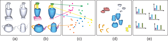
Figure 8.3Unsupervised learning of the statistics of the semantic labels. (a) Training set. (b) Presegmentation of individual shapes. (c) Embedding in the descriptor space. (d) Clustering. (e) Statistical model per semantic label.
- Step 1 – Presegmentation of individual shapes. After computing a shape descriptor
 for each node
  of a given 3D model, one can obtain an initial segmentation of the input 3D shape by clustering in the descriptor space all the nodes of the 3D shape using unsupervised algorithms such as k‐means or mean‐shift 219. Both algorithms require the specification of one parameter; k‐means requires setting in advance the number of clusters. Mean‐shift, on the other hand, operates by finding the modes (i.e. the local maxima of the density or the cluster centers) of points in the descriptor space. The advantage of using mean‐shift lies in that the number of clusters does not have to be known in advance. Instead, the algorithm requires an estimation of the bandwidth or the radius of support around the neighborhood of a point. This can be estimated from the data. For instance, Shamir et al. 220 and Sidi et al. 210 fix the bandwidth to a percentage of the range of each descriptor.
This procedure produces a pre‐segmentation of each individual shape into a set of clusters. The last step is to break spatially disconnected clusters into separate segments.
- Step 2 – Cosegmentation. Next, to produce the final semantic clusters, which will be used to learn the probability distribution of each semantic label, we cluster, in an unsupervised manner, all the segments produced in Step 1. These segments are first embedded into a common space via diffusion map. The embedding translates the similarity between segments into spatial proximity so that a clustering method based on the Euclidean distance will be able to find meaningful clusters in this space.
Let
 be the set of segments obtained for all shapes and let
  be the dissimilarity between two segments
  and
and  . First, we construct an affinity matrix
  such that each of its entries
  is given as:(8.9)
The parameter
 can be compute either manually or automatically from the data by taking the standard deviation of all possible pairwise distances
  .
.Now, let
 be a diagonal matrix such that
  and
and  for
for  . We define the matrix
  , which can be seen as a stochastic matrix with
  being the probability of a transition from the segment
  to the segment
  in one time step. The transition probability can be interpreted as the strength of the connection between the two segments.
Next, we compute the eigendecomposition of the matrix
 and obtain the eigenvalues
  and their corresponding eigenvectors
  . The diffusion map at time
  is given by:(8.10)
Here,
 refers to the
  ‐th entry of the eigenvector
  , and
, and  refers to
  power
power  (Sidi et al. 210 used
  ). The point
  defines the coordinates of the segment
  in the embedding space. In practice, one does not need to use all the eigenvectors. The first leading ones (e.g. the first three) are often sufficient. Note that the eigenvector
  is constant and is thus discarded.
Finally, a cosegmentation is obtained by clustering the segments in the embedded space. Here, basically, any clustering method, e.g. k‐means or fuzzy clustering, can be used. However, the number of clusters, which corresponds to the number of semantic parts (e.g. base, body, handle, or neck of a vase) that constitute the shapes, is usually manually specified by the user.
The output of this procedure is a set of node clusters where each cluster corresponds to one semantic category (e.g. base, body, handle, or neck of a vase) to which we assign a label ![]() .
.
8.5.2 Learning the Labeling Likelihood
The next step is to learn a statistical model of each semantic cluster. For each semantic cluster labeled ![]() , we collect into a set
, we collect into a set ![]() the descriptor values for all of the nodes (surface patches) which form the cluster. One can then learn a conditional probability function
the descriptor values for all of the nodes (surface patches) which form the cluster. One can then learn a conditional probability function ![]() using the descriptors in
using the descriptors in ![]() as positive examples and the remaining descriptors (i.e. the descriptors of the nodes whose labels are different from
as positive examples and the remaining descriptors (i.e. the descriptors of the nodes whose labels are different from ![]() ) as negative ones. This conditional probability defines the likelihood of assigning a certain label for an observed vector of descriptors.
) as negative ones. This conditional probability defines the likelihood of assigning a certain label for an observed vector of descriptors.
To learn this conditional probability distribution, van Kaick et al. 203 first use GentleBoost algorithm 215, 216 to train one classifier per semantic label. Each classifier returns the confidence value ![]() , i.e. the confidence of
, i.e. the confidence of ![]() belonging to the class whose label is
belonging to the class whose label is ![]() . These unnormalized confidence values returned by each classifier are then transformed into probabilities with the softmax activation function as follows:
. These unnormalized confidence values returned by each classifier are then transformed into probabilities with the softmax activation function as follows:
For a given 3D shape, which is unseen during the training phase, this statistical model is used to estimate the probability that each of its nodes ![]() belongs to each of the classes in
belongs to each of the classes in ![]() .
.
8.5.2.1 GentleBoost Classifier
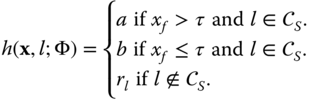
Here, we briefly summarize the GentleBoost classifier and refer the reader to 216 for more details. GentleBoost takes an input feature ![]() and outputs a probability
and outputs a probability ![]() for each possible label
for each possible label ![]() is
is ![]() . It is composed of decision stumps. A decision stump of parameters
. It is composed of decision stumps. A decision stump of parameters ![]() is a very simple classifier that returns a score
is a very simple classifier that returns a score ![]() of each possible class label
of each possible class label ![]() , given a feature vector
, given a feature vector ![]() , based only on thresholding its
, based only on thresholding its ![]() th entry
th entry ![]() . It proceeds as follows:
. It proceeds as follows:
- First, a decision stump stores a set of classes
 .
. - If
 , then the stump compares
  against a threshold
  , and returns a constant
  if
if  , and another constant
  otherwise.
 - If
 , then a constant
  is returned. There is one
  for each
  .
.
This can be written mathematically as follows;
The parameters ![]() of a single decision stump are
of a single decision stump are ![]() ,
, ![]() (the entry of
(the entry of ![]() which is thresholded), the set
which is thresholded), the set ![]() , and
, and ![]() for each
for each ![]() . The probability of a given class
. The probability of a given class ![]() is computed by summing the decision stumps:
is computed by summing the decision stumps:

where ![]() is the
is the ![]() th decision stump and
th decision stump and ![]() are its parameters. The unnormalized confidence value returned by the classifier
are its parameters. The unnormalized confidence value returned by the classifier ![]() for a given feature vector
for a given feature vector ![]() is then given by:
is then given by:
Finally, the probability of ![]() belonging to the class of label
belonging to the class of label ![]() is computed using the softmax transformation of Eq. 8.11.
is computed using the softmax transformation of Eq. 8.11.
8.5.2.2 Training GentleBoost Classifiers
The goal is to learn, from training data, the appropriate number of decision stumps in Eq. 8.13 and the parameters ![]() of each decision stump
of each decision stump ![]() . The input to the training algorithm is a collection of
. The input to the training algorithm is a collection of ![]() pairs
pairs ![]() , where
, where ![]() is a feature vector and
is a feature vector and ![]() is its corresponding label value. Furthermore, each training sample
is its corresponding label value. Furthermore, each training sample ![]() is assigned a per‐class weight
is assigned a per‐class weight ![]() . These depend on whether we are learning the unary term of Eq. 8.3 or the elements of the binary term of Eq. 8.7;
. These depend on whether we are learning the unary term of Eq. 8.3 or the elements of the binary term of Eq. 8.7;
- For the unary term of Eq. 8.3, the training pairs are the per‐node feature vectors and their labels, i.e.
 , for all the graph nodes in the training set. The weight
  is set to be the area of the
  th node.
 - For the pairwise term of Eq. 8.7, the training pairs are the pairwise feature vectors (see Section 8.3.1) and their binary labels. That is
 . The weight
  is used to reweight the boundary edges, since the training data contain many more nonboundary edges. Let
  and
and  be, respectively, the number of boundary edges and the number of nonboundary edges. Then,
  for boundary edges and
  for nonboundary edges, where
  is the corresponding edge length.
GentleBoost learns the appropriate number of decisions stumps and the parameters of each decision stump which minimize the weighted multiclass exponential loss over the training set:
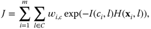
where ![]() is given by Eq. 8.13, and
is given by Eq. 8.13, and ![]() is an indicator function. It takes the value of 1 when
is an indicator function. It takes the value of 1 when ![]() and the value
and the value ![]() otherwise. The training is performed iteratively as follows:
otherwise. The training is performed iteratively as follows:
- Set
 .
. - At each iteration, add one decision stump (Eq. 8.12) to the classifier.
- Compute the parameters
 of the newly added decision stump
  by optimizing the following weighted least‐squares objective:
(8.16)
by optimizing the following weighted least‐squares objective:
(8.16)
- Update the weights
 as follows;
(8.17)
as follows;
(8.17)
- Repeat from Step 2. The algorithms stops after a few hundred iterations.
Following Torralba et al. 216, the optimal ![]() are computed in closed‐form, and
are computed in closed‐form, and ![]() are computed by brute‐force. When the number of labels is greater than 6, the greedy heuristic search is used for
are computed by brute‐force. When the number of labels is greater than 6, the greedy heuristic search is used for ![]() .
.
Belonging to the family of boosting algorithms, GentleBoost has many appealing properties: it performs automatic feature selection and can handle large numbers of input features for multiclass classification. It has a fast learning algorithm. It is designed to share features among classes, which greatly reduces the generalization error for multiclass recognition when classes overlap in the feature space.
8.5.3 Learning the Remaining Parameters
The remaining parameters, ![]() (Eqs. 8.6 and 8.7),
(Eqs. 8.6 and 8.7), ![]() (the label compatibility, see the second row of Table 8.1), and
(the label compatibility, see the second row of Table 8.1), and ![]() (Eq. 8.8), can be learned by performing a grid search over a specified range. Given a training dataset, and for each possible value of these parameters, one can evaluate the classification accuracy and select those which give the best score. One possible measure of the classification accuracy is the Segment‐Weighted Error of Kalogerakis et al. 209, which weighs each segment equally:
(Eq. 8.8), can be learned by performing a grid search over a specified range. Given a training dataset, and for each possible value of these parameters, one can evaluate the classification accuracy and select those which give the best score. One possible measure of the classification accuracy is the Segment‐Weighted Error of Kalogerakis et al. 209, which weighs each segment equally:
where ![]() is the area of the
is the area of the ![]() th node,
th node, ![]() is the ground‐truth label for the
is the ground‐truth label for the ![]() th node,
th node, ![]() is the output of the classifier for the
is the output of the classifier for the ![]() th node,
th node, ![]() is the total area of all nodes (patches) within the segment
is the total area of all nodes (patches) within the segment ![]() that has ground‐truth label
that has ground‐truth label ![]() , and
, and ![]() if
if ![]() , and zero otherwise.
, and zero otherwise.
To improve the computation efficiency, these parameters can be optimized in two steps. First, the error is minimized over a coarse grid in the parameter space by brute‐force search. Second, starting from the minimal point in the grid, the optimization continues using the MATLAB implementation of Preconditioned Conjugate Gradient with numerically‐estimated gradients 209.
8.5.4 Optimization Using Graph Cuts
Now that we have defined all the ingredients, the last step is to solve the optimizations of Eqs. 8.1 and 8.2. One can use for this purpose multilabel graph‐cuts to assign labels to the nodes in an optimal manner. In general, graph‐cuts algorithms require the pairwise term to be a metric. This is not necessarily the case in our setup. Thus, one can use the ![]() swap algorithm 221. By minimizing the given energy, we obtain the most likely label for each graph node (and thus surface patch) while also avoiding the creation of small disconnected segments. Algorithm 8.1 summarizes the graph cut's
swap algorithm 221. By minimizing the given energy, we obtain the most likely label for each graph node (and thus surface patch) while also avoiding the creation of small disconnected segments. Algorithm 8.1 summarizes the graph cut's ![]() swap algorithm. We refer the reader to the paper of Boykov et al. 221 for a detailed discussion of the algorithm.
swap algorithm. We refer the reader to the paper of Boykov et al. 221 for a detailed discussion of the algorithm.

8.6 Examples
In this section, we show a few semantic labeling and correspondence examples obtained using the techniques discussed in this chapter. In particular, we will discuss the importance of each of the energy terms of Eqs. 8.1 and 8.2.
First, Figure 8.4 shows that ![]() , and subsequently the data term of Eqs. 8.1 and 8.2, captures the main semantic regions of a 3D shape but fails to accurately capture the boundaries of the semantic regions. By adding the intramesh term, the boundaries become smoother and well localized (Figure 8.5).
, and subsequently the data term of Eqs. 8.1 and 8.2, captures the main semantic regions of a 3D shape but fails to accurately capture the boundaries of the semantic regions. By adding the intramesh term, the boundaries become smoother and well localized (Figure 8.5).

Figure 8.4Effects of the unary term  on the quality of the segmentation.
Source: The image has been adapted from the powerpoint presentation of Kalogerakis et al. 209 with the permission of the author.
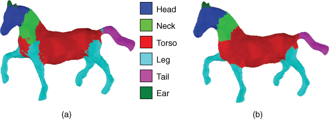
Figure 8.5Semantic labeling by using (a) only the unary term of Eq. 8.1 and (b) the unary and binary terms of Eq. 8.1. The result in (b) is obtained using the approach of Kalogerakis et al. 209, i.e. using the unary term and binary term defined in the first row of Table 8.1.
Source: The image has been adapted from the powerpoint presentation of Kalogerakis et al. 209 with the permission of the author.
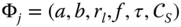
Figure 8.6 shows samples from the training datasets, which were used as prior knowledge for learning the labeling. Note that, although at runtime the shapes are processed individually, the approach is able to label multiple shapes in a consistent manner. Thus, the labeling provides simultaneously a semantic segmentation and also partwise correspondences between the 3D models. Figure 8.6 also shows the effect of the training data on the labeling. In fact, different segmentation and labeling results are obtained when using different training datasets.

Figure 8.6Supervised labeling using the approach of Kalogerakis et al. 209. Observe that different training sets lead to different labeling results. The bottom row image is from Reference 209.
©2010 ACM, Inc. Reprinted by permission. http://doi.acm.org/10.1145/1778765.1778839
Finally, Figure 8.7 demonstrates the importance of the intermesh term, and subsequently the joint labeling process. In Figure 8.7a, the correspondence is computed based purely on the prior knowledge, i.e. by only using the unary and intramesh terms of Eq. 8.1. Observe that part of the support of the candle on the right is mistakenly labeled as a handle and, therefore, does not have a corresponding part on the shape on the left. However, when the intramesh term (i.e. Eq. 8.2), is taken into consideration, we obtain a more accurate correspondence, as shown in Figure 8.7b, since the descriptors of the thin structures on both shapes are similar. We observe an analogous situation in the chairs, where the seat of the chair is mistakenly labeled as a backrest, due to the geometric distortion present in the model. In Figure 8.7b, the joint labeling is able to obtain the correct part correspondence, guided by the similarity of the seats. This demonstrates that both knowledge and content are essential for finding the correct correspondence in these cases.

Figure 8.7Effect of the intermesh term on the quality of the semantic labeling. Results are obtained using the approach of van Kaick et al. 203, i.e. using the energy functions of the second row of Table 8.1. (a) Semantic labeling without the intermesh term (i.e. using the energy of Eq. 8.1). (b) Semantic labeling using the intermesh term (i.e. using the energy of Eq. 8.2).
Source: The image has been adapted from 203.
8.7 Summary and Further Reading
We have presented in this chapter some mathematical tools for computing correspondences between 3D shapes that differ in geometry and topology but share some semantic similarities. The set of solutions, which we covered in this chapter, treat this problem as a joint semantic labeling process, i.e. simultaneously and consistently labeling the regions of two or more surfaces. This is formulated as a problem of minimizing an energy function composed of multiple terms; a data term, which encodes the a‐priori knowledge about the semantic labels, and one or more terms, which constrain the solution. Most of existing techniques differ in the type of constraints that are encoded in these terms and the way the energy function is optimized.
The techniques presented in this chapter are based on the work of (i) Kalogerakis et al. 209, which presented a data‐driven approach to simultaneous segmentation and labeling of parts in 3D meshes, (ii) van Kaick et al. 203, which used prior knowledge to learn semantic correspondences, and (iii) Sidi et al. 210, which presented a unsupervised method for jointly segmenting and putting in correspondence multiple objects belonging to the same family of 3D shapes. These are just examples of the state‐of‐the‐art. Other examples include the work of Huang et al. 222, which used linear programming for joint segmentation and labeling, and Laga et al. 204, 223, which observed that structure, i.e. the way shape components are interconnected to each other, can tell a lot about the semantic of a shape. They designed a metric that captures structural similarities. The metric is also used for partwise semantic correspondence and for functionality recognition in man‐made 3D shapes. Feragen et al. 224 considered 3D shapes that have a tree‐like structure and developed a framework, which enables computing correspondences and geodesics between such shapes. The framework has been applied to the analysis of airways trees 224 and botanical trees 225.
Finally, semantic analysis of 3D shapes has been extensively used for efficient modeling and editing of 3D shapes 226–228 and for exploring 3D shape collections 229. For further reading, we refer the reader to the surveys of Mitra et al. 205 on structure‐aware shape processing and to the survey of van Kaick et al. 183 on 3D shape correspondence.