2
Basic Elements of 3D Geometry and Topology
This chapter introduces some of the fundamental concepts of 3D geometry and 3D geometry processing. Since this is a very large topic, we only focus in this chapter on the concepts that are relevant to the 3D shape analysis tasks covered in the subsequent chapters. We structure this chapter into two main parts. The first part (Section 2.1) covers the elements of differential geometry that are used to describe the local properties of 3D shapes. The second part (Section 2.2) defines the concept of shape, the transformations that preserve the shape of a 3D object, and the deformations that affect the shape of 3D objects. It also describes some preprocessing algorithms, e.g. alignment, which are used to prepare 3D models for shape analysis tasks.
2.1 Elements of Differential Geometry
2.1.1 Parametric Curves
A one‐dimensional curve in ![]() can be represented in a parametric form by a vector‐valued function of the form:
can be represented in a parametric form by a vector‐valued function of the form:

The functions ![]() , and
, and ![]() are also called the coordinate functions. If we assume that they are differentiable functions of
are also called the coordinate functions. If we assume that they are differentiable functions of ![]() , then one can compute the tangent vector, the normal vector, and the curvature at each point on the curve. For instance, the tangent vector,
, then one can compute the tangent vector, the normal vector, and the curvature at each point on the curve. For instance, the tangent vector, ![]() , to the curve at a point
, to the curve at a point ![]() , see Figure 2.1, is the first derivative of the coordinate functions:
, see Figure 2.1, is the first derivative of the coordinate functions:
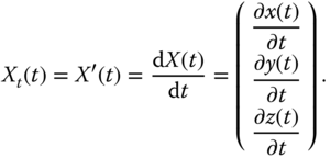
Note that the tangent vector ![]() also corresponds to the velocity vector at time
also corresponds to the velocity vector at time ![]() .
.
Now, let ![]() . The length
. The length ![]() of the curve segment defined between the two points
of the curve segment defined between the two points ![]() and
and ![]() is given by the integral of the tangent vector:
is given by the integral of the tangent vector:

Here, ![]() denotes the inner dot product. The length
denotes the inner dot product. The length ![]() of the curve is then given by
of the curve is then given by ![]() .
.
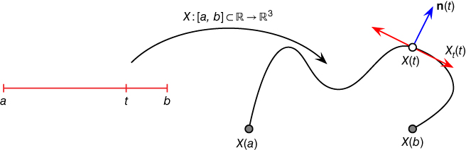
Figure 2.1An example of a parameterized curve and its differential properties.
Let ![]() be a smooth and monotonically increasing function, which maps the domain
be a smooth and monotonically increasing function, which maps the domain ![]() onto
onto ![]() such that
such that ![]() . Reparameterizing
. Reparameterizing ![]() with
with ![]() results in another curve
results in another curve ![]() such that:
such that:
The length of the curve from ![]() to
to ![]() , is exactly
, is exactly ![]() . The mapping function
. The mapping function ![]() , as defined above, is called arc‐length parameterization. In general,
, as defined above, is called arc‐length parameterization. In general, ![]() can be any arbitrary smooth and monotonically increasing function, which maps the domain
can be any arbitrary smooth and monotonically increasing function, which maps the domain ![]() into another domain
into another domain ![]() . If
. If ![]() is a bijection and its inverse
is a bijection and its inverse ![]() is differentiable as well, then
is differentiable as well, then ![]() is called a diffeomorphism. Diffeomorphisms are very important in shape analysis. For instance, as shown in Figure 2.2, reparameterizing a curve
is called a diffeomorphism. Diffeomorphisms are very important in shape analysis. For instance, as shown in Figure 2.2, reparameterizing a curve ![]() with a diffeomorphism
with a diffeomorphism ![]() results in another curve
results in another curve ![]() , which has the same shape as
, which has the same shape as ![]() . These two curves are, therefore, equivalent from the shape analysis perspective.
. These two curves are, therefore, equivalent from the shape analysis perspective.

Figure 2.2Reparameterizing a curve  with a diffeomorphism
  results in another curve
  of the same shape as
  . (a) A parametric curve
  . (b) A reparameterization function
  . (c) The reparametrized curve
  .
.
Now, for simplicity, we assume that ![]() is a curve parameterized with respect to its arc length. We can define the curvature at a point
is a curve parameterized with respect to its arc length. We can define the curvature at a point ![]() as the deviation of the curve from the straight line. It is given by the norm of the second derivative of the curve:
as the deviation of the curve from the straight line. It is given by the norm of the second derivative of the curve:

Curvatures carry a lot of information about the shape of a curve. For instance, a curve with zero curvature everywhere is a straight line segment, and planar curves of constant curvature are circular arcs.
2.1.2 Continuous Surfaces
We will look in this section at the same concepts as those defined in the previous section for curves but this time for smooth surfaces embedded in ![]() .
.
A parametric surface ![]() (see Figure 2.3) can be defined as a vector‐valued function
(see Figure 2.3) can be defined as a vector‐valued function ![]() which maps a two‐dimensional domain
which maps a two‐dimensional domain ![]() onto
onto ![]() . That is:
. That is:
where ![]() , and
, and ![]() are differentiable functions with respect to
are differentiable functions with respect to ![]() and
and ![]() . The domain
. The domain ![]() is called the parameter space, or parameterization domain, and the scalars
is called the parameter space, or parameterization domain, and the scalars ![]() are the coordinates in the parameter space.
are the coordinates in the parameter space.

Figure 2.3Example of an open surface parameterized by a 2D domain  .
.
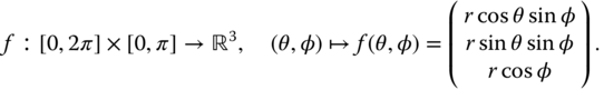
As an example, consider ![]() to be the surface of a sphere of radius
to be the surface of a sphere of radius ![]() and centered at the origin. This surface can be defined using a parametric function of the form
and centered at the origin. This surface can be defined using a parametric function of the form
In practice, the parameter space ![]() is chosen depending on the types of shapes at hand. In the case of open surfaces such as 3D human faces,
is chosen depending on the types of shapes at hand. In the case of open surfaces such as 3D human faces, ![]() can be a subset of
can be a subset of ![]() , e.g. the quadrilateral domain
, e.g. the quadrilateral domain ![]() or the disk domain
or the disk domain ![]() . In the case of closed surfaces, such as those shown in Figure 2.4a,b, then
. In the case of closed surfaces, such as those shown in Figure 2.4a,b, then ![]() can be chosen to be the unit sphere
can be chosen to be the unit sphere ![]() . In this case,
. In this case, ![]() and
and ![]() are the spherical coordinates such that
are the spherical coordinates such that ![]() is the polar angle and
is the polar angle and ![]() is the azimuthal angle.
is the azimuthal angle.
Let ![]() be a diffeomorphism, i.e. a smooth invertible function that maps the domain
be a diffeomorphism, i.e. a smooth invertible function that maps the domain ![]() to itself such that both
to itself such that both ![]() and its inverse are smooth. Let also
and its inverse are smooth. Let also ![]() denote the space of all such diffeomorphisms.
denote the space of all such diffeomorphisms. ![]() transforms a surface
transforms a surface ![]() into
into ![]() . This is a reparameterization process and often
. This is a reparameterization process and often ![]() is referred to as a reparameterization function. Reparameterization is important in 3D shape analysis because it produces registration. For instance, similar to the curve case, both surfaces represented by
is referred to as a reparameterization function. Reparameterization is important in 3D shape analysis because it produces registration. For instance, similar to the curve case, both surfaces represented by ![]() and
and ![]() have the same shape and thus are equivalent. Also, consider the two surfaces
have the same shape and thus are equivalent. Also, consider the two surfaces ![]() and
and ![]() of Figure 2.4b where
of Figure 2.4b where ![]() represents the surface of one long hand and
represents the surface of one long hand and ![]() represents the surface of the hand of another subject. Let
represents the surface of the hand of another subject. Let ![]() be such that
be such that ![]() corresponds to the thumb tip of
corresponds to the thumb tip of ![]() . If
. If ![]() and
and ![]() are arbitrarily parameterized, which is often the case since they have been parameterized independently from each other,
are arbitrarily parameterized, which is often the case since they have been parameterized independently from each other, ![]() may refer to any other location on
may refer to any other location on ![]() , the fingertip of the index finger, for example. Thus,
, the fingertip of the index finger, for example. Thus, ![]() and
and ![]() are not in correct correspondence. Putting
are not in correct correspondence. Putting ![]() and
and ![]() in correspondence is equivalent to reparameterizing
in correspondence is equivalent to reparameterizing ![]() with a diffeomorphism
with a diffeomorphism ![]() such that for every
such that for every ![]() ,
, ![]() and
and ![]() point to the same feature, e.g. thumb tip to thumb tip. We will use these properties in Chapter 7 to find correspondences and register surfaces which undergo complex nonrigid deformations.
point to the same feature, e.g. thumb tip to thumb tip. We will use these properties in Chapter 7 to find correspondences and register surfaces which undergo complex nonrigid deformations.

Figure 2.4Illustration of (a) a spherical parameterization of a closed genus‐0 surface, and (b) how parameterization provides correspondence. Here, the two surfaces, which bend and stretch, are in correct correspondence. In general, however, the analysis process should find the optimal reparameterization which brings  into a full correspondence with
  .
.
2.1.2.1 Differential Properties of Surfaces
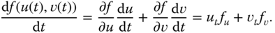
Similar to the curve case, one can define various types of differential properties of a given surface. For instance, the two partial derivatives
define two tangent vectors to the surface at a point of coordinates ![]() . The plane spanned by these two orthogonal vectors is tangent to the surface. The surface unit normal vector at
. The plane spanned by these two orthogonal vectors is tangent to the surface. The surface unit normal vector at ![]() , denoted by
, denoted by ![]() , can be computed as:
, can be computed as:
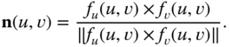
Here, ![]() denotes the vector cross product.
denotes the vector cross product.
First Fundamental Form
A tangent vector ![]() to the surface at a point
to the surface at a point ![]() can be defined in terms of the partial derivatives of
can be defined in terms of the partial derivatives of ![]() as:
as:
The two real‐valued scalars ![]() and
and ![]() can be seen as the coordinates of
can be seen as the coordinates of ![]() in the local coordinate system formed by
in the local coordinate system formed by ![]() and
and ![]() . Let
. Let ![]() and
and ![]() be two tangent vectors of coordinates
be two tangent vectors of coordinates ![]() and
and ![]() , respectively. Then, the inner product
, respectively. Then, the inner product ![]() , where
, where ![]() is the angle between the two vectors, is defined as:
is the angle between the two vectors, is defined as:

where ![]() is a 2D matrix called the first fundamental form of the surface at a point
is a 2D matrix called the first fundamental form of the surface at a point ![]() of coordinates
of coordinates ![]() . Let us write
. Let us write

The first fundamental form, also called the metric or metric tensor, defines inner products on the tangent space to the surface. It allows to measure:
- Angles. The angle between the two tangent vectors
 and
and  can be computed as:

- Length. Consider a curve on the parametric surface. The parametric representation of the curve is
 . The tangent vector to the curve at any point is given as:
Since the curve is on the surface defined by the parametric function
 , then
  and
and  are two orthogonal vectors that are tangent to the surface. Using Eq. (2.3), the length
  of the curve is given by
- Area. Similarly, we can measure the surface area
 of a certain region
  :
:
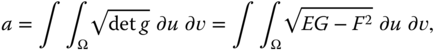
where
 refers to the determinant of the square matrix
  .
.
Since the first fundamental form allows measuring angles, distances, and surface areas, it is a strong geometric tool for 3D shape analysis.
Second Fundamental Form and Shape Operator
The second fundamental form ![]() of a surface, defined by its parametric function
of a surface, defined by its parametric function ![]() , at a point
, at a point ![]() is a
is a ![]() matrix defined in terms of the second derivatives of
matrix defined in terms of the second derivatives of ![]() as follows:
as follows:

where

Here, ![]() refers to the standard inner product in
refers to the standard inner product in ![]() , i.e. the Euclidean space. Similarly, the shape operator
, i.e. the Euclidean space. Similarly, the shape operator ![]() of the surface is defined at a point
of the surface is defined at a point ![]() using the first and second fundamental forms as follows:
using the first and second fundamental forms as follows:
The shape operator is a linear operator. Along with the second fundamental form, they are used for computing surface curvatures.
2.1.2.2 Curvatures
Let ![]() be the unit normal vector to the surface at a point
be the unit normal vector to the surface at a point ![]() , and
, and ![]() a tangent vector to the surface at
a tangent vector to the surface at ![]() . The intersection of the plane spanned by the two vectors
. The intersection of the plane spanned by the two vectors ![]() and
and ![]() with the surface at
with the surface at ![]() forms a curve
forms a curve ![]() called the normal curve. This is illustrated in Figure 2.5. Rotating this plane, which is also called the normal plane, around the normal vector
called the normal curve. This is illustrated in Figure 2.5. Rotating this plane, which is also called the normal plane, around the normal vector ![]() is equivalent to rotating the tangent vector
is equivalent to rotating the tangent vector ![]() around
around ![]() . This will result in a different normal curve. By analyzing the curvature of such curves, we can define the curvature of the surface.
. This will result in a different normal curve. By analyzing the curvature of such curves, we can define the curvature of the surface.
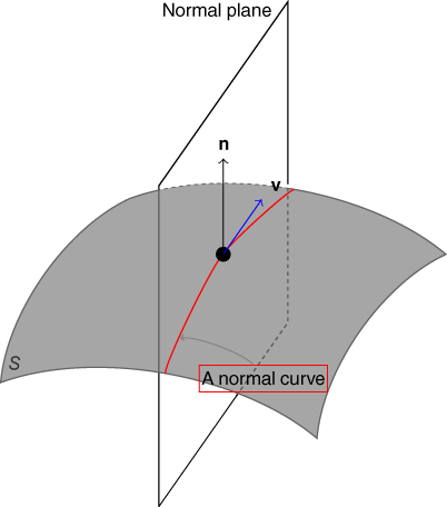
Figure 2.5Illustration of the normal vector, normal plane, and normal curve.
- Normal curvature. The normal curvature
 to the surface at a point
  in the direction of a tangent vector
  is defined as the curvature of the normal curve
  created by intersecting the surface at
  with the plane spanned by
  and
and  . Let
. Let  denote the representation of
  in the 2D local coordinate system spanned by the two orthogonal vectors
  and
and  , i.e.
 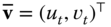 . Then, the normal curvature at
  in the direction of
  can be computed using the first and second fundamental forms as follows:
(2.14)
can be computed using the first and second fundamental forms as follows:
(2.14)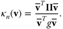
- Principal curvatures. By rotating the tangent vector
 around the normal vector
  , we obtain an infinite number of normal curves at
  . Thus,
  varies with
  . It has, however, two extremal values called principal curvatures; one is the minimum curvature, denoted by
  , and the other is the maximum curvature, denoted by
  .
.
The principal directions,
 and
and  , are the tangent vectors to the normal curves, which have the minimum, respectively the maximum, curvature at
  . These principal directions are orthogonal and thus they form a local orthonormal basis. Consequently, any vector
  that is tangent to the surface at
  can be defined with respect to this basis. For simplicity of notation, let
  and let
  be the angle between
  and
and  . The Euler theorem states that the normal curvature at
  in the direction of
  is given by(2.15)
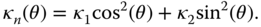
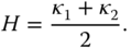
- Mean and Gaussian curvatures. The mean curvature is defined as the average of the two principal curvatures:
(2.16)
The Gaussian curvature, on the other hand, is defined as the product of the two principal curvatures:
(2.17)
These two curvature measures are very important and they are extensively used in 3D shape analysis. For instance, the Gaussian curvature can be used to classify surface points into three distinct categories: elliptical points ![]() , hyperbolic points
, hyperbolic points ![]() , and parabolic points
, and parabolic points ![]() . Figure 2.6 illustrates the relation between different curvatures at a given surface point and the shape of the local patch around that point. For example:
. Figure 2.6 illustrates the relation between different curvatures at a given surface point and the shape of the local patch around that point. For example:
- When the minimum and maximum curvatures are equal and nonzero (i.e. both are either strictly positive or strictly negative) at a given point then the patch around that point is locally spherical.
- When both minimum and maximum curvatures are zero, then the shape is planar.
- When the minimum curvature is zero and the maximum curvature is strictly positive then the shape of the local patch is parabolic. If every point on the surface of a 3D object satisfies this condition and if the maximum curvature is constant everywhere then the 3D object is a cylinder.
- If both curvatures are strictly positive then the shape is elliptical.
- If the minimum curvature is negative while the maximum curvature is positive then the shape is hyperbolic.
Finally, the curvatures can be also defined using the shape operator. For instance, the normal curvature of the surface at a point ![]() in the direction of a tangent vector
in the direction of a tangent vector ![]() is defined as
is defined as
The eigenvalues of ![]() are the principal curvatures at
are the principal curvatures at ![]() . Its determinant is the Gaussian curvature and its trace is twice the mean curvature at
. Its determinant is the Gaussian curvature and its trace is twice the mean curvature at ![]() .
.

Figure 2.6Curvatures provide information about the local shape of a 3D object.
2.1.2.3 Laplace and Laplace–Beltrami Operators
Let ![]() be a function in the Euclidean space. The Laplacian
be a function in the Euclidean space. The Laplacian ![]() of
of ![]() is defined as the divergence of the gradient, i.e.;
is defined as the divergence of the gradient, i.e.;

The Laplace–Beltrami operator is the extension of the Laplace operator to functions defined on manifolds:
where ![]() is a function on the manifold
is a function on the manifold ![]() . If
. If ![]() is a parametric representation of a surface, as defined in Eq. (2.6), then
is a parametric representation of a surface, as defined in Eq. (2.6), then
Here, ![]() and
and ![]() denote, respectively, the Gaussian curvature and the normal vector at a point
denote, respectively, the Gaussian curvature and the normal vector at a point ![]() .
.
2.1.3 Manifolds, Metrics, and Geodesics
The surface of a 3D object can be seen as a domain that is nonlinear, i.e. it is not a vector space. Often, one needs to perform some differential (e.g. computing normals and curvatures) and integral (e.g. tracing curves and paths) calculus on this type of general domains, which are termed manifolds. Below, we provide the necessary definitions.
This definition of topological spaces is the most general notion of a mathematical space, which allows for the definition of concepts such as continuity, connectedness, and convergence. Other spaces are special cases of topological spaces with additional structures or constraints.
Two points ![]() and
and ![]() in a topological space can be separated by neighborhoods if there exists a neighborhood
in a topological space can be separated by neighborhoods if there exists a neighborhood ![]() of
of ![]() and a neighborhood
and a neighborhood ![]() of
of ![]() such that
such that ![]() and
and ![]() are disjoint
are disjoint ![]() . The topological space is a Hausdorff space if all distinct points in it are pairwise neighborhood‐separable.
. The topological space is a Hausdorff space if all distinct points in it are pairwise neighborhood‐separable.
In our applications of geometry, purely topological manifolds are not sufficient. We would like to be able to evaluate first and higher derivatives of functions on our manifold. A differentiable manifold is a manifold with a smoother structure, which allows for the definition of derivatives. Having a notion of differentiability at hand, we can do differential calculus on the manifold and talk about concepts such as tangent vectors, vector fields, and inner products.
If we glue together all the tangent spaces ![]() , we obtain the tangent bundle
, we obtain the tangent bundle ![]() .
.
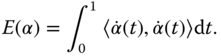
Endowing a manifold with a Riemannian metric makes it possible to define on that manifold geometric notions such as angles, lengths of curves, curvatures, and gradients. With a Riemannian metric, it also becomes possible to define the length of a path on a manifold. Let ![]() be a parameterized path on a Riemannian manifold
be a parameterized path on a Riemannian manifold ![]() , such that
, such that ![]() is differentiable everywhere on
is differentiable everywhere on ![]() . Then,
. Then, ![]() , the velocity vector at
, the velocity vector at ![]() , is an element of the tangent space
, is an element of the tangent space ![]() . Its length is
. Its length is ![]() . The length of the path
. The length of the path ![]() is then given by:
is then given by:
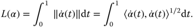
This is the integral of the lengths of the velocity vectors along ![]() and, hence, is the length of the whole path
and, hence, is the length of the whole path ![]() . For any two points
. For any two points ![]() , one can define the distance between them as the infimum of the lengths of all smooth paths on
, one can define the distance between them as the infimum of the lengths of all smooth paths on ![]() that start at
that start at ![]() and end at
and end at ![]() :
:

This definition turns ![]() into a metric space, with distance
into a metric space, with distance ![]() .
.
Very often, the search for geodesics is handled by changing the objective functional from length to an energy functional of the form:
The only difference from the path length in Eq. (2.22) is that the square root in the integrand has been removed. It can be shown that a critical point of this functional restricted to paths between ![]() and
and ![]() is a geodesic between
is a geodesic between ![]() and
and ![]() . Furthermore, of all the reparameterizations of a geodesic, the one with a constant speed has the minimum energy. As a result, for a minimizing path
. Furthermore, of all the reparameterizations of a geodesic, the one with a constant speed has the minimum energy. As a result, for a minimizing path ![]() , we have
, we have
2.1.4 Discrete Surfaces
In the previous section, we treated the surface of a 3D object as a continuous function ![]() . However, most of the applications (including visualization and 3D analysis tasks) require the discretization of these surfaces. Moreover, as will be seen in Chapter , most of 3D acquisition devices and 3D modeling software produce discrete 3D data. For example, scanning devices such as the Kinect and stereo cameras produce depth maps and 3D point clouds. CT scanners in medical imaging produce volumetric images. These are then converted into polygonal meshes, similar to what is produced by most of the 3D modeling software, for rendering and visualization. 3D shape analysis algorithms take as input 3D models in one of these representations and convert them into a representation (a set of features and descriptors), which is suitable for comparison and analysis. Thus, it is important to understand these representations (Section 2.1.4.1) and the data structures used for their storage and processing (Section 2.1.4.2).
. However, most of the applications (including visualization and 3D analysis tasks) require the discretization of these surfaces. Moreover, as will be seen in Chapter , most of 3D acquisition devices and 3D modeling software produce discrete 3D data. For example, scanning devices such as the Kinect and stereo cameras produce depth maps and 3D point clouds. CT scanners in medical imaging produce volumetric images. These are then converted into polygonal meshes, similar to what is produced by most of the 3D modeling software, for rendering and visualization. 3D shape analysis algorithms take as input 3D models in one of these representations and convert them into a representation (a set of features and descriptors), which is suitable for comparison and analysis. Thus, it is important to understand these representations (Section 2.1.4.1) and the data structures used for their storage and processing (Section 2.1.4.2).
2.1.4.1 Representations of Discrete Surfaces
Often, complex surfaces cannot be represented with a single parametric function. In that case, one can use a piecewise representation. For instance, one can partition a complex surface into smaller subregions, called patches, and approximate each patch with one parametric function. The main mathematical challenge here is to ensure continuity between adjacent patches. The most common piecewise representations are spline surfaces, polygonal meshes, and point sets. The spline representation is the standard representation in modern computer aided design (CAD) models. It is used to construct high‐quality surfaces and for surface deformation tasks. In this chapter, we will focus on the second and third representations since they are the most commonly used representations for 3D shape analysis. We, however, refer the reader to other textbooks, such as 1, for a detailed description of spline representations.

Figure 2.7Representations of complex 3D objects: (a) triangular mesh‐based representation and (b) depth map‐based representation.
(1) Polygonal meshes. In a polygonal representation, a 3D model is defined as a collection, or union, of planar polygons. Each planar polygon, which approximates a surface patch, is represented with a set of vertices and a set of edges connecting these vertices. In principle, these polygons can be of arbitrary type. In fact, they are not even required to be planar. In practice, however, triangles are the most commonly used since they are guaranteed to be piecewise linear. In other words, triangles are the only polygons that are always guaranteed to be planar. A surface approximated with a set of triangles is referred to as a triangular mesh. It consists of a set of vertices
and a set of triangular faces
connecting them, see Figure 2.7a. This representation can be also interpreted as a graph ![]() whose nodes are the vertices of the mesh. Its edges
whose nodes are the vertices of the mesh. Its edges ![]() are the edges of the triangular faces. In this graph representation, each triangular face defines, using the barycentric coordinates, a linear parameterization of its interior points. That is, every point
are the edges of the triangular faces. In this graph representation, each triangular face defines, using the barycentric coordinates, a linear parameterization of its interior points. That is, every point ![]() in the interior of a triangle
in the interior of a triangle ![]() can be written as
can be written as ![]() where
where ![]() , and
, and ![]() and
and ![]() .
.
Obviously, the accuracy of the representation depends on the number of vertices (and subsequently the number of faces) that are used to approximate the surface. For instance, a nearly planar surface can be accurately represented using only a few vertices and faces. Surfaces with complex geometry, however, require a large number of faces especially at regions of high curvature.
A singular, or nonmanifold, vertex is a vertex that is attached to two fans of triangles as shown in Figure 2.8a,b. A singular, or nonmanifold, edge is an edge that is attached to more than two faces, see Figure 2.8c. Manifold surfaces are often referred to as watertight models.
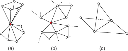
Figure 2.8Examples of nonmanifold surfaces. (a) A nonmanifold vertex attached two fans of triangles, (b) a nonmanifold vertex attached to patches, and (c) a nonmanifold edge attached to three faces.
Manifoldness is an important property of triangular meshes. In particular, a manifold surface ![]() can always be locally parameterized at each point
can always be locally parameterized at each point ![]() using a function
using a function ![]() , where
, where ![]() is a planar domain, e.g. a disk or a square. As such, differential properties (see Section 2.1.2) can efficiently be computed using some analytical approximations.
is a planar domain, e.g. a disk or a square. As such, differential properties (see Section 2.1.2) can efficiently be computed using some analytical approximations.
When the mesh is nonmanifold, it is often referred to as a polygon soup model. Polygon soup models are easier to create since one does not have to worry about the connectivity of the vertices and edges. They are, however, problematic for some shape analysis algorithms since the differential properties of such surfaces cannot be computed analytically. There are, however, efficient numerical methods to compute such differential properties. This will be detailed in Section 2.1.4.3.
(2) Depth maps. Depth maps, or depth images, record the distance of the surface of objects in a 3D scene to a viewpoint. They are often the product of some 3D acquisition systems such as stereo cameras or Kinect sensors. They are also used in computer graphics for rendering where the term Z‐buffer is used to refer to depth. Mathematically, a depth map is a function ![]() where
where ![]() is the depth at pixel
is the depth at pixel ![]() . In other words, if one projects a ray from the viewpoint through the image pixel
. In other words, if one projects a ray from the viewpoint through the image pixel ![]() , it will intersect the 3D scene at the 3D point of coordinates
, it will intersect the 3D scene at the 3D point of coordinates ![]() . Depth maps are compact representations. They, however, represent the 3D world from only one viewpoint, see Figure 2.7b. Thus, they only contain partial information and are often referred to as 2.5D representations. To obtain a complete representation of a 3D scene, one requires multiple depth maps captured from different viewpoints around the 3D scene.
. Depth maps are compact representations. They, however, represent the 3D world from only one viewpoint, see Figure 2.7b. Thus, they only contain partial information and are often referred to as 2.5D representations. To obtain a complete representation of a 3D scene, one requires multiple depth maps captured from different viewpoints around the 3D scene.
As we will see in the subsequent chapters of this book, depth maps are often used to reduce the 3D shape analysis problem into a 2D problem in order to benefit from the rich image analysis literature.
(3) Point‐based representations. 3D acquisition systems, such as range scanners, produce unstructured point clouds ![]() , which can be seen as a dense sampling of the 3D world. In many shape analysis tasks, this point cloud is not used as it is, but converted into a 3D mesh model using some tessellation techniques such as ball pivoting 2 and alpha shapes 3. Point clouds can be a suitable representation for some types of 3D objects such as hair, fur, or vegetation, which contain dense tiny structures.
, which can be seen as a dense sampling of the 3D world. In many shape analysis tasks, this point cloud is not used as it is, but converted into a 3D mesh model using some tessellation techniques such as ball pivoting 2 and alpha shapes 3. Point clouds can be a suitable representation for some types of 3D objects such as hair, fur, or vegetation, which contain dense tiny structures.
(4) Implicit and volumetric representations. An implicit surface is defined to be the zero‐set of a scalar‐valued function ![]() . In other words, the surface is defined as the set of all points
. In other words, the surface is defined as the set of all points ![]() such that
such that ![]() .
.
The implicit or volumetric representation of a solid object is, in general, a function ![]() , which classifies each point in the 3D space to lie either inside, outside, or exactly on the surface
, which classifies each point in the 3D space to lie either inside, outside, or exactly on the surface ![]() of the object. The most natural choice of the function
of the object. The most natural choice of the function ![]() is the signed distance function, which maps each 3D point to its signed distance from the surface
is the signed distance function, which maps each 3D point to its signed distance from the surface ![]() . By definition, negative values of the function
. By definition, negative values of the function ![]() designate points inside the object, positive values designate points outside the object, and the surface points correspond to points where the function is zero. The surface
designate points inside the object, positive values designate points outside the object, and the surface points correspond to points where the function is zero. The surface ![]() is referred to as the level set or the zero‐level isosurface. It separates the inside from the outside of the object.
is referred to as the level set or the zero‐level isosurface. It separates the inside from the outside of the object.
Implicit representations are well suited for constructive solid geometry where complex objects can be constructed using Boolean operations of simpler objects called primitives. They are also suitable for representing the interior of objects. As such, they are extensively used in the field of medical imaging since the data produced with medical imaging devices, such as CT scans, are volumetric.
There are different representations for implicit surfaces. The most commonly used ones are discrete voxelization and the radial basis functions (RBFs). The former is just a uniform discretization of the 3D volume around the shape. In other words, it can be seen as a 3D image where each cell is referred to as a voxel (voxel element), in analogy to pixels (picture elements) in images.
The latter approximates the implicit function ![]() using a weighted‐sum of kernel functions centered around some control points. That is:
using a weighted‐sum of kernel functions centered around some control points. That is:

where ![]() is a polynomial of low degree and the basis function
is a polynomial of low degree and the basis function ![]() is a real valued function on
is a real valued function on ![]() , usually unbounded and has a noncompact support 4. The points
, usually unbounded and has a noncompact support 4. The points ![]() are referred to as the centers of the radial basis functions.
are referred to as the centers of the radial basis functions.
With this representation, the function ![]() can be seen as a continuous scalar field. In order to efficiently process implicit representations, the continuous scalar field needs to be discretized using a sufficiently dense 3D grid around the solid object. The values within voxels are derived using interpolation. The discretization can be uniform or adaptive. The memory consumption in the former grows cubically if the precision is increased by reducing the size of the voxels. In the adaptive discretization, the sampling density is adapted to the local geometry since the signed distance values are more important in the vicinity of the surface. Thus, in order to achieve better memory efficiency, a higher sampling rate can be used in these regions only, instead of a uniform 3D grid.
can be seen as a continuous scalar field. In order to efficiently process implicit representations, the continuous scalar field needs to be discretized using a sufficiently dense 3D grid around the solid object. The values within voxels are derived using interpolation. The discretization can be uniform or adaptive. The memory consumption in the former grows cubically if the precision is increased by reducing the size of the voxels. In the adaptive discretization, the sampling density is adapted to the local geometry since the signed distance values are more important in the vicinity of the surface. Thus, in order to achieve better memory efficiency, a higher sampling rate can be used in these regions only, instead of a uniform 3D grid.
2.1.4.2 Mesh Data Structures
Let us assume from now on, unless explicitly stated otherwise, that the boundary ![]() of a 3D object is represented as a piecewise linear surface in the form of a triangulated mesh
of a 3D object is represented as a piecewise linear surface in the form of a triangulated mesh ![]() , i.e. a set of vertices
, i.e. a set of vertices ![]() and triangles
and triangles ![]() . The choice of the data structure for storing such 3D objects should be guided by the requirements of the algorithms that will be operating on the data structure. In particular, one should consider whether we only need to render the 3D models, or do we need to have constant‐time access to the local neighborhood of the vertices, faces, and edges.
. The choice of the data structure for storing such 3D objects should be guided by the requirements of the algorithms that will be operating on the data structure. In particular, one should consider whether we only need to render the 3D models, or do we need to have constant‐time access to the local neighborhood of the vertices, faces, and edges.

Figure 2.9A graphical illustration of the half‐edge data structure.
The simplest data structure is the one that stores the mesh as a table of vertices and encodes triangles as a table of triplets of indices into the vertex table. This representation is simple and efficient in terms of storage. While it is very suitable for rendering, it is not suitable for many of the shape analysis algorithms. In particular, most of the 3D shape analysis tasks require access to:
- Individual vertices, edges, and faces.
- The faces attached to a vertex.
- The faces attached to an edge.
- The faces adjacent to a given face.
- The one‐ring vertex neighborhood of a given vertex.
Mesh data structures should be designed in such a way that these queries can run in a constant time. The most commonly used data structure is the halfedge data structure 5 where each edge is split into two opposing halfedges. All halfedges are oriented consistently in counter‐clockwise order around each face and along the boundary, see Figure 2.9. Each halfedge stores a reference to:
- The head, i.e. the vertex it points to.
- The adjacent face, i.e. a reference to the face which is at the left of the edge (recall that half edges are oriented counter‐clockwise). This field stores a zero pointer if this half edge is at the boundary of the surface.
- The next halfedge in the face (in the counter‐clockwise direction).
- The pair, called also the opposite, half‐edge.
- The previous half‐edge in the face. This pointer is optional, but it is used for a better performance.
Additionally, this data structure stores at each face, references to one of its adjacent half‐edges. Each vertex also stores a reference to one of its outgoing half‐edges. This simple data structure enables to enumerate, for each element (i.e. vertex, edge, half‐edge, or face), its adjacent elements in a constant time independently of the size of the mesh.
Other efficient representations include the directed edges 6, which is a memory efficient variant of the half‐edge data structure. These data structures are implemented in libraries such as the Computational Geometry Algorithms Library (CGAL)1 and OpenMesh.2
2.1.4.3 Discretization of the Differential Properties of Surfaces
Since, in general, surfaces are represented in a discrete fashion using vertices ![]() and faces
and faces ![]() , their differential properties need to be discretized.
, their differential properties need to be discretized.
First, the discrete Laplace–Beltrami operator at a vertex ![]() can be computed using the following general formula:
can be computed using the following general formula:

where ![]() denotes the set of all vertices that are adjacent to
denotes the set of all vertices that are adjacent to ![]() ,
, ![]() are some weight factors, and
are some weight factors, and ![]() is a normalization factor. Discretization methods differ in the choice of these weights. The simplest approach is to choose
is a normalization factor. Discretization methods differ in the choice of these weights. The simplest approach is to choose ![]() and
and ![]() . This approach, however, is not efficient. In fact, all edges are considered equally, independently of their length. This may lead to poor results (e.g. when smoothing meshes) if the vertices are not uniformly distributed on the surface of the object.
. This approach, however, is not efficient. In fact, all edges are considered equally, independently of their length. This may lead to poor results (e.g. when smoothing meshes) if the vertices are not uniformly distributed on the surface of the object.

Figure 2.10Illustration of the cotangent weights used to discretize the Laplace–Beltrami operator.
A more accurate way of discretizing the Laplace–Beltrami operator is to account for how the vertices are distributed on the surface. This is done by setting:
and ![]() is equal to twice the Voronoi area of the vertex
is equal to twice the Voronoi area of the vertex ![]() , which is defined as one‐third of the total area of all the triangles attached to the vertex
, which is defined as one‐third of the total area of all the triangles attached to the vertex ![]() . The angles
. The angles ![]() and
and ![]() are the angles opposite to the edge that connects
are the angles opposite to the edge that connects ![]() to
to ![]() , see Figure 2.10.
, see Figure 2.10.
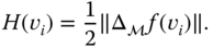
The discrete curvatures can be computed using the discrete Laplace–Beltrami operator as follows:
- The mean curvature:
(2.28)
- The Gaussian curvature at a vertex
 is given as
(2.29)where
is given as
(2.29)where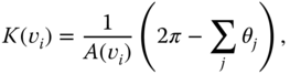
 is the Voronoi area, and
  is the angle between two adjacent edges incident to
  , see Figure 2.10.
 - The principal curvatures:
(2.30)
 (2.31)
2.2 Shape, Shape Transformations, and Deformations
There are several definitions of shape. The most common one is the one that defines shape as the external form, contour, or outline of someone or something. Kendall 7 proposed to study shape as that which is left when the effects associated with translation, isotropic scaling, and rotation are filtered away. This is illustrated in the 2D example of Figure 2.11 where although the five plant leaves have different scales and orientations, they all represent the same leaf shape.
Kendall's definition sets the foundation of shape analysis. It implies that when comparing the shape of two objects, whether they are 2D or 3D, the criteria for comparison should be invariant to shape‐preserving transformations, which are translation, rotation, and scale. It should, however, quantify the deformations that affect shape. For instance, 3D objects can bend, e.g. a walking person, stretch, e.g. a growing anatomical organ, or even change their topology, e.g. an eroding bone, or structure, e.g. a growing tree. In this section, we will formulate these transformations and deformations. The subsequent chapters of the book will show how the Kendall's definition is taken into account in almost every shape analysis framework and task.

Figure 2.11Similarity transformations: examples of 2D objects with different orientations, scales, and locations, but with identical shapes.
2.2.1 Shape‐Preserving Transformations
Let ![]() be the space of all surfaces
be the space of all surfaces ![]() defined by their parametric function of the form
defined by their parametric function of the form ![]() . There are three transformations that can be applied to a surface
. There are three transformations that can be applied to a surface ![]() without changing its shape.
without changing its shape.
- Translation. Translating the surface
 with a displacement vector
  will produce another surface
  such that:
(2.32)
such that:
(2.32)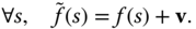
With a slight abuse of notation, we sometimes write
 .
. - Scale. Uniformly scaling the surface
 with a factor
  will produce another surface
  such that:
(2.33)
such that:
(2.33)
- Rotation. A rotation is a
 matrix
  . When applied to a surface
  , we obtain another surface
  such that:

With a slight abuse of notation, we write
 .
.
In the field of shape analysis, the transformations associated with translation, rotation, and uniform scaling are termed shape‐preserving. They are nuisance variables, which should be discarded. This process is called normalization. Normalization for translation and scale is probably the easiest one to deal with. Normalization for rotation requires a more in‐depth attention.
2.2.1.1 Normalization for Translation
One can discard translation by translating ![]() so that its center of mass is located at the origin:
so that its center of mass is located at the origin:
where ![]() is the center of mass of
is the center of mass of ![]() . It is computed as follows:
. It is computed as follows:
Here ![]() is the local surface area at
is the local surface area at ![]() . It is defined as the norm of the normal vector to the surface at
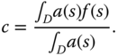
. It is defined as the norm of the normal vector to the surface at ![]() . In the case of objects represented as a set of vertices
. In the case of objects represented as a set of vertices ![]() and faces
and faces ![]() , then the center of mass
, then the center of mass ![]() is given by:
is given by:
Here, ![]() 's are weights associated to each vertex
's are weights associated to each vertex ![]() . One can assume that all vertices have the same weight and set
. One can assume that all vertices have the same weight and set ![]() . This is a simple solution that works fine when the surfaces are densely sampled. A more efficient choice is to set
. This is a simple solution that works fine when the surfaces are densely sampled. A more efficient choice is to set ![]() to be the Voronoi area around the vertex
to be the Voronoi area around the vertex ![]() .
.
2.2.1.2 Normalization for Scale
The scale component can be discarded in several ways. One approach is to scale each 3D object being analyzed in such a way that its overall surface area is equal to one:
where ![]() is a scaling factor chosen to be the entire surface area:
is a scaling factor chosen to be the entire surface area: ![]() . When dealing with triangulated surfaces,
. When dealing with triangulated surfaces, ![]() is chosen to be the sum of the areas of the triangles which form the mesh.
is chosen to be the sum of the areas of the triangles which form the mesh.
Another approach is to scale the 3D object in such a way that the radius of its bounding sphere is equal to one. This is usually done in two steps. First, the 3D object is normalized for translation. Then, it is scaled by a factor ![]() where
where ![]() is the distance between the origin and the farthest point
is the distance between the origin and the farthest point ![]() on the surface from the origin.
on the surface from the origin.
2.2.1.3 Normalization for Rotation
Normalization for rotation is the process of aligning all the 3D models being analyzed in a consistent way. This step is often used after normalizing the shapes for translation and scale. Thus, in what follows, we assume that the 3D models are centered at the origin. There are several ways for rotation normalization. The first approach is to compute the principal directions of the object and then rotate it in such a way that these directions coincide with the three axes of the coordinate system. The second one is more elaborate and uses reflection symmetry planes.
Rotation Normalization Using Principal Component Analysis (PCA)
The first step is to compute the ![]() covariance matrix
covariance matrix ![]() :
:
where ![]() is the number of points sampled on the surface
is the number of points sampled on the surface ![]() of the 3D object,
of the 3D object, ![]() is its center of mass, and
is its center of mass, and ![]() refers to the transpose of the matrix
refers to the transpose of the matrix ![]() . For 3D shapes that are normalized for translation,
. For 3D shapes that are normalized for translation, ![]() is the origin. When dealing with surfaces represented as polygonal meshes, Eq. (2.38) is reduced to
is the origin. When dealing with surfaces represented as polygonal meshes, Eq. (2.38) is reduced to

Here, ![]() is the number of vertices in
is the number of vertices in ![]() . Let
. Let ![]() be the eigenvalues of
be the eigenvalues of ![]() , ordered from the largest to the smallest, and
, ordered from the largest to the smallest, and ![]() their associated eigenvectors (of unit length). Rotation normalization is the process of rotating the 3D object such that the first principal axis,
their associated eigenvectors (of unit length). Rotation normalization is the process of rotating the 3D object such that the first principal axis, ![]() , coincides with the
, coincides with the ![]() axis, the second one,
axis, the second one, ![]() , coincides with the
, coincides with the ![]() axis, and the third one,
axis, and the third one, ![]() , coincides with the
, coincides with the ![]() axis. Note, however, that both
axis. Note, however, that both ![]() and
and ![]() are correct principal directions. To select the appropriate one, one can set the positive direction to be the one that has maximum volume of the shape. Once this is done, then the 3D object can be normalized for rotation by rotating it with the rotation matrix
are correct principal directions. To select the appropriate one, one can set the positive direction to be the one that has maximum volume of the shape. Once this is done, then the 3D object can be normalized for rotation by rotating it with the rotation matrix ![]() that has the unit‐length eigenvectors as rows, i.e.:
that has the unit‐length eigenvectors as rows, i.e.:

Figure 2.12PCA‐based normalization for translation, scale, and rotation of 3D objects that undergo nonrigid deformations.

Figure 2.13PCA‐based normalization for translation, scale, and rotation‐of partial 3D scans. The 3D model is courtesy of SHREC'15: Range Scans based 3D Shape Retrieval 8.
This simple and fast procedure has been extensively used in the literature. Figure 2.12 shows a few examples of 3D shapes normalized using this approach. This figure also shows some of the limitations. For instance, in the case of 3D human body shapes, Principal Component Analysis (PCA) produces plausible results when the body is in a neutral pose. The quality of the alignment, however, degradates with the increase in complexity of the nonrigid deformation that the 3D shape undergoes. The cat example of Figure 2.12 also illustrates another limitation of the approach. In fact, PCA‐based normalization is very sensitive to outliers in the 3D object and to nonrigid deformations of the object's extruded parts such as the tail and legs of the cat. As shown in Figure 2.13, PCA‐based alignment is also very sensitive to geometric and topological noise and often fails to produce plausible alignments when dealing with partial and incomplete data.
In summary, while PCA‐based alignment is simple and fast, which justifies the popularity of the method, it can produce implausible results when dealing with complex 3D shapes (e.g. shapes which undergo complex nonrigid deformations, partial scans with geometrical and topological noise). Thus, objects with a similar shape can easily be misaligned using PCA. This misalignment can result in an exaggeration of the difference between the objects, which in turn will affect the subsequent analysis tasks such as similarity estimation and registration.
Rotation Normalization Using Planar Reflection Symmetry Analysis
PCA does not always produce compatible alignments for objects of the same class. It certainly does not produce alignments similar to what a human would select 9. Podolak et al. 9 used the planar‐reflection symmetry transform (PRST) to produce better alignments. Specifically, they introduced two new concepts, the principal symmetry axes (PSA) and the Center of Symmetry (COS), as robust global alignment features of a 3D model. Intuitively, the PSA are the normals of the orthogonal set of planes with maximal symmetry. In 3D, there are three of such planes. The Center of Symmetry is the intersection of those three planes. The first principal symmetry axis is defined as the plane with maximal symmetry. The second axis can be found by searching for the plane with maximal symmetry among those that are perpendicular to the first one. Finally, the third axis is found in the same way by searching only the planes that are perpendicular to both the first and the second planes of symmetry.

Figure 2.14Comparison between (a) PCA‐based normalization, and (b) planar‐reflection symmetry‐based normalization of 3D shapes.
Source: Image courtesy of http://gfx.cs.princeton.edu/pubs/Podolak_2006_APS/Siggraph2006.ppt and reproduced here with the permission of the authors.
We refer the reader to 9 for a detailed description of how the planar‐reflection symmetry is computed. Readers interested in the general topic of symmetry analysis of 3D models are referred to the survey of Mitra et al. 10 and the related papers. Figure 2.14 compares alignments produced using (a) PCA and (b) planar reflection symmetry analysis. As one can see, the latter produces results that are more intuitive. More importantly, the latter method is less sensitive to noise, missing parts, and extruded parts.
2.2.2 Shape Deformations
In addition to shape‐preserving transformations, 3D objects undergo many other deformations that change their shapes. Here, we focus on full elastic deformations, which we further decompose into the bending and the stretching of the surfaces. Let ![]() and
and ![]() be two parameterized surfaces, which are normalized for translation and scale, and
be two parameterized surfaces, which are normalized for translation and scale, and ![]() the parameterization domain. We assume that
the parameterization domain. We assume that ![]() deforms onto
deforms onto ![]() .
.

Figure 2.15Example of nonrigid deformations that affect the shape of a 3D object. A 3D object can bend, and/or stretch. The first one is referred to as isometric deformations. Fully elastic shapes can, at the same time, bend and stretch.
2.2.3 Bending
Bending, also known as isometric deformation, is a type of deformations that preserves the intrinsic properties (areas, curve lengths) of a surface. During the bending process, the distances along the surface between the vertices are preserved. To illustrate this, consider the 3D human model example of Figure 2.15. When the model bends its arms or legs, the length of the curves along the surface do not change. There are, however, two properties that change. The first one is the angle between, or the relative orientation of, the normal vectors of adjacent vertices. The second one is the curvature at each vertex. As described in Section 2.1.2, normals and curvatures are encoded in the shape operator ![]() . Hence, to quantify bending, one needs to look at how the shape operator changes when a surface deforms isometrically. This can be done by defining an energy function
. Hence, to quantify bending, one needs to look at how the shape operator changes when a surface deforms isometrically. This can be done by defining an energy function ![]() , which computes distances between shape operators, i.e.:
, which computes distances between shape operators, i.e.:

where ![]() denotes the Frobenius norm of a matrix, which is defined for a matrix
denotes the Frobenius norm of a matrix, which is defined for a matrix ![]() of elements
of elements ![]() as
as ![]() .
. ![]() is the shape operation of
is the shape operation of ![]() at
at ![]() .
.
The energy of Eq. (2.41) takes into account the full change in the shape operator. Heeren et al. 11 and Windheuser et al. 12 simplified this metric by only considering changes in the mean curvature, which is the trace of the shape operator:

This energy is also known as the Willmore energy. In the discrete setup, Heeren et al. 13 approximated the mean curvature by the dihedral angle, i.e. the angle between the normals of two adjacent faces on the triangulated mesh.
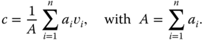
Another way of quantifying bending is to look at changes in the orientation of the normal vectors of the surface during its deformation. Let ![]() be the unit normal vector to the surface
be the unit normal vector to the surface ![]() at
at ![]() . Let also
. Let also ![]() be an infinitesimal perturbation of this normal vector. The magnitude of this perturbation is a natural measure of the strength of bending. It can be defined in terms of inner products as follows:
be an infinitesimal perturbation of this normal vector. The magnitude of this perturbation is a natural measure of the strength of bending. It can be defined in terms of inner products as follows:
2.2.4 Stretching
When stretching a surface ![]() , there are two geometric properties of the surface that change, see Figure 2.15. The first one is the length of the curves along the surface. Consider two points
, there are two geometric properties of the surface that change, see Figure 2.15. The first one is the length of the curves along the surface. Consider two points ![]() and
and ![]() on
on ![]() . Consider also a curve on the surface that connects these two points. Unlike bending, when stretching the surface, the length of this curve changes. The second property that changes is the local surface area at each surface point.
. Consider also a curve on the surface that connects these two points. Unlike bending, when stretching the surface, the length of this curve changes. The second property that changes is the local surface area at each surface point.
Both curve lengths and surface areas are encoded in the first fundamental form ![]() , or metric, of the surface at each point
, or metric, of the surface at each point ![]() . Formally, let
. Formally, let ![]() be a surface and
be a surface and ![]() a stretched version of
a stretched version of ![]() . Let also
. Let also ![]() be the first fundamental form of
be the first fundamental form of ![]() at
at ![]() . The quantity
. The quantity ![]() , called the Cauchy–Green strain tensor, accounts for changes in the metric between the source and the target surfaces. In particular, the trace of the Cauchy–Green strain tensor,
, called the Cauchy–Green strain tensor, accounts for changes in the metric between the source and the target surfaces. In particular, the trace of the Cauchy–Green strain tensor, ![]() , accounts for the local changes in the curve lengths while its determinant,
, accounts for the local changes in the curve lengths while its determinant, ![]() , accounts for the local changes in the surface area 14. Wirth et al. 15, Heeren et al. 11, 16, Berkels et al. 17, and Zhang et al. 14 used this concept to define a measure of stretch between two surfaces
, accounts for the local changes in the surface area 14. Wirth et al. 15, Heeren et al. 11, 16, Berkels et al. 17, and Zhang et al. 14 used this concept to define a measure of stretch between two surfaces ![]() and
and ![]() as
as ![]() where:
where:

Here, ![]() and
and ![]() are constants that balance the importance of each term of the stretch energy. The
are constants that balance the importance of each term of the stretch energy. The ![]() term (the third term) penalizes shape compression.
term (the third term) penalizes shape compression.
Jermyn et al. 18, on the other hand, observed that stretch can be divided into two components; a component which changes the area of the local patches, and a component which changes the shape of the local patches while preserving their areas and the orientation of their normal vectors. These quantities can be captured by looking at small perturbations of the first fundamental form of the deforming surface. Let ![]() be an infinitesimal perturbation of
be an infinitesimal perturbation of ![]() . Then, stretch can be quantified as the magnitude of this perturbation, which can be defined using inner products as follows:
. Then, stretch can be quantified as the magnitude of this perturbation, which can be defined using inner products as follows:
The first term of Eq. (2.45) accounts for changes in the shape of a local patch that preserve the patch area. The second term quantifies changes in the area of these patches. ![]() and
and ![]() are positive values that balance between the importance of each term.
are positive values that balance between the importance of each term.
Finally, one can also measure stretch by taking the difference between the first fundamental forms of the original surface ![]() and its stretched version
and its stretched version ![]() :
:

where ![]() refers to the Frobenius norm and the integration is over the parameterization domain.
refers to the Frobenius norm and the integration is over the parameterization domain.
2.3 Summary and Further Reading
This chapter covered the important fundamental concepts of geometry and topology, differential geometry, transformations and deformations, and the data structures used for storing and processing 3D shapes. These concepts will be extensively used in the subsequent chapters of the book.
The first part, i.e. the elements of differential geometry, will be extensively used in Chapters and 5 to extract geometrical features and build descriptors for the analysis of 3D shapes. They will be also used to model deformations, which are essential for the analysis of 3D shapes which undergo rigid and elastic deformations (Chapters and 7). The concepts of manifolds, metrics, and geodesics, covered in this part, have been used in two ways. For instance, one can treat the surface of a 3D object as a manifold equipped with a metric. Alternatively, one can see the entire space of shapes as a (Riemannian) manifold equipped with a proper metric and a mechanism for computing geodesics. Geodesics in this space correspond to deformations of shapes. These will be covered in detail in Chapter 7, but we also refer the reader to 19 for an in‐depth description of the Riemannian geometry for 3D shape analysis.
The second part of this chapter covered shape transformations and deformations. It has shown how to discard, in a preprocessing step, some of the transformations that are shape‐preserving. As we will see in the subsequent chapters, this preprocessing step is required in many shape analysis algorithms. We will see also that, in some situations, one can design descriptors that are invariant to some of these transformations and thus one does not need to discard them at the preprocessing stage.
Finally, this chapter can serve as a reference for the reader. We, however, refer the readers who are interested in other aspects of 3D digital geometry to the rich literature of digital geometry processing such as 1, 19, 20.
The 3D models used in this chapter have been kindly made available by various authors. For instance, the 3D human body shapes used in Figures 2.12 and 2.15 are courtesy of 21, the 3D cat models are part of the TOSCA database 22, and the partial 3D scans of Figure 2.13 are courtesy of 8.