12
3D Shape Retrieval
12.1 Introduction
The need for efficient 3D search engines is mainly motivated by the large number of 3D models that are being created by novice and professional users, used and stored in public and in private domains, and shared at large scale. In a nutshell, a 3D search engine has the same structure as any image and text search engine. In an offline step, all the 3D models in a collection are indexed by computing, for each 3D model, a set of numerical descriptors which represent uniquely their shape. This is the feature extraction stage. (For details about 3D shape description methods, we refer the reader to Chapters and 5.) The 3D models that are similar in shape should have similar descriptors, while the 3D models that differ in shape should have different descriptors. At runtime, the user specifies a query. The system then ranks the models in the collection according to the distances computed between their descriptors and the descriptor(s) of the query and returns the top elements in the ranked list. This is the similarity computation stage.
In general, the query can have different forms; the user can, for instance, type a set of keywords, draw (a set of) 2D sketch(es), use a few images, or even use another 3D model. We refer to the first three cases as cross‐domain retrieval since the query lies in a domain that is different from the domain of the indexed 3D models. This will be covered in Chapter 13. In this chapter, we focus on the tools and techniques that have been developed for querying 3D model collections using another 3D model as a query. In general, these techniques aim to address two types of challenges. The first type of challenges is similar to what is currently found in text and image search engines and it includes:
- The concept of similarity. The user conception of similarity between objects is often different from the mathematical formulation of distances. It may even differ between users and applications.
- Shape variability in the collection. For instance, 3D shape repositories contain many classes of shapes. Some classes may have a large intra‐class shape variability, while others may exhibit a low inter‐class variability.
- Scalability. The size of the collection that is queried can be very large.
The second type of challenges is specific to the raw representation of 3D objects and the transformations that they may undergo. Compared to (2D) images, the 3D representation of objects brings an additional dimension, which results in more transformations and deformations. These can be:
- Rigid. The rigid transformations include translation, scale and rotation. An efficient shape retrieval method should be invariant to this type of transformations (see Chapter 2 for information about shape‐preserving transformations).
- Nonrigid. 3D objects can also undergo nonrigid deformations, i.e. by bending and stretching their parts (see the examples of Figure 7.1). Some users may require search engines that are invariant to some types of nonrigid deformations, e.g. bending. For example, one may search for 3D human body models of the same person independently of their pose. In that case, the descriptors and similarity metrics for the retrieval should be invariant to this type of deformations.
- Geometric and topological noise. These types of noise are common not only in 3D models that are captured by 3D scanning devices but also in 3D models created using 3D modeling software. In the example of Figure 12.1, the shape of the hand may undergo topological deformations by connecting the thumb and index fingers. In that case, a hole appears and results in a change of the topology of the hand. An efficient retrieval method should not be affected by this type of deformations.
- Partial data. Often, users may search for complete 3D objects using queries with missing parts. This is quite common in cultural heritage where the user searches for full 3D models with parts that are similar to artifacts found at historical sites.

Figure 12.1Some examples of topological noise. When the arm of the 3D human touches the body of the foot, the tessellation of the 3D model changes and results in a different topology. All the models, however, have the same shape (up to isometric deformations) and thus a good 3D retrieval system should be invariant to this type of topological noise. The 3D models are from the SHREC'2016 dataset 414.
To address these challenges, several techniques have been proposed in the literature. Most of them differ by the type of features, which are computed on the 3D models, the way these features are aggregated into descriptors, and the metrics and mechanisms used to compare the descriptors. A common pipeline of the state‐of‐the‐art approaches is given in Figure 12.2. Early works use handcrafted global descriptors (see Chapter 4) and simple similarity measures. While they are easy to compute and utilize, global descriptors are limited to the coarse analysis and comparison of 3D shapes. Their usage is also limited to search in small databases.
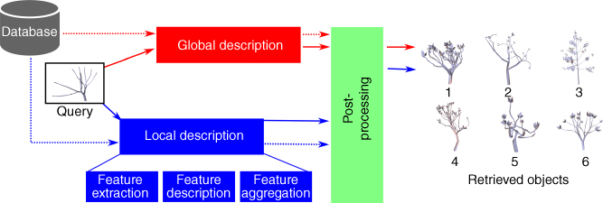
Figure 12.2Global and local‐based 3D shape retrieval pipelines. Dashed lines indicate the offline processes while solid lines indicate online processes.
Handcrafted local descriptors, which have been covered in Chapter , are particularly suitable for the registration and alignment of 3D models. They can also be used for 3D shape retrieval either by one‐to‐one comparison of the local descriptors after registration 415, or by aggregating them using histogram‐like techniques such as bag of words (BoW) 154, or spatially‐sensitive BoWs 123. Aggregation methods have been discussed in Section 5.5. The performance of handcrafted global and local descriptors in 3D shape retrieval will be discussed in Section 12.4.1.
Recently, motivated by their success in many image analysis tasks, deep learning methods are gaining in popularity. In this category of methods, features and the similarity measure are jointly learned from training data. This allows to discard the domain expert knowledge needed when using handcrafted features. Another important advantage of deep learning‐based methods is their scalability, i.e. their ability to handle very large collections of 3D models. These methods will be discussed in Section 12.4.2.
Central to every 3D shape retrieval algorithm is a mechanism for computing distances, dissimilarities, or similarities between descriptors. Different similarity measures can lead to different performances even when using the same type of descriptor. Some of the similarity measures that have been used in the literature will be discussed in Section 12.3.
12.2 Benchmarks and Evaluation Criteria
Before describing the 3D shape retrieval techniques in detail, we will first describe the different datasets and benchmarks, which are currently available in the public domain. We will also present the metrics used to evaluate the quality and performance of a 3D retrieval algorithm. These will enable the reader to compare, in a quantitative manner, the different approaches.
12.2.1 3D Datasets and Benchmarks
There are several 3D model datasets and benchmarks that can be used to evaluate the performance of 3D shape retrieval algorithms. Some datasets have been designed to evaluate how retrieval algorithms perform on generic 3D objects. Others focus on more specific types of objects, e.g. those which undergo nonrigid deformations. Some benchmarks target partial retrieval tasks. In this case, queries are usually parts of the models in the database. Early benchmarks are of a small size (usually less than 10K models). Recently, there have been many attempts to test how 3D algorithms scale to large datasets. This has motivated the emergence of large‐scale 3D benchmarks. Below, we discuss some of the most commonly used datasets.
- The Princeton Shape Benchmark (PSB) 53 is probably one of the most commonly used benchmarks. It provides a dataset of 1814 generic 3D models, stored in the Object File Format (.off), and a package of software tools for performance evaluation. The dataset comes with four classifications, each representing a different granularity of grouping. The base (or finest) classification contains 161 shape categories.
- TOSCA 416 is designed to evaluate how different 3D retrieval algorithms perform on 3D models which undergo isometric deformations (i.e. bending and articulated motion). This database consists of 148 models grouped into 12 classes. Each class contains one 3D shape but in different poses (1–20 poses per shape).
- The McGill 3D Shape Benchmark 417 emphasizes on including models with articulating parts. Thus, whereas some models have been adapted from the PSB, and others have been downloaded from different web repositories, a substantial number have been created by using CAD modeling tools. The 320 models in the benchmark come under two different representations: voxelized form and mesh form. In the mesh format, each object's surface is provided in a triangulated form. It corresponds to the boundary voxels of the corresponding voxel representation. They are, therefore, “jagged” and may need to be smoothed for some applications. The models are organized into two sets. The first one contains objects with articulated parts. The second one contains objects with minor or no articulation motion. Each set has a number of basic shape categories with typically 20–30 models in each category.
- The Toyohashi Shape Benchmark (TSB) 418 is among the first large‐scale datasets which have been made publicly available. This benchmark consists of 10 000 models manually classified into 352 different shape categories.
- SHREC 2014 – Large Scale 80 is one of the first attempts to benchmark large‐scale 3D retrieval algorithms. The dataset contains 8978 models grouped into 171 different shape categories.
- ShapeNetCore 419 consists of 51 190 models grouped into 55 categories and 204 subcategories. The models are further split between training (
 or 35 765 models), testing (
 or 10 266 models), and validation (
 or 5 159 models). The database also comes in two versions. In the normal version, all the models are upright and front orientated. On the perturbed version, all the models are randomly rotated.
 - ShapeNetSem 419 is a smaller, but more densely annotated, subset of ShapeNetCore, consisting of 12 000 models spread over a broader set of 270 categories. In addition, models in ShapeNetSem are annotated with real‐world dimensions, and are provided with estimates of their material composition at the category level, and estimates of their total volume and weight.
- ModelNet 73 is a dataset of more than 127 000 CAD models grouped into 662 shape categories. It is probably the largest 3D dataset currently available and is extensively used to train and test deep‐learning networks for 3D shape analysis. The authors of ModelNet also provide a subset, called ModelNet40, which contains 40 categories.
We refer the reader to Table 12.1 that summarizes the main properties of these datasets.
Table 12.1 Some of the 3D shape benchmarks that are currently available in the literature.
| Name | No. of models | No. of categories | Type | Training | Testing |
| The Princeton Shape Benchmark 53 | 1 814 | 161 | Generic | 907 | 907 |
| TOSCA 416 | 148 | 12 | Nonrigid | — | — |
| McGill 417 | 320 | 19 | Generic + | — | — |
| Nonrigid | — | — | |||
| The Toyohashi Shape Benchmark 418 | 10 000 | 352 | Generic | — | — |
| SHREC 2014 – large scale 80 | 8 987 | 171 | Generic | — | — |
| ShapeNetCore 75 | 51 190 | 55 | Generic | 35 765 | 10 266 |
| ShapeNetSem 75 | 12 000 | 270 | Generic | — | — |
| Princeton ModelNet 73 | 127 915 | 662 | Generic | — | — |
| Princeton ModelNet40 73 | 12 311 | 40 | Generic | — | — |
The last two columns refer, respectively, to the size of the subsets used for training and testing.
12.2.2 Performance Evaluation Metrics
There are several metrics for the evaluation of the performance of 3D shape descriptors and their associated similarity measures for various 3D shape analysis tasks. In this section, we will focus on the retrieval task, i.e. given a 3D model, hereinafter referred to as the query, the user seeks to find, from a database, the 3D models which are similar to the given query. The retrieved 3D models are then ranked and sorted in an ascending order with respect to their similarity to the query. The retrieved list of models is referred to as the ranked list. The role of the performance metrics is to quantitatively evaluate the quality of this ranked list. Below, we will look in detail to some of these metrics.
Let ![]() be the set of objects in the repository that are relevant to a given query, and let
be the set of objects in the repository that are relevant to a given query, and let ![]() be the set of 3D models that are returned by the retrieval algorithm.
be the set of 3D models that are returned by the retrieval algorithm.
12.2.2.1 Precision
Precision is the ratio of the number of models in the retrieved list, ![]() , which are relevant to the query, to the total number of retrieved objects in the ranked list:
, which are relevant to the query, to the total number of retrieved objects in the ranked list:

where ![]() refers to the cardinality of the set
refers to the cardinality of the set ![]() . Basically, precision measures how well a retrieval algorithm discards the junk that we do not want.
. Basically, precision measures how well a retrieval algorithm discards the junk that we do not want.
12.2.2.2 Recall
Recall is the ratio of the number, in the ranked list, of the retrieved objects that are relevant to the query to all objects in the repository that are relevant to the query:
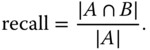
Basically, recall evaluates how well a retrieval algorithm finds what we want.
12.2.2.3 Precision‐Recall Curves
Precision or recall alone are not good indicators of the quality of a retrieval algorithm or a descriptor. For example, one can increase the recall to ![]() by returning all the models in the database. This, however, will decrease the precision. When we perform a search, with any search engine, we are looking to find the most relevant objects (maximizing recall), while minimizing the junk that is retrieved (maximizing precision). The precision‐recall curve measures precision as a function of recall and provides the trade‐off between these two parameters. For a database of
by returning all the models in the database. This, however, will decrease the precision. When we perform a search, with any search engine, we are looking to find the most relevant objects (maximizing recall), while minimizing the junk that is retrieved (maximizing precision). The precision‐recall curve measures precision as a function of recall and provides the trade‐off between these two parameters. For a database of ![]() models, the precision‐recall curve for a query model
models, the precision‐recall curve for a query model ![]() is computed as follows:
is computed as follows:
- First, rank all the
 models in the database in ascending order according to their dissimilarity to the query.
 - For
 , take the first
  elements of the ranked list and then measure both the precision and recall. This gives a point on the precision‐recall curve.
 - Finally, interpolate these points to obtain the precision‐recall curve.
The precision‐recall curve is one of the most commonly used metrics to evaluate 3D model retrieval algorithms.
12.2.2.4 F‐ and E‐Measures
These are two measures that combine precision and recall into a single number to evaluate the retrieval performance. The ![]() ‐measure is the weighted harmonic mean of precision and recall. It is defined as:
‐measure is the weighted harmonic mean of precision and recall. It is defined as:
where ![]() is a weight. When
is a weight. When ![]() , then
, then

The ![]() ‐Measure is defined as
‐Measure is defined as ![]() . Note that the maximum value of the
. Note that the maximum value of the ![]() ‐measure is 1.0 and the higher the
‐measure is 1.0 and the higher the ![]() ‐measure is, the better is the retrieval algorithm. The main property of the
‐measure is, the better is the retrieval algorithm. The main property of the ![]() ‐measure is that it tells how good are the results which have been retrieved in the top of the ranked list. This is very important since, in general, the user of a search engine is more interested in the first page of the query results than in the later pages.
‐measure is that it tells how good are the results which have been retrieved in the top of the ranked list. This is very important since, in general, the user of a search engine is more interested in the first page of the query results than in the later pages.
12.2.2.5 Area Under Curve (AUC) or Average Precision (AP)
By computing the precision and recall at every position in the ranked list of 3D models, one can plot the precision as a function of recall. The average precision (AP) computes the average value of the precision over the interval from ![]() to
to ![]() :
:

where ![]() refers to recall. This is equivalent to the area under the precision‐recall curve.
refers to recall. This is equivalent to the area under the precision‐recall curve.
12.2.2.6 Mean Average Precision (mAP)
Mean average precision (mAP) for a set of queries is the mean of the AP scores for each query:
where ![]() is the number of queries and AP
is the number of queries and AP![]() is the AP of the query
is the AP of the query ![]() .
.
12.2.2.7 Cumulated Gain‐Based Measure
This is a statistic that weights the correct results near the front of the ranked list more than the correct results that are down in the ranked list. It is based on the assumption that a user is less likely to consider elements near the end of the list. Specifically, a ranked list ![]() is converted to a list
is converted to a list ![]() . An element
. An element ![]() has a value of 1 if the element
has a value of 1 if the element ![]() is in the correct class and a value of 0 otherwise. The cumulative gain
is in the correct class and a value of 0 otherwise. The cumulative gain ![]() is then defined recursively as follows:
is then defined recursively as follows:

The discounted cumulative gain (DCG), which progressively reduces the object weight as its rank increases but not too steeply, is defined as:
We are usually interested in the NDCG, which scales the DCG values down by the average, over all the retrieval algorithms which have been tested, and shifts the average to zero:
where NDCGA is the normalized DCG for a given algorithm ![]() , DCGA is the DCG value computed for the algorithm
, DCGA is the DCG value computed for the algorithm ![]() , and AvgDCG is the average DCG value for all the algorithms being compared in the same experiment. Positive/negative normalized DCG scores represent the above/below average performance, and the higher numbers are better.
, and AvgDCG is the average DCG value for all the algorithms being compared in the same experiment. Positive/negative normalized DCG scores represent the above/below average performance, and the higher numbers are better.
12.2.2.8 Nearest Neighbor (NN), First‐Tier (FT), and Second‐Tier (ST)
These performance metrics share a similar idea, that is, to check for the ratio of models in the query's class, which appear within the top ![]() matches. In the case of the nearest neighbor (NN) measure,
matches. In the case of the nearest neighbor (NN) measure, ![]() is set to 1. It is set to the size of the query's class for the first‐tier (FT) measure, and to twice the size of the query's class for second‐tier (ST).
is set to 1. It is set to the size of the query's class for the first‐tier (FT) measure, and to twice the size of the query's class for second‐tier (ST).
These measures are based on the assumption that each model in the dataset has only one ground truth label. In some datasets, e.g. the ShapeNetCore 419, a model can have two groundtruth labels (one for the category and another for the subcategory). In this case, one can define a modified version of the NDCG metric that uses four levels of relevance:
- Level 3 corresponds to the case where the category and subcategory of the retrieved shape perfectly match the category and subcategory of the query.
- Level 2 corresponds to the case where both the category and subcategory of the retrieved 3D shape are the same as the category of the query.
- Level 1 corresponds to the case where the category of the retrieved shape is the same as the category of the query, but their subcategories differ.
- Level 0 corresponds to the case where there is no match.
Meanwhile, since the number of shapes in different categories is not the same, the other evaluation metrics (MAP, ![]() ‐measure and NDCG) will also have two versions. The first one, called macro‐averaged version, is used to give an unweighted average over the entire dataset. The second one, called micro‐averaged version, is used to adjust for model category sizes, which results in a representative performance metric averaged across categories. To ensure a straightforward comparison, the arithmetic mean of macro version and micro version is also used.
‐measure and NDCG) will also have two versions. The first one, called macro‐averaged version, is used to give an unweighted average over the entire dataset. The second one, called micro‐averaged version, is used to adjust for model category sizes, which results in a representative performance metric averaged across categories. To ensure a straightforward comparison, the arithmetic mean of macro version and micro version is also used.
12.3 Similarity Measures
Retrieval algorithms are based on similarity search, i.e. they compute the similarity of the query's descriptor to the descriptors of the models in the database. There are several methods that have been used to compute such similarity. Here, we will look at three classes of methods. The first class of methods use standard distance measures (Section 12.3.1). The second class of methods use Hamming distances on hash codes (Section 12.3.2). The final class of methods use manifold ranking techniques (Section 12.3.3).
12.3.1 Dissimilarity Measures
Table 12.2 lists a selection of 12 measures used for 3D shape retrieval. When the measure is a distance, then the models in the database are ranked in ascending order of their distance to the query. When the measure is a similarity, then the models are ranked in a descending order of their similarity to the query.
Table 12.2 A selection of ![]() distance measures used in 3D model retrieval algorithms.
distance measures used in 3D model retrieval algorithms.
| Name | Type | Measure |
| City block ( |
Distance |  |
| Euclidean ( |
Distance | 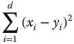 |
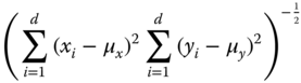
| Canberra metric | Distance | 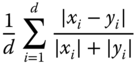 |
| Divergence coefficient | Distance | 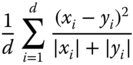 |
| Correlation coefficient | Similarity | 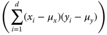 |
 |
||
| Profile coefficient | Similarity |  |
| Intraclass coefficient | Similarity |  . . |
| Catell 1949 | Similarity | 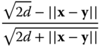 |
| Angular distance | Similarity | 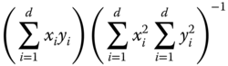 |
| Meehl index | Distance |  |
| Kappa | Distance | 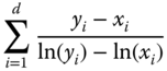 |
| Inter‐correlation coefficient | Similarity |  |
 |
Here, ![]() and
and ![]() are two descriptors,
are two descriptors, ![]() is the size, or dimension, of the descriptors,
is the size, or dimension, of the descriptors,  ,
,  ,
,  ,
,  ,
,  ,
, ![]() .
.
12.3.2 Hashing and Hamming Distance
Hashing is the process of encoding high‐dimensional descriptors as similarity‐preserving compact binary codes (or strings). This can enable large efficiency gains in storage and computation speed when performing similarity search such as the comparison of the descriptor of a query to the descriptors of the elements in the data collection being indexed. With binary codes, similarity search can also be accomplished with much simpler data structures and algorithms, compared to alternative large‐scale indexing methods 420.
Assume that we have a set of ![]() data points
data points ![]() where each point is a descriptor of a 3D shape, and
where each point is a descriptor of a 3D shape, and ![]() is the dimensionality of the descriptors, which can be very large. We also assume that
is the dimensionality of the descriptors, which can be very large. We also assume that ![]() is a column vector. Let
is a column vector. Let ![]() be a
be a ![]() matrix whose
matrix whose ![]() th row is set to be
th row is set to be ![]() for every
for every ![]() . We assume that the points are zero centered, i.e.
. We assume that the points are zero centered, i.e. ![]() where
where ![]() is the vector whose elements are all set to 0. The goal of hashing is to learn a binary code matrix
is the vector whose elements are all set to 0. The goal of hashing is to learn a binary code matrix ![]() , where
, where ![]() denotes the code length. This is a two step process:
denotes the code length. This is a two step process:
- The first step applies linear dimensionality reduction to the data. This is equivalent to projecting the data onto a hyperplane of dimensionality
 , the size of the hash code, using a projection matrix
  of size
  . The new data points are the rows of the
  matrix
  given by:
(12.10)
given by:
(12.10)
Gong et al. 420 obtain the matrix
 by first performing principal component analysis (PCA). In other words, for a code of
  bits, the columns of
  are formed by taking the top
  eigenvectors of the data covariance matrix
  .
. - The second step is a binary quantization step that produces the final hash code
 by taking the sign of
  . That is:
(12.11)where
. That is:
(12.11)where
 if
if  , and 0 otherwise. For a matrix or a vector,
  denotes the result of the element‐wise application of the above sign function. The
  th row of
  represents the final hash code of the descriptor
  .
.
A good code, however, is the one that minimizes the quantization loss, i.e. the distance between the original data points and the computed hash codes. Instead of quantizing directly ![]() , Gong et al. 420 starts by rotating the data points, using a
, Gong et al. 420 starts by rotating the data points, using a ![]() rotation matrix
rotation matrix ![]() , so that the quantization loss:
, so that the quantization loss:
is minimized. (Here ![]() refers to the Frobenius norm.) This can be solved using the iterative quantization (ITQ) procedure, as detailed in 420. That is:
refers to the Frobenius norm.) This can be solved using the iterative quantization (ITQ) procedure, as detailed in 420. That is:
- Fix
 and update
  . Let
. Let  . For a fixed rotation
  , the optimal code
  is given as
  .
. - Fix
 and update
  . For a fixed code
  , the objective function of Eq. 12.12 corresponds to the classic Orthogonal Procrustes problem in which one tries to find a rotation to align one point set to another. In our case, the two point sets are given by the projected data
  and the target binary code matrix
  . Minimizing Eq. 12.12 with respect to
  can be done as follows: first compute the SVD of the
  matrix
  as
as  and then let
  .
.
At runtime, the descriptor ![]() of a given query is first projected onto the hyperplane, using the projection matrix
of a given query is first projected onto the hyperplane, using the projection matrix ![]() , and then quantized to form a hash code
, and then quantized to form a hash code ![]() by taking the sign of the projected point. Finally, the hash code
by taking the sign of the projected point. Finally, the hash code ![]() is compared to the hash codes of the 3D models in the database using the Hamming distance, which is very efficient to compute. In fact, the Hamming distance between two binary codes of equal length is the number of positions at which the corresponding digits are different.
is compared to the hash codes of the 3D models in the database using the Hamming distance, which is very efficient to compute. In fact, the Hamming distance between two binary codes of equal length is the number of positions at which the corresponding digits are different.
Hashing has been extensively used for large‐scale image retrieval 420–424 and has been recently used for large‐scale 3D shape retrieval 425–427.
12.3.3 Manifold Ranking
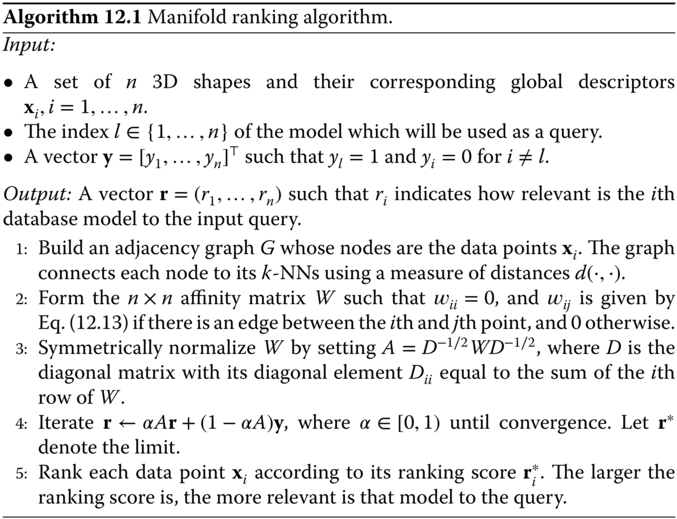
Traditional 3D retrieval methods use distances to measure the dissimilarity of a query to the models in the database. In other words, the perceptual similarity is based on pair‐wise distances. Unlike these methods, manifold ranking 428 measures the relevance between the query and each of the 3D models in the database (hereinafter referred to as data points) by exploring the relationship of all the data points in the feature (or descriptor) space. The general procedure is summarized in Algorithm 12.1. Below, we describe the details.
Consider a set of ![]() 3D shapes and their corresponding global descriptors
3D shapes and their corresponding global descriptors ![]() . Let
. Let ![]() denote the space of such descriptors. Manifold ranking starts by building a graph whose nodes are the 3D shapes (represented by their descriptors), and then connecting each node to its
denote the space of such descriptors. Manifold ranking starts by building a graph whose nodes are the 3D shapes (represented by their descriptors), and then connecting each node to its ![]() ‐NNs in the descriptor space. Each edge
‐NNs in the descriptor space. Each edge ![]() , which connects the
, which connects the ![]() th and
th and ![]() th node, is assigned a weight
th node, is assigned a weight ![]() defined as
defined as

where ![]() is a measure of distance in the descriptor space, and
is a measure of distance in the descriptor space, and ![]() is a user‐specified parameter. We collect these weights into an
is a user‐specified parameter. We collect these weights into an ![]() matrix
matrix ![]() and set
and set ![]() to 0 if there is no edge which connects the
to 0 if there is no edge which connects the ![]() th and
th and ![]() th nodes.
th nodes.
Now, let us define a ranking vector ![]() , which assigns to each point
, which assigns to each point ![]() a ranking score
a ranking score ![]() . Let
. Let ![]() be a vector such that
be a vector such that ![]() if
if ![]() is the query and
is the query and ![]() otherwise. The cost associated with the ranking vector
otherwise. The cost associated with the ranking vector ![]() is defined as:
is defined as:

where ![]() is a regularization parameter and
is a regularization parameter and ![]() is an
is an ![]() diagonal matrix, whose diagonal elements
diagonal matrix, whose diagonal elements  . The first term of Eq. 12.14 is a smoothness constraint. It ensures that adjacent nodes will likely have similar ranking scores. The second term is a fitting constraint to ensure that the ranking result fits to the initial label assignment. If we have more prior knowledge about the relevance or confidence of each query, we can assign different initial scores to the queries.
Finally, the optimal ranking is obtained by minimizing Eq. 12.14, which has a closed‐form solution. That is:
where ![]() ,
, ![]() is the
is the ![]() identity matrix, and
identity matrix, and ![]() .
.
Equation 12.15 requires the computation of the inverse of the square matrix ![]() , which is of size
, which is of size ![]() . When dealing with large 3D datasets (i.e. when
. When dealing with large 3D datasets (i.e. when ![]() is very large), computing such matrix inverse is computationally very expensive. In such cases, instead of using the closed‐form solution, we can solve the optimization problem using an iterative procedure that starts by initializing the ranking
is very large), computing such matrix inverse is computationally very expensive. In such cases, instead of using the closed‐form solution, we can solve the optimization problem using an iterative procedure that starts by initializing the ranking ![]() . Then, at each iteration
. Then, at each iteration ![]() , the new ranking
, the new ranking ![]() is obtained as
is obtained as
This procedure is then repeated until convergence, i.e. ![]() . The ranking score
. The ranking score ![]() of the
of the ![]() th 3D model in the database is proportional to the probability that it is relevant to the query, with large ranking scores indicating a high probability.
th 3D model in the database is proportional to the probability that it is relevant to the query, with large ranking scores indicating a high probability.
12.4 3D Shape Retrieval Algorithms
12.4.1 Using Handcrafted Features
Early works in 3D shape retrieval are based on handcrafted descriptors, which can be global, as described in Chapter , or local but aggregated into global descriptors using bag of features (BoF) techniques, as described in Section 5.5.
The use of global descriptors for 3D shape retrieval is relatively straightforward; in an offline step, a global descriptor is computed and stored for each model in the database. At runtime, the user specifies a query, and the system computes a global descriptor, which is then compared, using some distance measures, to the descriptors of the models in the database.
Table 12.3 summarizes and compares the performance of some global descriptors. These results have been already discussed in some other papers, e.g. 53, 61, 68, but we reproduce them here for completeness. In this experiment, we take the descriptors presented in Sections , and 4.4 and compare their retrieval performance, using the performance metrics that are presented in Section 12.2, on the 907 models of the test set of the PSB 53. We sort the descriptors in a descending order with respect to their performance on the DCG measure. Table 12.3 also shows the distance metrics that have been used to compare the descriptors.
Table 12.3 Performance evaluation of handcrafted descriptors on the test set of the Princeton Shape Benchmark 53.
| Descriptor | Size (bytes) | Distance | NN | FT | ST | DCG | |
| 512 | 0.469 | 0.314 | 0.397 | 0.205 | 0.654 | ||
| LFD 52 | 4 700 | min |
0.657 | 0.38 | 0.487 | 0.280 | 0.643 |
| difference | |||||||
| SWEL1 61 | 76 | 0.373 | 0.276 | 0.359 | 0.186 | 0.626 | |
| REXT 53, 59 | 17 416 | 0.602 | 0.327 | 0.432 | 0.254 | 0.601 | |
| SWEL2 61 | 76 | 0.303 | 0.249 | 0.315 | 0.161 | 0.594 | |
| GEDT 53, 60 | 32 776 | 0.603 | 0.313 | 0.407 | 0.237 | 0.584 | |
| SHD 53, 60, 76 | 2 184 | 0.556 | 0.309 | 0.411 | 0.241 | 0.584 | |
| EXT 53, 58 | 0.549 | 0.286 | 0.379 | 0.219 | 0.562 | ||
| SECSHELLS 51, 53 | 32 776 | 0.546 | 0.267 | 0.350 | 0.209 | 0.545 | |
| D2 48, 429 | 0.311 | 0.158 | 0.235 | 0.139 | 0.434 |
“Distance” refers to the distance measure used to compare the descriptors.
The interesting observation is that, according to the five evaluation metrics used in Table 12.3, the light field descriptor (LFD), which is view‐based, achieves the best performance. The LFD also offers a good trade‐off between memory requirements, computation time, and performance compared to other descriptors such as the Gaussian Euclidean Distance Transform (GEDT) and SHD, which achieve a good performance but at the expense of significantly higher memory requirements. Note also that spherical‐wavelet descriptors, such as ![]() , SWEL1, and SWEL2 (see Section 4.4.2.2), are very compact, achieve good retrieval performance in terms of DCG, but their performance in terms of Nearest Neighbor (NN), First Tier (FT), Second Tier (ST), and
, SWEL1, and SWEL2 (see Section 4.4.2.2), are very compact, achieve good retrieval performance in terms of DCG, but their performance in terms of Nearest Neighbor (NN), First Tier (FT), Second Tier (ST), and ![]() ‐measure (
‐measure (![]() ‐) is relatively low compared to the LFD, REXT, and SHD.
‐) is relatively low compared to the LFD, REXT, and SHD.
Table 12.4 Examples of local descriptor‐based 3D shape retrieval methods and their performance on commonly used datasets.
| PSB 53 | WM‐SHREC07 430 | McGill 417 | |||||||
| Method | NN | FT | ST | NN | FT | ST | NN | FT | ST |
| VLAT coding 431 | — | — | — | — | — | — | 0.969 | 0.658 | 0.781 |
| Cov.‐BoC 139 | — | — | — | 0.930 | 0.623 | 0.737 | 0.977 | 0.732 | 0.818 |
| 2D/3D hybrid 432 | 0.742 | 0.473 | 0.606 | 0.955 | 0.642 | 0.773 | 0.925 | 0.557 | 0.698 |
| CM‐BoF + GSMD 141 | 0.754 | 0.509 | 0.640 | — | — | — | — | — | — |
| CM‐BoF 141 | 0.731 | 0.470 | 0.598 | — | — | — | — | — | — |
| Improved BoC 427 | — | — | — | 0.965 | 0.743 | 0.889 | 0.988 | 0.809 | 0.935 |
| TLC (VLAD) 433 | 0.763 | 0.562 | 0.705 | 0.988 | 0.831 | 0.935 | 0.980 | 0.807 | 0.933 |
Table 12.4 summarizes the performance of some 3D shape retrieval methods that use local descriptors aggregated using BoFs techniques. We can see from Tables 12.3 and 12.4 that local descriptors outperform the global descriptors on benchmarks that contain generic 3D shapes, e.g. the PSB 53 and on datasets that contain articulated shapes (e.g. McGill dataset 417).
An important advantage of local descriptors is their flexibility in terms of the type of analysis that can be performed with. They can be used as local features for shape matching and recognition as shown in Chapters and . They can also be aggregated over the entire shape to form global descriptors as shown in Table 12.4. Also, local descriptors characterize only the local geometry of the 3D shape, and thus they are usually robust to some nonrigid deformations, such as bending and stretching, and to geometric and topological noise.
12.4.2 Deep Learning‐Based Methods
The main issue with the handcrafted (global or local) descriptors is that they do not scale well with the size of the datasets. Table 12.5 shows that the LFD and the SHD descriptors, which are the best performing global descriptors on the PSB, achieved only ![]() and
and ![]() , respectively, of mAP on the ModelNet dataset 73, which contains 127 915 models divided into 662 shape categories. Large 3D shape datasets are in fact very challenging. They often exhibit high inter‐class similarities and also high intraclass variability. Deep learning techniques perform better in such situations since, instead of using handcrafted features, they learn, automatically from training data, the features which achieve the best performance.
, respectively, of mAP on the ModelNet dataset 73, which contains 127 915 models divided into 662 shape categories. Large 3D shape datasets are in fact very challenging. They often exhibit high inter‐class similarities and also high intraclass variability. Deep learning techniques perform better in such situations since, instead of using handcrafted features, they learn, automatically from training data, the features which achieve the best performance.
Table 12.5 Comparison between handcrafted descriptors and Multi‐View CNN‐based descriptors 68 on ModelNet 73.
Source: The table is adapted from 68.
| Training configuration | Test config. | ||||||
| Method | Pretrain | Fine‐tune | #Views | #Views | Classif. accuracy | Retrieval (mAP) | |
| SHD 60, 76 | — | — | — | — | 68.2 | 33.3 | |
| LFD 52 | — | — | — | — | 75.5 | 40.9 | |
| CNN without f.t. | ImageNet1K | — | — | 1 | 83.0 | 44.1 | |
| CNN, with f.t. | ImageNet1K | ModelNet40 | 12 | 1 | 85.1 | 61.7 | |
| MVCNN | ImageNet1K | — | — | 12 | 88.1 | 49.4 | |
| without f.t. | |||||||
| MVCNN, with f.t. | ImageNet1K | ModelNet40 | 12 | 12 | 89.9 | 70.1 | |
| MVCNN | ImageNet1K | — | 80 | 80 | 84.3 | 36.8 | |
| without f.t. | |||||||
| MVCNN with f.t. | ImageNet1K | ModelNet40 | 80 | 80 | 90.1 | 70.4 | |
The pretraining is performed on ImageNet 70. “f.t.” refers to fine‐tuning.
Table 12.5 summarizes the performance, in terms of the classification accuracy and the mAP on the ModelNet benchmark 73, of multiview Convolutional Neural Network‐based global descriptors 68. It also compares them to the standard global descriptors such as SHD and LFD. In this table, CNN refers to the descriptor obtained by training a CNN on a (large) image database, and using it to analyze views of 3D shapes. MVCNN refers to the multi‐view CNN presented in Section 4.5.2. At runtime, one can render a 3D shape from any arbitrary viewpoint, pass it through the pretrained CNN, and take the neuron activations in the second‐last layer as the descriptor. The descriptors are then compared using the Euclidean distance.
To further improve the accuracy, one can fine‐tune these networks (CNN and MVCNN) on a training set of rendered shapes before testing. This is done by learning, in a supervised manner, the dissimilarity function which achieves the best performance. For instance, Su et al. 68 learned a Mahalanobis metric ![]() which directly projects multiview CNN descriptors
which directly projects multiview CNN descriptors ![]() to
to ![]() , such that the
, such that the ![]() distances in the projected space are small between shapes of the same category, and large between 3D shapes that belong to different categories. Su et al. 68 used the large‐margin metric learning algorithm with
distances in the projected space are small between shapes of the same category, and large between 3D shapes that belong to different categories. Su et al. 68 used the large‐margin metric learning algorithm with ![]() ,
, ![]() to make the final descriptor compact.
to make the final descriptor compact.
With this fine‐tuning, CNN descriptors, which use a single view (from an unknown direction) of the 3D shape, outperform the LFD. In fact, the mAP on the 40 classes of the ModelNet 73 improves from ![]() (LFD) to
(LFD) to ![]() . This performance is further boosted to
. This performance is further boosted to ![]() when using the MultiView CNN, with 80 views and with fine‐tuning the CNN training on ImageNet1K.
when using the MultiView CNN, with 80 views and with fine‐tuning the CNN training on ImageNet1K.
Table 12.6 Performance comparison on ShapeNet Core55 normal dataset of some learning‐based methods.
| Micro | Macro | Micro + Macro | |||||||
| Method | mAP | NDCG | mAP | NDCG | mAP | NDCG | |||
| Kanezaki 434 | 0.798 | 0.772 | 0.865 | 0.590 | 0.583 | 0.650 | 0.694 | 0.677 | 0.757 |
| Tatsuma_ReVGG 434 | 0.772 | 0.749 | 0.828 | 0.519 | 0.496 | 0.559 | 0.645 | 0.622 | 0.693 |
| Zhou 434 | 0.767 | 0.722 | 0.827 | 0.581 | 0.575 | 0.657 | 0.674 | 0.648 | 0.742 |
| MVCNN 68 | 0.764 | 0.873 | 0.899 | 0.575 | 0.817 | 0.880 | 0.669 | 0.845 | 0.890 |
| Furuya_DLAN 434 | 0.712 | 0.663 | 0.762 | 0.505 | 0.477 | 0.563 | 0.608 | 0.570 | 0.662 |
| Thermos_ | 0.692 | 0.622 | 0.732 | 0.484 | 0.418 | 0.502 | 0.588 | 0.520 | 0.617 |
| MVFusionNet 434 | |||||||||
| GIFT 82 | 0.689 | 0.825 | 0.896 | 0.454 | 0.740 | 0.850 | 0.572 | 0.783 | 0.873 |
| Li and coworkers 419 | 0.582 | 0.829 | 0.904 | 0.201 | 0.711 | 0.846 | 0.392 | 0.770 | 0.875 |
| Deng_CM‐ | 0.479 | 0.540 | 0.654 | 0.166 | 0.339 | 0.404 | 0.322 | 0.439 | 0.529 |
| VGG5‐6DB 434 | |||||||||
| Tatsuma and Aono 435 | 0.472 | 0.728 | 0.875 | 0.203 | 0.596 | 0.806 | 0.338 | 0.662 | 0.841 |
| Wang and coworkers 419 | 0.391 | 0.823 | 0.886 | 0.286 | 0.661 | 0.820 | 0.338 | 0.742 | 0.853 |
| Mk_DeepVoxNet 434 | 0.253 | 0.192 | 0.277 | 0.258 | 0.232 | 0.337 | 0.255 | 0.212 | 0.307 |
Here, ![]() ‐refers to the
‐refers to the ![]() ‐measure; VLAD stands for vector of locally aggregated descriptors.
‐measure; VLAD stands for vector of locally aggregated descriptors.
Table 12.6 summarizes the performance, in terms of the ![]() ‐measure, mAP, and NDCG, of some other deep learning‐based methods. Overall, the retrieval performance of these techniques is fairly high. In fact, most of the learning‐based methods outperform traditional handcrafted features‐based approaches.
‐measure, mAP, and NDCG, of some other deep learning‐based methods. Overall, the retrieval performance of these techniques is fairly high. In fact, most of the learning‐based methods outperform traditional handcrafted features‐based approaches.
12.5 Summary and Further Reading
In this chapter, we discussed how shape descriptors and similarity measures are used for 3D shape retrieval. We focused on the case where the user specifies a complete 3D model as a query. The retrieval system then finds, from a collection of 3D models, the models that are the most relevant to the query.
The field of 3D model retrieval has a long history, which we can summarize in three major eras. The methods in the first era used the handcrafted global descriptors described in Chapter 4. Their main focus was on designing descriptors that capture the overall properties of shapes while achieving invariance to rigid transformations (translation, scaling, and rotation).
Methods in the second era used local descriptors aggregated into global descriptors using aggregation techniques such as the BoF. Their main focus was on achieving (i) invariance to rigid transformations and isometric (bending) deformations, (ii) robustness to geometrical and topological noise, and incomplete data (as is the case with 3D scans), and (iii) better retrieval performance.
The new era of 3D shape retrieval tackled the scalability problem. Previous methods achieved relatively acceptable results only on small datasets. Their performance drops significantly when used on large datasets such as ShapeNet 75. This new generation of methods is based on deep learning techniques that achieved remarkable performances on large‐scale image retrieval. Their main limitation, however, is that they require large amounts of annotated training data and a substantial computational power. Although datasets such as the ShapeNet 75 and ModelNet 73 provide annotated data for training, their sizes are still too small compared to existing image collections (in the 100K while image collections are well above millions). Thus, we expect that the next generation of retrieval methods would focus on handling weakly annotated data. We also expect that very large datasets of 3D models will start to emerge in the near future.