Chapter 7: One-Sample Tests
Getting an Intuitive Feel for a One-Sample t Test
Performing a One-Sample t Test
Nonparametric One-Sample Tests
SAS Studio comes equipped with statistical tasks for just about any statistical query that you will need as a student or researcher.
You might have very little need to perform a one-sample test, but let’s start there anyway. Typically, a one-sample test is used to determine if a single sample comes from a population with a known mean. This is in contrast to a two-sample test (discussed in the next chapter), where you want to test if two samples come from populations with different means. This chapter will show you how to navigate the various tabs that are common to all the statistical tasks. You will also see how to test some basic assumptions that need to be met before performing most parametric tests.
Getting an Intuitive Feel for a One-Sample t Test
Before we get into the details of running a one-sample t test, let’s get an intuitive feel for how this test works.
The purpose of a one-sample test is usually to demonstrate that your sample of values comes or does not come from a population whose mean is known. For example, you might have before and after scores for students in a math program. You want to see whether they improved as a result of the program. If the null hypothesis was that the math program had no effect on scores, the mean difference (after – before) of the population from which you took your sample would be 0. Suppose you sample 10 students and the difference scores are as follows:
10 11 9 12 12 10 8 9 10 11
The mean is 10.2. Do you think the math program improved scores? You need to use these scores to estimate a population mean (your best guess would be 10.2, the mean of the sample). You need to determine whether it is unlikely to get a mean of 10.2 from a sample of 10 scores if the true population mean was 0. Your intuition should be that, given these 10 scores, that situation is very unlikely.
A t test is one way to assign a probability that, if the null hypothesis were true, you would obtain a sample mean as large or as small as you got, by chance alone. This is the famous p-value you see reported in almost any study. If the probability is small (usually defined as less than .05), you reject the null hypothesis and accept the alternative hypothesis.
For those curious folks, running a one-sample t test on the 10 difference scores above results in a p-value of less than .0001. The math program worked.
Performing a One-Sample t Test
For this first example of a one-sample t test, we are going to visit a place called Small Town USA. This town has a single school for all grades—kindergarten through high school. Fifteen students in this school took the SAT exam in hopes of going to a quality college. The national average on the combined mathematics and English portions of the SAT is 1068. The 15 scores of the students who took the SAT from the Small Town School were entered into an Excel spreadsheet, as shown in Figure 7.1.
Figure 7.1: SAT Scores from Small Town School (SAT_Scores.xlsx)

The school administrators want to know if their students scored higher than the national average. Even though the mean score for these 15 students was 1270.6, is it possible these students guessed really well on the test? If they were really similar to the rest of the country, what would be the chance of getting such a high mean?
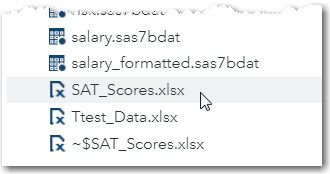
To answer that question, you decide to perform a one-sample t test. The first step is to use the Import Data facility under the Tasks and Utilities tab as described in the previous chapter. Instead of clicking on the Select File box in the Import task, this time, for variety, you click the Server Files and Folders tab, then myfolder, click on the SAT_Scores.xlsx file, and drag it over to the drop and drag area.
Figure 7.2: Selecting Your File in the Server Files and Folders Tab

This brings up the following screen:
Figure 7.3: Importing the SAT_Scores Workbook
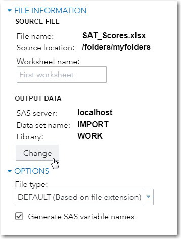
Click Change, name the SAS data set SAT_Scores, and place it in the WORK library.
Remember, all files that you place in the WORK library disappear when you close your SAS session.
You are now ready to run your one-sample t test. Start by expanding Tasks on the navigation pane and then expand the Statistics tab. (See Figure 7.4.)
Figure 7.4: Selecting a One-Sample Test

As with almost every statistical task, the first tab you see is the DATA tab. This tab is where you select the SAS data set that contains your data and select which variables you need for various roles. Figure 7.5 shows the DATA tab for the One-Way task.
Figure 7.5: The DATA Tab for One-Sample Tests

Select the data set SAT_Scores in the WORK library. In the Roles pull-down list, select a One-sample test and the variable SAT_Score as the Analysis variable. The next step is to open the OPTIONS tab (Figure 7.6).
Figure 7.6: The OPTIONS Tab for One-Sample Tests

Because just about every test that you perform is a two-tailed (non-directional) test, you leave that default selection as it is. A two-tailed test can result in a significant result if the sample mean is significantly higher or lower than a hypothesized value. Even though you expect that these students have higher scores than the national average, you still allow for a result that they performed below the average. Next, you specify an Alternative hypothesis that the mean of the population from which you took your sample is not 1068, the national average. You might be more familiar with stating a null hypothesis instead of an alternative hypothesis when conducting one-sample t tests. However, specifying a null hypothesis as mu (the population mean) is equal to 1068 is equivalent to specifying the alternative hypothesis that mu is not equal to 1068. You should also check the box labeled Tests of normality because normality is one of the assumptions for performing a one-sample t test.
You can select which plots you would like the task to display, but for now, leave the selection of Default plots. It is time to run the task, so click the Run icon.
The first table displayed shows the results of four different tests for normality (Figure 7.7 below).
Figure 7.7: Several Tests for Normality
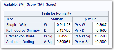
You will see slightly different results from these tests. Some of these tests are more or less likely to reject the null hypothesis that your data came from a population that was normally distributed. In most cases, all (or a majority) of the tests will lead you to the same conclusion. In this example, none of the four tests are significant at the .05 level (the magic number in statistics).
Looking at the p-values from the tests of normality is not sufficient to make a determination that it is OK or not OK to conduct a t test.
Why is this important? (I will repeat this discussion in relation to several other statistical tests later in this book because it is so important.) If you have a very large sample size, all of these tests for normality might be significant, even though your distribution is close to a normal distribution. This is because statistical tests with large sample sizes have more power to detect small differences. If your sample size is small, the tests for normality can often fail to reject the null hypothesis, and it is with small samples that the normality assumption is important.
Here is the problem: Most of the statistical tests that we discuss in this book have as one of their assumptions that you have normally distributed data. However, the central limit theorem states that the sampling distribution will be normally distributed if n, the sample size, is sufficiently large. Your next question should be: What is sufficiently large?
A sample size that is considered sufficiently large depends on the shape of the distribution of values. If the distribution is somewhat symmetrical, sufficiently large might be quite small (10 or 20). If the distribution is highly skewed, sufficiently large might be quite large. Before you decide to abandon the one-sample t test, you should look at the distribution of your scores in a histogram and/or a Q-Q plot. The one-sample t test task produces both of these plots to help you understand how your data values are distributed.
An aside: When I worked as a biostatistician at a medical school in New Jersey, I would consult with researchers, many of whom had some statistical expertise. They would show me output from a test (such as a t test) and point out that the test of normality rejected the null hypothesis and that they could not use a t test (or other parametric test) to analyze their data. My next question would be, “What is your sample size?” Sometimes the answer would be hundreds or thousands. If that is the case, and the distribution as shown by a histogram is mostly symmetrical, you can use the results of the t test (or other test requiring normally distributed data) without any problem.
The next part of the output shows the mean and standard deviation along with several other statistics. Of particular interest are the t value and the probability of a type I error.
Figure 7.8: T Test Results

You see that the mean SAT score for your 15 students is 1270.6, and the p-value is .0009 (often described as highly significant).
Even though none of the tests for normality were significant, you still want to inspect the histogram (Figure 7.9) and Q-Q plot (Figure 7.10).
Figure 7.9: Histogram and Box Plot

Even though this doesn’t resemble a normal distribution, it is symmetric and, with a sample size of 15, you feel confident that a t test was appropriate.
Figure 7.10: Q-Q Plot
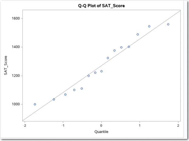
As you (hopefully) remember from Chapter 6, data values from a normal distribution would lie along the diagonal line. This plot does not show any strong deviations from a straight line and confirms the decision that you made by inspecting the histogram.
Nonparametric One-Sample Tests
If you do not feel that a t test is appropriate because of a non-normal distribution (especially if your sample size is relatively small), there is a nonparametric alternative called the Wilcoxon Signed Rank Test. To demonstrate how this test works, we will use a data set called Before_After that is included in the Create_Datasets.sas program. Remember, if you closed your SAS session, regardless of what platform you are using, you need to re-run the program to create all the WORK data sets.
The data set Before_After contains difference scores (variable name Difference) on a performance test, before and after several training sessions. Go ahead and run the t Tests task and inspect the tests of normality.
Figure 7.11: Tests of Normality for the Variable Difference
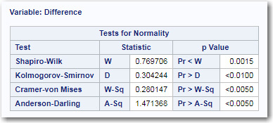
Because there are only 15 observations in this data set and all the tests for normality are significant, you proceed to look at the histogram.
Figure 7.12: Histogram and Box Plot

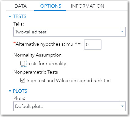
You decide that a t test is not appropriate and decide to run a nonparametric test. A nonparametric test does not require the assumption of normally distributed data. To run a Wilcoxon Signed Rank test, go to the OPTIONS tab and check the box under Nonparametric tests for Sign test and Wilcoxon signed rank test, as shown in Figure 7.13.
Figure 7.13: OPTIONS Tab for One-Sample T Tests
It’s time to run the procedure. Even though you selected an option for nonparametric tests, the task also runs a traditional t test as well. You can ignore that portion of output. For the curious, the p-value from the t test was .0431. Even though it is less than the traditional value of .05 for significance, you should ignore it. You want to scroll to the bottom of the results to see the p-value from the two nonparametric tests of interest, the Sign Test and the Wilcoxon Signed Rank Test.
Figure 7.14: Nonparametric Tests on the Difference Score
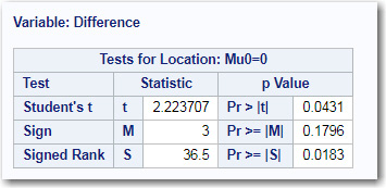
Of the two tests, the Signed Rank Test is usually the one you want to report. What follows is a description of both of these nonparametric tests.
The Sign Test simply looks to see whether the difference score is positive or negative. Under the null hypothesis, there should be an equal number of positive and negative values. The p-value for this test is based on a binomial probability. The p-value listed here is .1796 (that is, not significant). This test is most often used when the scores or differences can only be judged to be positive or negative, and a numerical value cannot be placed on the difference.
By comparison, the Signed Rank Test usually has more power to detect differences and is preferred if you have a measure of the differences. To conduct a Signed Rank Test, take the absolute value of all your differences (that is, ignore any minus signs) and rank them. If the difference is zero, ignore that value. Next determine the sign for each rank, based on the original values. If the null hypothesis is true, the positive and negative ranks should be about equal. If most of the higher ranks are of the same sign, you might have evidence to reject the null hypothesis. The probability is listed as .0183 (significant at the .05 level).
One of the advantages of running SAS Studio is the ease with which you can perform a large number of statistical tests. Yes, you still need to understand which tests to run and verify that the assumptions for those tests are satisfied. But once you have done this, getting your results is a few mouse clicks away.
1. Using the SAS data set Heart in the SASHELP library, use a one-way t test to determine if the mean weight of the population from which the sample was drawn is equal to 150 pounds. Include a test of normality and generate a histogram and box plot. Should you be concerned that the tests of normality reject the null hypothesis at the .05 level?
2. Using the data set Fish in the SASHELP library, test if the mean weight of Smelt (use a filter: Species = ‘Smelt’)) is equal to 10. Be sure to run both a parametric and nonparametric test for this analysis. How do the parametric and nonparametric tests compare? Would you reach the same conclusion using these tests?
3. Using the SAS data set Air in the SASHELP library, do the following:
a. List the first 10 observations from this data set.
b. Run summary statistics on the variable Air (number of flights per day in thousands). Include a histogram and box plot.
c. Run a parametric and nonparametric one-way t test to determine if the mean number of flights per day (in thousands) is significantly different from 285.
4. Run the short program below and then run a one-way t test to determine if the difference scores (Diff) come from a population whose mean is zero. In this program, the RAND function is generating uniform random numbers (numbers between 0 and 1 (all with equal likelihood). The DO loop generates 20 of these random numbers and outputs them to the Difference data set.
If you don’t like to type, this program and all the other programs associated with the exercises are included in the program Create_Datasets.sas.
data Difference;
call streaminit(13579);
do Subj = 1 to 20;
Diff = .6 - rand(‘uniform’);
output;
end;
run;
7. Rerun exercise 4, but change the value of 20 in the DO loop to 200. What do the tests for normality show? Is it OK to use a t test anyway? How did the p-value change?