Chapter 9: Comparing More Than Two Means (ANOVA)
Getting an Intuitive Feel for a One-Way ANOVA
Performing a One-Way Analysis of Variance
Performing More Diagnostic Plots
Performing a Nonparametric One-Way Test
When you want to compare means in a study where there are three or more groups, you cannot use multiple t tests. In the old days (even before my time!), if you had three groups (let’s call them A, B, and C), you might perform t tests between each pair of means (A versus B, A versus C, and B versus C). With four groups, the situation gets more complicated; you would need six t tests (A versus B, A versus C, A versus D, B versus C, B versus D, and C versus D). Even though no one does multiple t tests anymore, it is important to understand the underlying reason why this is not statistically sound.
Suppose you are comparing four groups and performing six t tests. Also, suppose that the null hypothesis is true, and all the means come from populations with equal means. If you perform each t test with α set at .05, there is a probability of .95 that you will make the correct decision—that is, to fail to reject the null hypothesis in each of the six tests. However, what is the probability that you will reject at least one of the six null hypotheses? To spare you the math, the answer is about .26 (or 26% if that is easier to think about). This is called an “experimentwise” type I error. Remember, a type I error is when you reject the null hypothesis (claim the samples come from populations with different means—“the drug works”) when you shouldn’t. So, instead of your chance of reporting a false positive result being .05, it is really .26.
To prevent this problem, statisticians came up with a single test, called analysis of variance (abbreviated ANOVA). The null hypothesis is that all the means come from populations with equal means; the alternative hypothesis is that there is at least one mean that is different from the others. You either reject or fail to reject the null hypothesis, and there is one p-value associated with the test. If you reject the null hypothesis, you can then investigate pairwise differences using methods that control the experimentwise type I error.
Getting an Intuitive Feel for a One-Way ANOVA
Before we get into the details of running and interpreting ANOVA tables, let’s get an intuitive feel for how this analysis works. Suppose you have three groups of subjects (A, B, and C) and you collected the following data:
|
Group |
A |
B |
C |
|
|
50 |
78 |
20 |
||
|
45 |
80 |
15 |
||
|
55 |
82 |
26 |
||
|
Means |
50 |
80 |
20 |
You see the means in groups A, B, and C are 50, 80, and 20 respectively. They seem pretty far apart. But, what does “far apart” mean? In this case, they are far apart compared to the scores within each group (which seem very close to the group mean). This might lead you to think that there is a significant difference between the groups.
In English, when there are more than two groups, proper grammar is to say “among”, not “between”. However, the terms “within” and “between” have been used to describe variances in ANOVA designs since they were first developed, and most textbooks have kept with these terms.
You can skip this next paragraph if you want—it describes how ANOVA works in more detail.
You can estimate the population variance by looking at the scores within a group or by using the group means to estimate the variance. If the null hypothesis were true (all the sample means come from populations with equal means), these two estimates of variance would be about the same and the ratio of the between-group variance to the within-group variance (called an F value) would be close to 1. If there were significant differences between the groups, the variance estimate computed by using the group means would be larger than the variance estimate computed by looking at the scores within a group. In this case, the F ratio would be greater than 1.
Performing a One-Way Analysis of Variance
We can use the data set called Reading (in the STATS library), containing data on reading speeds of males and females, as well as three different methods that might improve reading speeds of the test subjects, to demonstrate a one-way ANOVA.
Start by choosing the task One-Way ANOVA from the statistics Tasks / Linear Models task list. This brings up the following screen:
Figure 9.1: Selecting One-Way ANOVA from Linear Models List

To begin, double-click the One-Way ANOVA task tab.
Choose the data set Reading in the STATS library. This library was created when you ran the program Create_Datasets.sas. Choose Words_per_Minute as the Dependent variable and Method as the Categorical (independent) variable, as shown in Figure 9.2.
Figure 9.2: DATA Tab for One-Way ANOVA

Once you have completed the DATA screen, click the OPTIONS tab to see the following.
Figure 9.3: OPTIONS for One-Way ANOVA (Top Portion)

One of the assumptions for performing an analysis of variance is that the variances in each of the groups are equal. The Levene test is used to determine if this assumption is reasonable. If this test is significant (meaning the variances are not equal), you may choose to ignore it if the differences are not too large. (ANOVA is said to be robust to the assumption of equal variance, especially if the sample sizes are similar). If you want to account for unequal variances, click the box for Welch’s variance-weighted ANOVA.
Multiple comparisons are methods that you use in order to determine which pairs of means are significantly different. There are several choices for these tests. The default is Tukey, a popular choice. Later in this chapter, you will see another multiple comparison test called SNK (Student-Newman-Keuls). You probably want to leave the significance level at .05.
It’s time to run the procedure. Click the Run icon to produce the tables and graphs.
The first section of output displays class-level information. Don’t ignore this! Make sure that the number of levels is what you expected (data errors can cause the program to believe there are more levels than there are). Also, pay attention to the number of observations read and used. This is important because any missing values on either the dependent variable (Words_per_Minute) or categorical variable (Method) will result in that observation being omitted from the analysis. A large proportion of missing values in the analysis can lead to bias—subjects with missing values might be different in some way from subjects without missing values (that is, missing values might not be random).
Figure 9.4: Class-Level Information
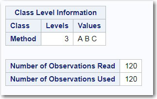
There are three levels for Method (A, B, and C) and there are no missing values (because the number of observations read is the same as the number of observations used). It’s time to look at your ANOVA table (Figure 9.5 below).
Figure 9.5: ANOVA Table

You can look at the F test and p-values in the ANOVA table, but you must remember that you also need to look at several other parts of the output to determine if the assumptions for the test are satisfied. You will see in the diagnostic tests that follow that the ANOVA assumptions were satisfied, so let’s go ahead and see what conclusions you can draw from the ANOVA table and the tables that follow.
Notice that the model has 2 degrees of freedom (because there were 3 levels of the independent variable, and the degrees of freedom is the number of groups minus 1). The mean squares for the model and error terms tell you the between-group variance and the within-group variance. The ratio of these two variances, the F value, is 20.84 with a corresponding p-value of less than .0001. A result such as this is often referred to as “highly significant.” Remember, the term “significant” means that the probability of falsely rejecting the null hypothesis is smaller than a pre-determined value. It doesn’t necessarily mean that the differences are significant in the common usage of the word, that is, important.
To graphically display the distribution of reading speed (Words_per_Minute) in the 3 groups, the one-way ANOVA task produces a box plot (Figure 9.6). The line in the center of the box represents the median, and the small diamond represents the mean. Notice that the means, as well as the medians, of the three groups are not very different. Why then were the results so highly significant? The reason is the large sample size (120). Large sample sizes give you high power to see even small differences.
Figure 9.6: Box Plot for Words_per_Minute by Method

Figure 9.7 shows the results for Levin’s test of homogeneity of variance. Here, the null hypothesis is that the variances are equal. Because the p-value is .9425, you do not reject the null hypothesis of equal variance.
Figure 9.7: Levene’s Test for Homogeneity of Variance

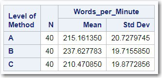
Figure 9.8 show the means and standard deviations for the three groups.
Figure 9.8: Means and Standard Deviations for the Three Groups
Because this is a one-way model, the least square means shown in Figure 9.9 (below) are equal to the means computed by adding up all the values within a group and dividing by the number of subjects in that group. In unbalanced models with more than one factor, this might not be the case.
Below the table showing the three means, you see p-values for all of the pairwise differences. Each of the three reading methods in the top table in the figure has what is labeled as the LSMEAN Number. In the table of p-values, the LSMEAN number is used to identify the groups. The intersection of any two groups displays the p-value for the difference. For example, group 1 (Method A) and group 2 (Method B) show a p-value of less than .0001. The p-value for the difference of Method A (1) and Method C (3) is .5514 (not significant).
Figure 9.9: Least Square Means
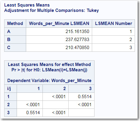
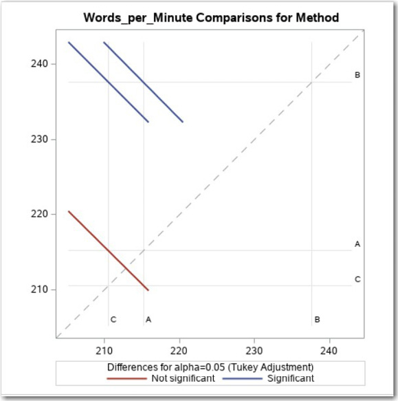
Figure 9.10 shows a very clever way to display pairwise differences. At the intersection of any two groups, you see a diagonal line representing a 95% confidence interval for the difference between the two group means. If the interval crosses the main diagonal line (that represents no difference), the two group means are not significantly different at the .05 level. To make this clearer, significant differences are seen in the two top diagonal lines representing C versus B and A versus B (they don’t cross the dotted line) and the diagonal line at the bottom left of the diagram representing C versus A, indicates a non-significant difference. By the way, the name diffogram is used to describe this method of displaying pairwise differences.
Figure 9.10: Pairwise Comparison of Means
All of the previous figures were generated by the choices that you made in the DATA and OPTIONS tabs. There is an alternative method of determining pairwise differences called the Student-Newman-Keuls (SNK) test (also referred to in some texts as just Newman-Keuls). The SNK test is similar to the Tukey test in that it shows group means and which pairs of means are different at the .05 level. The Tukey test has the advantage of computing p-values for each pair of means as well as a confidence interval for the differences. The SNK test can do neither of these two things but has a slightly higher power to detect differences.
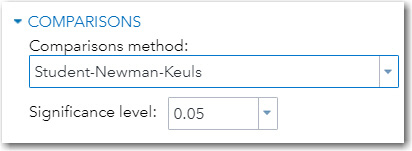
To request the SNK multiple comparison test, select Student-Newman-Keuls from the list under the Comparisons tab as shown in Figure 9.11
Figure 9.11: Requesting an SNK Multiple Comparison Test
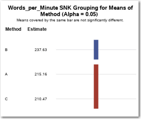
The SNK display (Figure 9.12) shows the three means in order from highest to lowest. Notice the bars on the right side of the output. Any two means that share the same bar are not significantly different at the .05 level. You can see here that the mean reading speed for group B is the highest, and it is significantly different from the mean of group A and from group C. Because groups A and C share a single bar, these two means (215.16 and 210.47) are not significantly different from each other.
Figure 9.12: Student-Newman-Keuls Pairwise Comparisons
Performing More Diagnostic Plots
Before we leave this section, let’s look at a few diagnostic plots that you can choose on the PLOTS menu. In the pull-down list below Diagnostic Plots, you can select either Panel of Plots or Individual plots. The Panel option shows all the plots on a single page—the Individual option shows each diagnostic plot on a separate page. In this example, you decided to see individual plots.
Figure 9.13: Requesting More Diagnostic Plots

The next several plots are intended to help you decide if the ANOVA assumptions were satisfied and to graphically show you information about the three means and the distribution of scores in each of the three groups.
The figures shown below were selected from a larger set of plots produced by the one-way ANOVA task.
The plot shown in Figure 9.14 shows the residuals (the differences between the mean of each group and each individual score in that group). There are actually two residual plots produced by the one-way task. One (shown here) displays the residuals as actual scores (words-per-minute, in this example). Another residual plot (not shown) displays the residuals as t scores (the number of standard deviations above or below the mean of the group). Both plots look very similar. You also see the predicted values (means of each group) shown on the X axis.
Figure 9.14: Residuals by Predicted Values
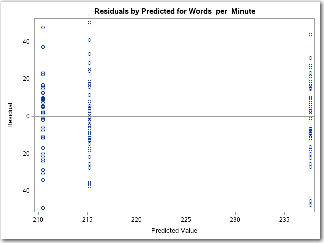
Notice that the residuals are spread out equally above and below the zero value for each of the three groups. This is another way to see that the variances in the three groups are not significantly different (as shown by the Levene Test).
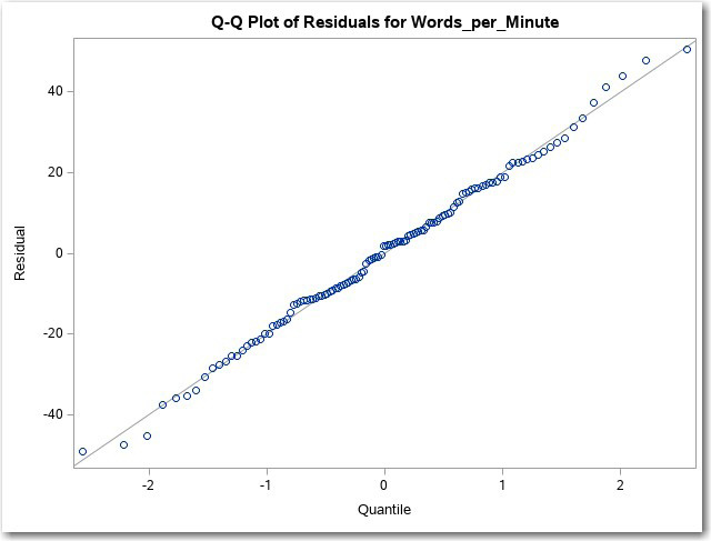
One of the assumptions for running a one-way ANOVA is that the errors (the residuals are estimates of these errors) are normally distributed. You have seen Q-Q plots earlier in this book, so you remember that data values that are normally distributed appear as a straight line on a Q-Q plot. The plot shown in Figure 9.15 shows small deviations from a straight line, but not enough to invalidate the analysis.
Figure 9.15: Q-Q Plot of the Residuals
Performing a Nonparametric One-Way Test
If you feel that the distribution assumptions are not satisfied by your data, another statistical task, Nonparametric One-Way ANOVA, provides a host of alternate tests. To demonstrate this, let’s go back to the SASHELP data set called Fish and compare the weights of three species of fish.
Start out by selecting Nonparametric One-Way ANOVA found under the Linear Models in the Tasks list (Figure 9.16).
Figure 9.16: Select Nonparametric One-Way ANOVA from the Linear Models Tab

Next, you want to create a filter to select three species: Bream, Roach, and Pike. The expression that you need to write is shown in Figure 9.17 below.
Figure 9.17: Creating a Filter for Three Species
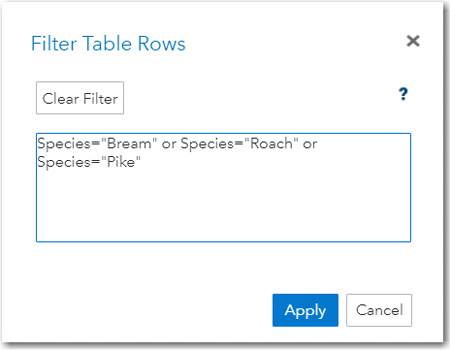
The names of the three species need to be placed in either single or double quotation marks because Species is a character variable. Once you apply this filter, only the three species will be used in the analysis.
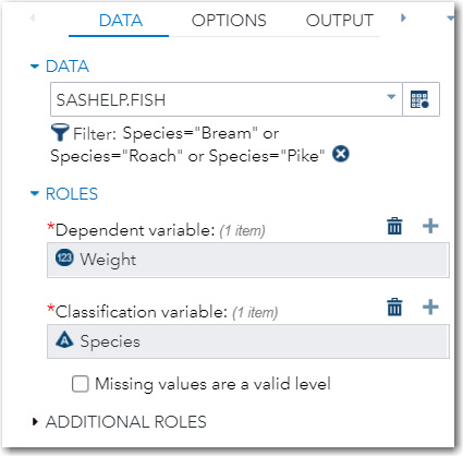
On the DATA Tab, select Weight as the Dependent variable and Species as the Classification variable (Figure 9.18).
Figure 9.18: Identifying the Dependent and Classification Variables
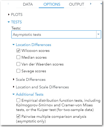
Next, click the OPTIONS tab. For this example, you are using all the default values except for a request for Pairwise multiple comparison analysis (asymptotic only).
Figure 9.19: Options for the Analysis
Now that you have entered your choices on the DATA and OPTIONS tabs, it’s time to run the task. The first part of the output is shown in Figure 9.20.
Figure 9.20: Results from the Wilcoxon Rank Sum Test
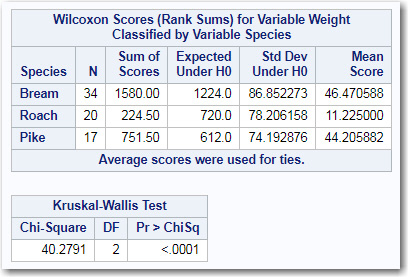
To perform the Wilcoxon Rank Sum Test, all the scores are sorted in order from the lowest score to the highest score. You then assign a rank to each score: the lowest score is rank 1, the next highest score is rank 2, and so on. If several scores are equal, the Wilcoxon test assigns the mean rank to each of the values (don’t worry about this detail for now). Along with the fish weights, you also know the species associated with each rank. There is a total of 71 fish weights (34 + 20 + 17), so the ranks range from 1 to 71. If the null hypothesis is that the fish are all about the same weight, you would expect the sum of ranks for each species to be about the same. You use this idea to form your null hypothesis. If one or more of the fish species has a very high or low sum of ranks, you might expect that there are differences in weight based on species.
The table above shows the sum of ranks for each of the fish species and the expected value if the null hypothesis is true. Notice that the sum of Scores for Roach (224.5) is much lower than the sums for Bream or Pike, making you suspect that Roach are typically lighter than either Bream or Pike. To decide whether you should reject the null hypothesis that all the three species have equal weights, you look at the p-value at the bottom of Figure 9.20. Because the p-value is shown as <.0001, you reject the null hypothesis and conclude that one or more pairs of means are significantly different. But, which pairs of fish species are different? We will answer that question in a minute.
The next part of the output shows box plots for each fish species. Box plots are appropriate for this display because you are conducting a nonparametric test.
Figure 9.21: Box plots for Each Species
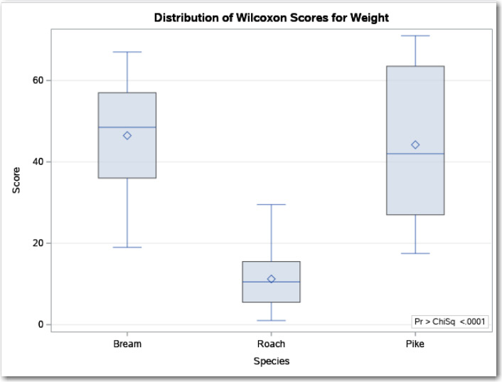
This plot shows that Roach seem to be lighter than either Bream or Pike. Just as you did a multiple comparison test in the ANOVA test (Tukey or SNK), there is an equivalent multiple comparison nonparametric test. Figure 9.22 shows significant differences between Bream versus Roach and Roach versus Pike. Bream and Pike are not statistically different (p = .8900).
Figure 9.22: Pairwise Comparisons

You have seen how to conduct a one-way analysis of variance as well as a Wilcoxon nonparametric test. You have also seen ways to determine if the two assumptions for a one-way ANOVA (normally distributed data and homogeneity of variance) are met.
1. List the first 10 observations from the High_School data set found in the STATS library (this was created when you ran the Create_Dataset.sas program in the download package). Conduct a one-way ANOVA comparing the variable Vocab_Score (a measure of vocabulary skill) by Grade (Freshman, Sophomore, Junior, and Senior). Be sure to run a Tukey multiple comparison test to determine which grades are different from each other (or none).
2. Repeat exercise 1, except this time, use the variable English_Grade as the dependent variable.
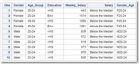
3. The data set Salary_Formatted in the STATS library contains variables Gender, Age_Group and Weekly_Salary. First, run the short program below to create a new variable (Gender_Age) that creates four combinations of the two variables Gender and Age_Group. (Hint: click on the new options icon and request a New Program.)
data Temp;
set Stats.Salary_Formatted;
length Gender_Age $ 6;
Gender_Age = Cats(Gender, Age_Group);
run;
The first 10 observations in the Temp data set should look like this:
Using the Temp data set, run a one-way analysis using Weekly_Salary as the dependent variable and Gender_Age as the categorical variable.
4. Using the data set Fish in the SASHELP library, compare the Width (not the Weight) of three species of fish; Perch, Roach, and Pike. Do this using both parametric and nonparametric methods. You will need to create a filter that reads:
Species=’Perch’ or Species=’Roach’ or Species=’Pike’
5. Using the data set Heart in the SASHELP library, run a nonparametric ANOVA using Cholesterol as your dependent variable and DeathCause as your classification variable. Include an option for multiple comparisons. Which, if any, of the causes of death had significant differences in cholesterol?
6. Using the data set Cars in the SASHELP library, compare the Horsepower for each Type of car. Use a filter (Type ne ‘Hybrid’) to eliminate hybrids because there are so few of them.
7. Using the data set Cars in the SASHELP library, compare the Weight of four-, six-, and eight-cylinder cars. Use a filter to restrict the variable Cylinders to values of 4, 6, or 8. Hint: the filter expression should read: Cylinders = 4 or Cylinders=6 or Cylinders=8. An interesting alternative is: Cylinders IN (4,6,8).