
i
i
i
i
i
i
i
i
206 8. Computer Vision in VR
(1) Pick one image as the reference
(2) Compute the homography H which maps the next
image in the sequence to the reference.
Use the four point correspondence described in Section 8.3.4,
or the RANSAC [5] algorithm can be used with a point
classification procedure to identify matched points [11, Ch. 4].
(3) Projectively align the second image with H
and blend in the non-overlapped part with the current
state of the panoramic image.
(4) Repeat the procedure from Step 2 until all the
images have been mapped and blended into the panorama.
Figure 8.18. The algorithm to assemble a panoramic mosaic from a number of indi-
vidual images.
8.3.6 Epipolar Geometry and the Fundamental Matrix
So far, we have really only considered scene reconstruction using one camera.
However, when a second, third or fourth camera becomes available to take
simultaneous pictures of the 3D world, a whole range of exciting opportu-
nities open up in VR. In particular, the realm of 3D reconstruction is very
important.
Again, the theory of scene reconstruction from multiple cameras is based
on rigorous maths. We will only briefly explore these ideas by introducing
epipolar geometry. This arises as a convenient way to describe the geometric
relationship between the projective views that occur between two cameras
looking at a scene in the 3D world from slightly different viewpoints. If the
geometric relationship between the cameras is known, one can get immediate
access to 3D information in the scene. If the geometric relationship between
the cameras is unknown, the images of test patterns allow the camera matrices
to be obtained from just the two images alone.
i
i
i
i
i
i
i
i
8.3. A Brief Look at Some Advanced Ideas in Computer Vision 207
All of the information that defines the relationship betw een the cameras
and allows for a vast amount of detail to be retrieved about the scene and
the cameras (e.g., 3D features if the relative positions and orientations of the
camerasisknown)isexpressedina4×4 matrix called the fundamental matrix.
Another 4 × 4 matrix called the essential matrix may be used at times when
one is dealing with totally calibrated cameras. The idea of epipolar geometry
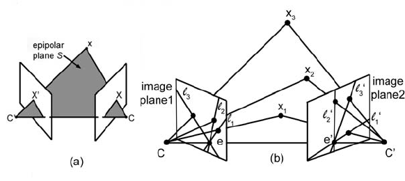
is illustrated in Figure 8.19(a), where the two camera centers C and C
and
the camera planes are illustrated.
Any point x in the world space projects onto points X and X
in the
image planes. Points x, C and C
define a plane S. The points on the image
plane where the line joining the camera centers intersect the image planes ar e
called the epipoles. The lines of intersection between S and the image planes
are called the epipolar lines, and it is fairly obvious that for different points x
there will be different epipolar lines, although the epipoles will only depend
on the camera centers and the location and orientation of the camera planes
(see Figure 8.19(b)).
Figure 8.19. (a) Point correspondences and epipolar relationships. (b) Variations of
epipolar lines. Point x
1
gives rise to epipolar lines l
1
and l
1
,pointx
2
to l
2
and l
2
etc.
Figure 8.20 shows how the epipolar lines fan out from the epipoles as x
moves around in world space; this is called the epipolar pencil.
Now, what we are looking for is a way to represent (parameterize) this
two-camera geometry so that information can be used in a number of inter-
esting ways. For example, we should be able to carry out range finding if we
know the camera geometry and the points X and X
on the image planes, or if
we know something about the world point, we can determine the geometric
relationship of the cameras.

i
i
i
i
i
i
i
i
208 8. Computer Vision in VR
Figure 8.20. Epipole and epipolar lines as they appear in the camera plane view.
In Section 8.3.3, all the important parametric details about a camera were
summed u p in the elements of the 3 × 3matrix,P.Itturnsoutthatanexact
analog exists for epipolar geometry; it is called the fundamental matrix F.
Analogous to the way P provided a mechanism of mapping points in 3D
space to points on the camera’s image plane, F provides a mapping, not from
P
3
to P
2
, but from one camera’s image of the world point x to the epipolar
line lying in the image plane of the other camera (see Figure 8.21).
This immediately gives a clue as to how to use a two-camera set-up to
achieve range finding of points in world space if we know F :
Figure 8.21. A point projected onto the image plane of camera 1 is mapped to some
point lying on the epipolar line in the image plane of camera 2 by the fundamental
matrix F.
i
i
i
i
i
i
i
i
8.3. A Brief Look at Some Advanced Ideas in Computer Vision 209
Take the projected image of a scene with two cameras. Use image
processing software to identify key points in the picture from im-
age 1. Apply F to these points in turn to find the epipolar lines
in image 2 for each of these points. Now use the image process-
ing software to search along the epipolar lines and identify the
same point. With the location in both projections known and
the locations and orientations of t he cameras known, it is sim-
ply down to a bit of coordinate geometry to obtain the world
coordinate of the key points.
But there is more: if we can range find, we can do some very interesting
things in a virtual world. For example, we can have virtual elements in a
scene appear to interact with real elements in a scene viewed from two video
cameras. The virtual objects can appear to move in front of or behind the real
objects.
Let’s return to the question of how to specify and determine F and how
to apply it. As usual, we need to do a bit of mathematics, but before we do,
let us recap some vector rules that we will need to apply:
• Rule 1: The cross product of a vector with itself is equal to zero. For
example, X
3
×X
3
= 0.
• Rule 2: The dot product of a vector with itself can be rewritten as
the transpose of the vector matrix multiplied by itself. For example,
X
3
· X
3
= X
T
3
X
3
.
• Rule 3: Extending Rule 1, we can write X
3
· (X
3
× X
3
) = 0.
• Rule 4: This is not so much of a rule as an observation. The cross
product of a vector with another vector that has been transformed by a
matrix can be rewritten as a vector transformed by a different matrix.
For example, X
3
× T X
3
= MX
3
.
Remembering these four rules and using Figure 8.22 as a guide, let X
3
=
[x, y, z, w]
T
represent the coordinates in P
3
of the image of a point in the first
camera. Using the same notation, the image of that same point in the second
camera is at X
3
= [x
, y
, z
, w]
T
, also in world coordinates. These positions
are with reference to the world coordinate systems of each camera. After
projection onto the image planes, these points are at X = [X , Y , W ]
T
and
X
= [X
, Y
, W ]
T
, respectively, and these P
2
coordinates are again relative
to their respective projection planes. (Note: X
3
and X represent the same
i
i
i
i
i
i
i
i
210 8. Computer Vision in VR
point, but X
3
is relative to the 3D world coordinate system with its origin at
C,whereasX is a 2D coordinate relative to an origin at the bottom left corner
of the image plane for camera 1.)
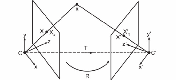
Figure 8.22. Two-camera geometry; the second camera is positioned relative to the
first with a rotation R followed by a translation T .
Now, assuming that the properties of the cameras are exactly the same,
apply the necessary translation and rota tion to the first camera so that it lies
at the same location and points in the same direction as the second camera.
Then X
3
will have been moved to X
3
, and thus
X
3
= T X
3
,
where T is a transformation matrix that represents the rotation and transla-
tion of the frame of origin of camera 1 to that of camera 2.
Now if we consider Rule 3, which stated
X
3
· (X
3
× X
3
) = 0,
then we can replace one of the X
3
terms with TX
3
. That is,
X
3
· (X
3
× T X
3
) = 0.
Utilizing R ule 2, we can rewrite this equation as
X
T
3
(X
3
× T X
3
) = 0,
and bringing in Rule 4, we can simplify this expression to
X
T
3
MX
3
= 0, (8.8)
..................Content has been hidden....................
You can't read the all page of ebook, please click here login for view all page.