
i
i
i
i
i
i
i
i
8.3. A Brief Look at Some Advanced Ideas in Computer Vision 201
equivalent inhomogeneous formulation. Of course, there still is the little
matter of solving the linear system, but the DLT algorithm offers a solution
through singular value decomposition (SVD). For details of the SVD step,
which is a general and very useful technique in linear algebra, see [12].
Singular value decomposition factoriz es a matrix (which does not have to
be square) into the form A = LDV
T
,whereL and V are orthogonal matrices
(i.e., V
T
V = I) and D is a diagonal. (D is normally chosen to be square, but
it does not have to be.) So, for example, if A is 10 ×8thenL is 10 ×10, D is
10 ×8 and V
T
is 10 × 10. It is typical to arrange the elements in the matrix
D so that the largest diagonal coefficient is in the first row, the second largest
in the second row etc.
For example, the SVD of
⎡
⎣
11
01
10
⎤
⎦
=
⎡
⎢
⎣
√
6
3
0
√
3
3
√
6
6
−
√
6
6
−
√
3
3
√
6
6
√
2
2
−
√
3
3
⎤
⎥
⎦
⎡
⎣
√
30
01
10
⎤
⎦
√
2
2
√
2
2
√
2
2
−
√
2
2
.
There are two steps in the basic direct linear transform algorithm. They
are summarized in Figure 8.12. The DLT algorithm is a great starting point
for obtaining a transformation that will correct for a perspective projection,
but it also lies at the heart of more sophisticated estimation algorithms for
solving a number of other computer vision problems.
We have seen that the properties of any camera can be concisely specified
by the camera matrix. So we ask, is it possible to obtain the camera matrix
itself by examining correspondences from points (not necessarily lying on a
plane) in 3D space to points on the image plane? That is, we are examining
correspondences from P
3
to P
2
.
Of course the answer is yes. In the case we have just discussed, H was a
3 × 3 matrix whereas P is dimensioned 3 × 4. However, it is inevitable that
the estimation technique will have to be used to obtain the coefficients of P.
Furthermore, the only differences between the expressions for the coefficients
of H (Equation (8.6)) and those of P arise because the points in P
3
have four
coordinates, and as such we will have a m atrix of size 2n × 12. Thus the
analog of Equation (8.6) can be expressed as Ap = 0, and the requirement
for the estimation to work is n ≥ 6. (That is, 6 corresponding pairs with 12
coefficients and 11 degrees of freedom.)

i
i
i
i
i
i
i
i
202 8. Computer Vision in VR
(1) From each point mapping, compute the corresponding
two rows in the matrix A in Ah = 0
and assemble the full 2n × 9 A matrix.
Note that h contains all the coefficients in H
written an a vector.
(2) Compute the SVD of A. If the SVD r esults in
A = LDV
T
, the elements in H are given by
the last column in V , i.e., the last row of V
T
.
(e.g., if the A matrix is dimensioned (64 × 9) then L is
(64 × 64), D is (64 × 9) and L is (9 ×9) )
Figure 8.12. Obtaining the matrix H using the DLT algorithm with n point cor-
respondences. In practice, the DLT algorithm goes throu gh a pre-processing step
of normalization, which helps to reduce numerical problems in obtaining the SVD
(see [7, pp. 88–93]).
In this case, if we express the correspondence as (x
i
, y
i
, z
i
, w
i
) → (X
i
, Y
i
, W
i
)
from P
3
to P
2
and let
x
T
i
= [x
i
, y
i
, z
i
, w
i
],
p0
i
= [p
00
, p
01
, p
02
, p
03
]
T
,
p1
i
= [p
10
, p
11
, p
12
, p
13
]
T
,
p2
i
= [p
20
, p
21
, p
22
, p
23
]
T
,
then the 12 coefficients of P are obtained by solving
W
i
x
T
i
0 −X
i
x
T
i
0 −W
i
x
T
i
Y
i
x
T
i
⎡
⎣
p0
i
p1
i
p2
i
⎤
⎦
= 0. (8.7)
The DLT algorithm is equally applicable to the problem of obtaining
P given a set of n ≥ 6 point correspondences from points in world space
(x
i
, y
i
, z
i
, w
i
) to points on the image plane, (X
i
, Y
i
, W
i
). However, there are
i
i
i
i
i
i
i
i
8.3. A Brief Look at Some Advanced Ideas in Computer Vision 203
some difficulties in practice, as there are in most numerical methods, that
require some refinement of the solution algorithm. For example, the lim-
ited numerical accuracy to which computers work implies that some form of
scaling (called normalization) of the input data is required before the DLT al-
gorithm is applied. A commensurate de-normalization has also to be applied
to the result.
We refer the interested reader to [7, pp. 88–93] for full details of a robust
and successful algorithm, or to the use of computer vision software libraries
such as that discussed in Section 8.4.
8.3.5 Reconstructing Scenes from Images
One of the most interesting applications for computer vision algorithms in
VR is the ability to reconstruct scenes. We shall see (in Section 8.3.7) that
if you have more than one view of a scene, some very accurate 3D informa-
tion can be r ecovered. If you only have a single view, the opportunities are
more limited, but by making some assumptions about parallel lines, vanish-
ing points and the angles between structures in the scene (e.g., known to be
orthogonal) some useful 3D data can be extracted.
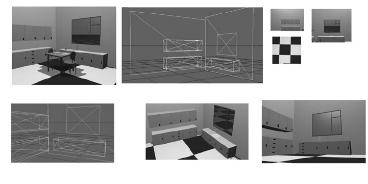
An example of this is illustrated in Figure 8.13. Figure 8.13(a) is a photo-
graph of a room. Figure 8.13(b) is a view of a 3D model mesh reconstructed
from the scene. (Note: some of the structures have been simplified because
(a)
(b)
(c)
(d) (e)
(f)
Figure 8.13. Reconstructing a 3D scene from images.

i
i
i
i
i
i
i
i
204 8. Computer Vision in VR
simple assumptions regarding vanishing points and the line a t infinity have
to be accepted.) Figure 8.13(c) shows image maps recovered from the pic-
ture and corrected for perspective. Figure 8.13(d) is a different view of the
mesh model. Figure 8.13(e) is a 3D rendering of the mesh model with image
maps applied to surfaces. Figure 8.13(f ) shows the scene rendered from a
low-down viewpoint. (Note: some minor user modifications were required to
fix the mesh and maps after acquisition.) The details of the algorithms that
achieve these results are simply variants of the DLT algorithm we examined
in Section 8.3.4.
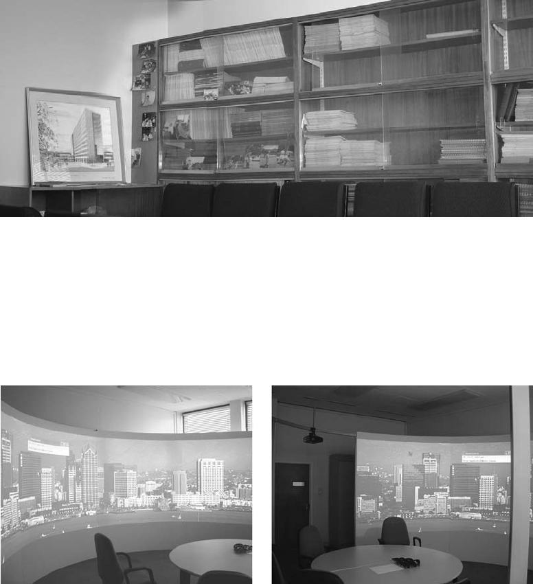
In an extension to this theory, it is also possible to match up several ad-
joining images taken by rotating a camera, as illustrated in Figure 8.14. For
example, the three images in Figure 8.15 can be combined to give the single
image shown in Figure 8.16. This is particularly useful in situations where
you have a wide display area and need to collate images to give a panoramic
view (see Figure 8.17). A simple four-step algorithm that will assemble a
single panoramic composite image from a number of images is given in Fig-
ure 8.18.
Figure 8.14. A homography maps the image planes of each photograph to a reference
frame.
Figure 8.15. Three single photos used to form a mosaic for part of a room environ-
ment.
i
i
i
i
i
i
i
i
8.3. A Brief Look at Some Advanced Ideas in Computer Vision 205
Figure 8.16. The composite image.
Figure 8.17. A composite image used in an immersive VR environment. In this
particular example, the image has been mapped to a cylindrical screen.
..................Content has been hidden....................
You can't read the all page of ebook, please click here login for view all page.