
i
i
i
i
i
i
i
i
262 11. Navigation and Movement in VR
or equivalently (to speed up its calculation),
p(
) = ((K
3
+ K
2
) + K
1
) + K
0
.
The unknown vector constants K
0
, K
1
, K
2
and K
3
, as well as the parameter ,
have to be determined. To do this, we initially impose four conditions on
Equation (11.1):
1. The spline passes through the point P
i
at the start of the curve. At this
point, = 0.
2. The spline passes through the point P
i+1
at the end of the curve. At
this point, = 1
3. The derivative of the spline at P
i
is given. That is P
i
.
4. The derivative of the spline at P
i+1
is given. That is P
i+1
.
The parameter
in the equations for the spline is related to the distance
traveled along a given section of the curve. This is shown in Figure 11.2. In
addition, in order to determine the vector constants, we only utilize a segment
of the spline available.
Obviously, in 3D space, there are three components (x, y, z) to any vector
position p, and these conditions apply to each of these components. For
example, to obtain the x-component we need to consider the values x
i
, x
i+1
,
x
i
, x
i+1
.
In addition, differentiating Equation (11.1) with respect to gives us a
standard equation by which we can specify p
( ):
p
( ) = 3K
3
2
+ 2K
2
+ K
1
. (11.2)
Thus,inEquation(11.1),ifwesubstitute
with 0 to represent p(x
i
) and
with 1 to represent p(x
i+1
), and in Equation (11.2) if we substitute with
0torepresentp
(x
i
) and with 1 to represent p
(x
i+1
), we will have four
simultaneous equations which can be used to solve for the x-component of
the vector constants K
0
, K
1
, K
2
, K
3
. Written in matrix form, these are
⎡
⎢
⎢
⎣
0001
1111
0010
3210
⎤
⎥
⎥
⎦
⎡
⎢
⎢
⎣
K
3
x
K
2
x
K
1
x
K
0
x
⎤
⎥
⎥
⎦
=
⎡
⎢
⎢
⎣
x
i
x
i+1
x
i
x
i+1
⎤
⎥
⎥
⎦
.

i
i
i
i
i
i
i
i
11.2. Moving and Rotating in 3D 263
On solution, the following expressions are obtained:
K
3
x
= 2x
i
− 2x
i+1
+ x
i
+ x
i+1
,
K
2
x
= −3x
i
+ 3x
i+1
− 2x
i
− x
i+1
,
K
1
x
= x
i
,
K
0
x
= x
i+1
.
However, as you can see, determination of the vector constants is depen-
dent on finding the gradient of the spline (or its derivative) at the two control
points, P
i
and P
i+1
. Remember that we can only define a spline using a min-
imum of four values. Thus we can use the knowledge we have of the other
two points (P
i−1
and P
i+2
) on the spline in order to estimate the derivative
at P
i
and P
i+1
. We do this using finite differences, where x
i
=
x
i+1
−x
i−1
2
and
x
i+1
=
x
i+2
−x
i
2
. That is, we are really finding the gradient of the spline at
these two points.
This results in the following sequence of equations:
K
3
x
= −
1
2
x
i−1
+
3
2
x
i
−
3
2
x
i+1
+
1
2
x
i+2
, (11.3)
K
2
x
= x
i−1
−
5
2
x
i
+ 2x
i+1
−
1
2
x
i+2
, (11.4)
K
1
x
= −
1
2
x
i−1
+
3
2
x
i+1
, (11.5)
K
0
x
= x
i
. (11.6)
Similar expressions may be written for the y- and z-components of the K
terms, and thus the constant vectors K
c
become
K
c
=
⎡
⎣
K
c
x
K
c
y
K
c
z
⎤
⎦
,
for c = 0, 1, 2, 3.
At this stage, we need to draw a distinction about how we intend to use
our spline. When we are animating camera movement, for example, P
i−1
to
P
i+2
are all predetermined positions of the camera. That is, they are key posi-
tions. Then we can simply interpolate between these predetermined positions
in order to estimate how the camera moves so that the transition will appear
smooth, with no sudden changes of direction. We can do this by using Equa-
tion (11.1) to determine any position p at time t along the spline. Of course,

i
i
i
i
i
i
i
i
264 11. Navigation and Movement in VR
in order to use this equation, we need to insert a value for . Assuming that
an object following the spline path is getting its known loca tions (the P
i
)at
equal time intervals t, we can parameterize the curve by time and obtain
from
=
t − t
−2
t
.
This arises because the spline has been determined using four control
positions. In Figure 11.2, these contr ol points are P
i−1
, P
i
, P
i+1
and P
i+2
.
To determine the constant vectors, we set
= 0atP
i
. If we wished to
interpolate between control points P
i+1
and P
i+2
,wewouldusevaluesof
in the range 1 < < 2.
Of course, as we mentioned earlier, spline interpolation is only useful
when we have predetermined key positions. Extrapolation is required when
there is no knowledge of future movement. Take for example our flight sim-
ulator, where we obtain information about position from external hardware
every second. However, suppose we must render our frames every hundredth
of a second. Assuming that P
i+2
is the last known position obtained from the
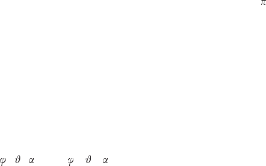
Figure 11.2. A spline segment used for interpolation and extrapolation. The
parameterτ lies in the interval [0, −1] between the points P
i−1
and P
i
,andp is a
position on the curve at any time t > t
0
.
i
i
i
i
i
i
i
i
11.2. Moving and Rotating in 3D 265
hardware, our software needs to extrapolate the position of our aircraft every
one hundredth of a second until the next position, P
i+3
, is available from the
hardware.
Again, we may use Equation (11.1) to determine the position p at any
time greater than t. Thus we try to predict how the spline will behave up
until our system is updated with the actual position. This may or may not
be the same as our extrapolated position. Typically, parameterization by time
and extrapolation can lead to a small error in predicted position. For example,
the point labeled P
actual
in Figure 11.2 is the actual position of the next point
along the true path, but it lies slightly off the predicted curve.
So we need to recalculate the equation of the spline based on this current
actual position and its previous three actual positions. Thus, P
i
becomes P
i−1
and so on. Using the four new control positions, we recompute the spline,
and this new spline will then be used to predict the next position at a given
time slice. And so the procedure continues.
It is also worth noting at this stage that whilst spline extrapolation is not
without error, linear extrapolation is usually much more error-prone. For the
example in Figure 11.2, if linear extrapolation of the positions P
i+1
and P
i+2
is used to predict the new position at time t, the associated positional error is
much greater than with spline interpolation.
11.2.2 Rotating Smoothly
In this section, we turn our attention to interpolating angles of orientation.
Angles cannot be interpolated in the same way as position coordinates are in-
terpolated. For one thing they are periodic in the interval [0, −2
]. It is now
generally agreed that the best way to obtain smooth angular interpolation is
by using quaternions. Appendix A provides the background on quaternions.
It gives algorithms for converting between Euler angles, quaternions and rota-
tion matrices, and defines the function specifically for solving the problem of
orientation tweening; that is, the slerp() function. It also dem onstrates how to
calculate the transformation matrix used to set the orientation for an object or
direction of view T
a
k
at time t
k
, obtained by interpolation of the orientations
at times t
l
and t
m
.
T
a
k
cannot be obtained by directly interpolating the matrices express-
ing the orientation at times t
l
and t
m
(see Section A.2). At times t
l
and t
m
,
the matrices T
a
l
and T
a
m
are actually determined from the known values
of (
l
,
l
,
l
) and (
m
,
m
,
m
) respectively. Therefore, whilst it may not be
possible to interpolate matrices, it is possible to interpolate a quaternion asso-

i
i
i
i
i
i
i
i
266 11. Navigation and Movement in VR
ciated with a rotation matrix using the slerp() function in the following three
steps:
1. Given an orientation that has been expressed in Euler angles at two
time points, l and m, calculate equivalent quaternions q
l
and q
m
, using
the algorithm given in section A.2.1.
2. Interpolate a quaternion q
k
that expresses the orientation at time t
k
using:
=
t
k
− t
l
t
m
− t
l
;
= cos
−1
q
l
· q
l
;
q
k
=
sin(1 − )
sin
q
l
+
sin
sin
q
m
.
See Appendix A for details.
3. Us e the expressions from Section A.2.2 to obtain T
a
k
given the quater-
nion q
k
.
And there we have it: T
a
k
is a matrix representing the orientation at time
t
k
so that the orientation of any object or the viewpoint changes smoothly
during the interval t
l
to t
m
.
11.3 Robotic Motion
Consider the following scenario:
You are wearing a haptic feedback glove and a head-mounted
stereoscopic display (HMD). The headset and the glove con-
tain sensors that feed their position and orientation into a VR
simulator with computer-generated characters. It should be pos-
sible for you to reach forward and shake hands with one of the
synthetic characters or take the synthetic dog for a walk. The
stereoscopic HMD should confuse y our eyes into believing the
character is standing in front of you; the haptic glove should give
you the illusion of a firm handshake.
3
Now for the movement
3
We haven’t seen this actually done yet, but all the hardware components to achieve it are
already commercially available.
..................Content has been hidden....................
You can't read the all page of ebook, please click here login for view all page.