

i
i
i
i
i
i
i
i
11.4. Inverse Kinematics 277
Star t with the linkage configuration defined by the set of angles:
θ
1
, θ
2
, θ
3
...θ
n
(which we will write as Θ), and endpoint located at P,
i.e., at coordinate (x, y).
Apply the steps below to move the endpoint towards its goal
at P
g
(i.e., at :(x
g
, y
g
))
Step 1:
Calculate the incremental step ΔX = P
g
− P
Step 2:
Calculate J(θ
1
, θ
2
, θ
3
, ...θ
n
)
(use the current values of θ
1
etc.)
Step 3:
Find the inverse of J, which we will call J
−
J
−
= J
T
(JJ
T
)
−1
(if J is a 2 × n matrix, J
−
is a n × 2matrix)
Step 4:
Test for a valid convergence of the iteration:
if (I − JJ
−
)ΔX > ε then the step towards the
goal (the ΔX) is too large, so set ΔX =
ΔX
2
and repeat Step 4 until the norm is less than ε.
If the inequality cannot be satisfied after a certain number
of steps then it is likely that the goal cannot be reached and
the IK calculations should be terminated
(Thisstepisdiscussedinmoredetailinthetext)
Step 5:
Calculate updated values for the parameters θ
1
etc.
Θ = Θ + J
−
ΔX
Θ is the vector of angles for each link [θ
1
, θ
2
, ...]
T
Step 6:
Calculate the new state of the articulation from θ
1
, θ
2
etc.
Check the endpoint P
4
to see if is close enough to the goal.
It is likely that ΔX will have been reduced by Step 4
and thus the endpoint will be somewhat short of the goal.
In this case, go back and repeat the procedure from Step 1.
Otherwise, we have succeeded in moving P
4
to the goal point P
g
Figure 11.8. I t erative algorithm for solving the IK problem to determine the orienta-
tion of an articulated linkage in terms of a number of parameters θ
i
given the goal of
moving the end of the articulation from its current position P towards X
g
.

i
i
i
i
i
i
i
i
278 11. Navigation and Movement in VR
vector X − J( ) is smaller than a specified threshold:
X − J( ) < .
If we substitute for
and call J
−
the generalized inverse of J,thenin
matrix form,
X − JJ
−
X < ,
or simplifying we have
(I − JJ
−
) X < ,
where I is the identity matrix such that I(
X) = X.
We use this criterion to determine a X that satisfies the condition on
the norm. We also use this to determine whether the iteration can proceed,
or whether we must accept that the goal cannot be reached. A simple test on
the magnitude of
X will suffice: when it is less than a given threshold, then
either the goal has been reached or it is so small that the end will never get
there.
Equations for a General Two-Dimensional Articulated Linkage
To extend the solution technique to n links in 2D, we essentially use the same
algorithm, but the expressions for (x, y) and the Jacobian terms
∂x
∂
i
become
x =
n
i=1
l
i
cos(
i
j=i
j
),
y =
n
i=1
l
i
sin(
i
j=i
j
),
∂x
∂
k
= −
n
i=k
l
i
sin(
i
j=1
j
),
∂y
∂
k
=
n
i=k
l
i
cos(
i
j=1
j
);
k = 1, ···, n .
11.4.3 Solving the IK Problem in Three Dimensions
All the steps in the solution procedure presented in Figure 11.8 are equally
applicable to the 3D IK problem. Calculation of generalized inverse, iteration
i
i
i
i
i
i
i
i
11.4. Inverse Kinematics 279
towards a goal for the end of the articulation and the termination criteria are
all the same. Where the 2D and 3D IK problems differ is in the specification
of the orientation of the links, the determination of the Jacobian and the
equations that tell us how to calculate the location of the joints between links.
Although the change from 2D to 3D involves an increase of only one
dimension, the complexity of the calculations increases to such an extent
that we cannot normally determine the coefficients of the Jacobian by differ-
entiation of analytic expressions. Instead, one extends t he idea of iteration
to write expressions which relate infinitesimal changes in linkage orienta-
tion to infinitesimal changes in the position of the end effector. By making
small changes and iterating to war ds a solution, it becomes possible to calcu-
late the Jacobian coefficients under the assumptions that the order of rotat-
ional transformation does not matter, and that in the coefficients, sin
→ 1
and cos → 1. We will not consider the details here; they can be found
in [1]. Instead, we will move on to look at a very simple algorithm for IK in
3D.
A Simple IK Algorithm for Use in Real Time
The Jacobian IK algorithm is well defined analytically and can be rigorously
analyzed and investig ated, but in practice it can sometimes fail to converge. In
fact, all iterative algorithms can sometimes fail to converge. However, when
the Jacobian method fails to converge, it goes wrong very obviously. It does
not just grind to a halt; it goes way over the top! Hence, for our VR work,
we need a simple algorithm that can be applied in real time and is stable and
robust.
A heuristic algorithm called the cyclic coordinate descent (CCD) method [3]
works well in practice. It is simple to implement and quick enough to use in
real time even though it doesn’t always give an optimal solution. It consists of
the five steps given in F i gure 11.9.
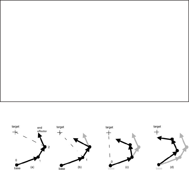
The algorithm is best explained with reference to the example given
in Figures 11.10 and 11.11. The steps are labeled (a) to (h), where (a) is
the starting configuration. A line joining pivot point 2 to the target shows
how the last link in the chain should be rotated about an axis perpendicular
to the plane in which links 1 and 2 lie. After this rotation, the linkage will
lie in the position shown in (b). Next, the linkage is rotated about point 1 so
that the end effector lies on the line joining point 1 to the target point. This
results in configuration (c), at which time a rotation about the base at point 0
is made to give configuration (d). This completes round 1 of the animation.
Figure 11.11 configuration (e) is the same as Figure 11.11(d), and a pivot
i
i
i
i
i
i
i
i
280 11. Navigation and Movement in VR
Step 1:
Star t with the last link in the chain (at the end effector).
Step 2:
Set a loop counter to zero. Set the max loop count to some upper limit.
Step 3:
Rotate this link so that it points towards the target. Choose
an axis of rotation that is perpendicular to the plane defined
by two of the linkages meeting at the point of rotation.
Do not violate any angle restrictions.
Step 4:
Move down the chain (away from the end effector) and go back to Step 2.
Step 5:
When the base is reached, determine whether the target has
been reached or the loop limit is exceeded. If so, exit;
if not, increment the loop counter and repeat from Step 2.
Figure 11.9. The cyclic coordinate descent iterative algorithm for manipulating an IK
chain into position. It works equally well in two or three dimensions.
Figure 11.10. The cyclic coordinate descent algorithm. Iteration round 1 (loop
count=1). The original position of the linkage is shown in light grey.
at point 2 is made to give configuration (f). Further pivots about point 1
result in configuration (g). F inally, a pivot about point 0 leads to config-
uration (h), by which time the end effector has reached the target and the
iteration stops.
Of course, there are many other configurations that would satisfy the goal
of the end effector touching the target, but the configuration achieved with
the CCD algorithm is the one that feels natural to the human observer. It is
also possible that in certain circumstances, the end effector may never reach

i
i
i
i
i
i
i
i
11.5. Summary 281
Figure 11.11. The cyclic coordinate descent algorithm. Iteration round 2 (loop
count=2) completes the cycle because the end effector had reached the target.
the goal, but this can be detected by the loop count limit being exceeded.
Typically, for real-time work, the loop count should never go beyond five.
The Jacobian method has the advantage of responding to pushes and pulls
on the end effector in a more natural way. The CCD method tends to move
the link closest to the end effector. This is not surprising when y ou look at
the algorithm, because if a rotation of the last linkage reaches the target, the
algorithm can stop. When using these methods interactively, there are notice-
able differences in response; the CCD behaves more like a loosely connected
chain linkage whilst the Jacobian approach gives a configuration more like
one would imagine from a flexible elastic rod. In practical work, the CCD
approach is easy to implement and quite stable, and so is our preferred way
of using IK in real-time interactive applications for VR.
11.5 Summary
This chapter looked at the theory underlying two main aspects of movement
in VR, rigid motion and inverse kinematics (IK). Rigid motion is performed
by using some form of interpolation or extrapolation, either linear, quadratic,
or cubic in the form of a 3D parametric spline. Interpolation is also important
in obtaining smooth rotation and changes of direction. In this case, the most
popular approach is to use quaternion notation. That was explained together
with details of how to convert back and forward from the more intuitive Euler
angles and apply it in simulating hierarchical motion.
IK is fundamentally important in determining how robots, human avatars
and articulated linkages move when external forces are applied at a few of
their joints. We introduced two algorithms that are often used to express
IK behavior in VR systems, especially when they must operate in real time.
..................Content has been hidden....................
You can't read the all page of ebook, please click here login for view all page.