3
Fuzzy Numbers and Their Arithmetic
Fuzzy numbers are a mathematical formulation of vague statements about real numbers. For example, a statement expressing that a number is approximately 2 is modeled by a fuzzy number. Fuzzy numbers are of great importance in fuzzy systems and toward the end of this chapter, we are going to discuss how we can construct fuzzy numbers from real‐world data, and how these numbers can be used.
3.1 Fuzzy Numbers
Fuzzy (real) numbers are a special kind of fuzzy sets that have been introduced by Zadeh [311].
Clearly, every fuzzy number is a convex fuzzy set since all α‐cuts are closed intervals. Also, the core of a fuzzy number ![]() should be a singleton, and we will denote its only element by
should be a singleton, and we will denote its only element by ![]() . Fuzzy numbers can be either positive or negative:
. Fuzzy numbers can be either positive or negative:
A special case of fuzzy real numbers are the discrete fuzzy numbers. A fuzzy subset of ![]() is a discrete fuzzy number if its support is finite. If
is a discrete fuzzy number if its support is finite. If ![]() is a discrete fuzzy number and
is a discrete fuzzy number and ![]() , then there is an
, then there is an ![]() such that
such that ![]() . In the rest of this section, we present the various types of nondiscrete fuzzy numbers, and we mostly follow the categorization and the definitions presented in [159].
. In the rest of this section, we present the various types of nondiscrete fuzzy numbers, and we mostly follow the categorization and the definitions presented in [159].
If the universe on which a fuzzy set is defined is the set ![]() of complex numbers, then fuzzy sets are called fuzzy complex numbers [40]. The α‐cuts of a fuzzy complex number
of complex numbers, then fuzzy sets are called fuzzy complex numbers [40]. The α‐cuts of a fuzzy complex number ![]() are
are
where ![]() and, when
and, when ![]() , then we separately specify
, then we separately specify
Although the theory of fuzzy complex numbers is quite interesting, we are not going to present its details in this book.
3.1.1 Triangular Fuzzy Numbers
A triangular fuzzy number is a fuzzy set whose graph is a triangle. Usually, one specifies such a fuzzy number using the notation ![]() , where
, where ![]() is the only element of the core of the fuzzy number and corresponds to the
is the only element of the core of the fuzzy number and corresponds to the ![]() ‐coordinate of the point that lies at the intersection of the altitude and the base,
‐coordinate of the point that lies at the intersection of the altitude and the base, ![]() is the length of the line segment from
is the length of the line segment from ![]() to the vertex that lies to the left of it, and
to the vertex that lies to the left of it, and ![]() is the length of the line segment from
is the length of the line segment from ![]() to the vertex that lies to the right of it. Figure 3.1 depicts a triangular fuzzy number and its “coordinates.” A triple
to the vertex that lies to the right of it. Figure 3.1 depicts a triangular fuzzy number and its “coordinates.” A triple ![]() defines a fuzzy number that is characterized by the following membership function:
defines a fuzzy number that is characterized by the following membership function:


Figure 3.1 A triangular fuzzy number.
Alternatively, this membership function can be expressed as follows:
In fact, this alternative formulation can be easily used to draw any triangular fuzzy number.
3.1.2 Trapezoidal Fuzzy Numbers
Trapezoidal fuzzy numbers are, of course, fuzzy sets but since their core contains more than one element, they cannot be classified as fuzzy numbers. However, it is absolutely reasonable to view these fuzzy sets as fuzzy intervals. On the other hand, it is a fact that the term trapezoidal fuzzy number is persistently used in the literature (e.g. see Ref. [20] and references therein). A trapezoidal fuzzy set is completely characterized by four real numbers ![]() . We will use the notation
. We will use the notation ![]() to specify the fuzzy set that is characterized by the following membership function:
to specify the fuzzy set that is characterized by the following membership function:


Figure 3.2 A trapezoidal fuzzy number.
Figure 3.2 depicts the trapezoidal fuzzy set ![]() . Note that the four numbers of the quadruple correspond to the
. Note that the four numbers of the quadruple correspond to the ![]() ‐coordinates of the four vertices of the resulting “trapezoid” in this specific order.
‐coordinates of the four vertices of the resulting “trapezoid” in this specific order.
3.1.3 Gaussian Fuzzy Numbers
Gaussian fuzzy numbers are characterized by membership functions that are some special kind of a Gaussian function. The general form of these functions is
Usually, one specifies a Gaussian fuzzy number using the notation ![]() , where
, where ![]() is the only element of the core of the fuzzy number, and
is the only element of the core of the fuzzy number, and ![]() and
and ![]() are the left‐hand and right‐hand spreads that correspond to the standard deviation of the Gaussian distribution, see Figure 3.3. The membership function that characterizes any Gaussian fuzzy number has the following general form:
are the left‐hand and right‐hand spreads that correspond to the standard deviation of the Gaussian distribution, see Figure 3.3. The membership function that characterizes any Gaussian fuzzy number has the following general form:

A quasi‐Gaussian fuzzy number consists of a Gaussian fuzzy number whose membership degree is set to zero for ![]() and for
and for ![]() , respectively. A quasi‐Gaussian fuzzy number will be written as
, respectively. A quasi‐Gaussian fuzzy number will be written as ![]() and, in general, the following function characterizes any quasi‐Gaussian fuzzy number:
and, in general, the following function characterizes any quasi‐Gaussian fuzzy number:

Figure 3.3 A Gaussian fuzzy number.

Note that the fuzzy number has nonzero membership values within a specific range.
3.1.4 Quadratic Fuzzy Numbers
A quadratic fuzzy number is yet another general form of a fuzzy number. We specify such a fuzzy number using the notation ![]() . The membership function of any quadratic fuzzy number is parameterized by these three numbers:
. The membership function of any quadratic fuzzy number is parameterized by these three numbers:

Figure 3.4 shows exactly to what the three parameters correspond.
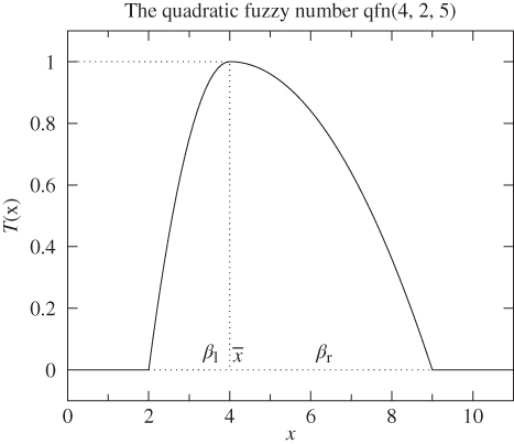
Figure 3.4 A quadratic fuzzy number.
3.1.5 Exponential Fuzzy Numbers
Exponential fuzzy numbers are yet another type of fuzzy numbers. Their membership function has the general form1:

Here ![]() and
and ![]() are the left and right spread of
are the left and right spread of ![]() , respectively, and
, respectively, and ![]() represents a tolerance value. We will specify an exponential fuzzy number using the notation
represents a tolerance value. We will specify an exponential fuzzy number using the notation ![]() . Figure 3.5 depicts an exponential fuzzy number.
. Figure 3.5 depicts an exponential fuzzy number.
3.1.6  –
– Fuzzy Numbers
Didier Dubois and Henri Prade [109] have introduced a special form of fuzzy numbers that are dubbed ![]() –
–![]() fuzzy numbers. The name derives from the fact that the graph of the membership function consists of two parts: the left and the right curve that meet at point
fuzzy numbers. The name derives from the fact that the graph of the membership function consists of two parts: the left and the right curve that meet at point ![]() . Figure 3.6 shows a typical example of an
. Figure 3.6 shows a typical example of an ![]() –
–![]() fuzzy number. In general, the membership function of an
fuzzy number. In general, the membership function of an ![]() –
–![]() fuzzy number has the following form:
fuzzy number has the following form:

Figure 3.5 An exponential fuzzy number.
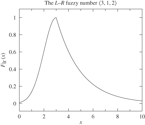
Figure 3.6 An  –
– fuzzy number.

Clearly, not all functions can be used in place of the ![]() and
and ![]() functions. In particular, these functions must have the following properties for all
functions. In particular, these functions must have the following properties for all ![]() :
:
 and
and  for all
  ;
; ;
; and
and  ; and
; and and
and  are decreasing in
  .
.
For example, in the case of the fuzzy number depicted in Figure 3.6, we have used:

3.1.7 Generalized Fuzzy Numbers
A generalized fuzzy number2 ![]() is a fuzzy subset of
is a fuzzy subset of ![]() that satisfies the following conditions:
that satisfies the following conditions:
 is a continuous mapping from
  to the closed interval
  ;
; when
when  ;
; is strictly increasing in
  ;
; when
when  ;
; is strictly decreasing in
  ;
; when
when  .
.
Here ![]() is supposed to be the degree of confidence of some expert's opinion. If
is supposed to be the degree of confidence of some expert's opinion. If ![]() , then the generalized fuzzy number
, then the generalized fuzzy number ![]() is called a normal trapezoidal fuzzy number. If
is called a normal trapezoidal fuzzy number. If ![]() and
and ![]() , then
, then ![]() is called a crisp interval. If
is called a crisp interval. If ![]() , then
, then ![]() is called a generalized triangular fuzzy number. If
is called a generalized triangular fuzzy number. If ![]() and
and ![]() , then
, then ![]() is called a real number.
is called a real number.
3.2 Arithmetic of Fuzzy Numbers
Given two fuzzy numbers ![]() and
and ![]() , does it make sense to compute their sum, their difference, their product, and their quotient? The answer to this question is that all four arithmetical operations have been extended so to make the operations
, does it make sense to compute their sum, their difference, their product, and their quotient? The answer to this question is that all four arithmetical operations have been extended so to make the operations ![]() ,
, ![]() ,
, ![]() , and
, and ![]() meaningful when
meaningful when ![]() and
and ![]() are fuzzy numbers. In particular, there are two methods to compute the operation
are fuzzy numbers. In particular, there are two methods to compute the operation ![]() : one method is defined using operations on intervals, while the other method is using the extension principle.
: one method is defined using operations on intervals, while the other method is using the extension principle.
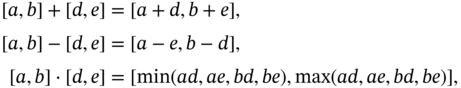
3.2.1 Interval Arithmetic
Before we can proceed to the presentation of the methods of doing fuzzy arithmetic, we first have to learn some of the basics of interval arithmetic. In general, if ![]() and
and ![]() are two closed intervals and
are two closed intervals and ![]() denotes any of the four arithmetic operations, then
denotes any of the four arithmetic operations, then
For example, if ![]() and
and ![]() and
and ![]() denotes addition, then
denotes addition, then
which equals ![]() , because the end points are elements of the intervals and from this it follows that
, because the end points are elements of the intervals and from this it follows that ![]() and
and ![]() .
.
Using Eq. (3.2), the four arithmetic operations on closed intervals are defined as follows:
and, provided that ![]() ,
,

Any real number ![]() can be considered as a degenerated interval
can be considered as a degenerated interval ![]() . Thus, if
. Thus, if ![]() ,
, ![]() , and
, and ![]() , then
, then ![]() because
because ![]() , and
, and ![]() because
because ![]() .
.
3.2.2 Interval Arithmetic and α‐Cuts
All α‐cuts of a fuzzy number are closed and bounded intervals. Assume that ![]() and
and ![]() are two fuzzy numbers and
are two fuzzy numbers and ![]() is one of the four arithmetic operations. Then, the fuzzy set
is one of the four arithmetic operations. Then, the fuzzy set ![]() is defined using its α‐cut
is defined using its α‐cut ![]() as
as
for all ![]() . In case we want to divide two fuzzy numbers, it is necessary to ensure that
. In case we want to divide two fuzzy numbers, it is necessary to ensure that ![]() for all
for all ![]() . In general, it would be useful to be able to use all α‐cuts. For instance, if
. In general, it would be useful to be able to use all α‐cuts. For instance, if ![]() and
and ![]() , then
, then
Of course, here we have shown how to compute specific α‐cuts and not how to compute new fuzzy numbers. However, we know from Theorem 2.3.2 that the union of all α‐cuts of some fuzzy set makes up the set itself. Thus, knowing all α‐cuts of the sum of two fuzzy numbers means that we can easily compute the new fuzzy number.
3.2.3 Fuzzy Arithmetic and the Extension Principle
The four arithmetic operations between fuzzy numbers can also be defined using the extension principle. The idea is that operations on real numbers are extended into operations on fuzzy real numbers. Assume that ![]() and
and ![]() are two fuzzy numbers. Then, we can define the four arithmetic operations between
are two fuzzy numbers. Then, we can define the four arithmetic operations between ![]() and
and ![]() for all
for all ![]() as follows:
as follows:

The technique described for discrete fuzzy numbers can be extended to nondiscrete fuzzy numbers, but it is more difficult to proceed.
3.2.4 Fuzzy Arithmetic of Triangular Fuzzy Numbers
For certain kinds of fuzzy numbers, there are special methods that can be used to compute any of the four arithmetic operations easily. This is true for triangular fuzzy numbers. Given two triangular fuzzy numbers ![]() and
and ![]() , then the four arithmetic operations are defined as follows [70]:
, then the four arithmetic operations are defined as follows [70]:
- Addition.
 ;
; - Subtraction.
 ;
; - Multiplication.
 ;
; - Division.
 .
.
3.2.5 Fuzzy Arithmetic of Generalized Fuzzy Numbers
Assume that ![]() and
and ![]() are two generalized fuzzy numbers. Then, their addition is defined as follows:
are two generalized fuzzy numbers. Then, their addition is defined as follows:

Also, ![]() is defined as follows:
is defined as follows:
The multiplication ![]() is equal to
is equal to ![]() , where
, where

The inverse of the fuzzy number ![]() is
is

where ![]() ,
, ![]() ,
, ![]() , and
, and ![]() are all nonzero positive numbers or nonzero negative numbers. If
are all nonzero positive numbers or nonzero negative numbers. If ![]() ,
, ![]() ,
, ![]() ,
, ![]() ,
, ![]() ,
, ![]() ,
, ![]() , and
, and ![]() are all nonzero positive real numbers, then
are all nonzero positive real numbers, then

It was demonstrated [85] that these operations are problematic (e.g. addition does not yield the exact value). Thus, a more general description of generalized fuzzy numbers was proposed. In particular, the number ![]() is written as follows:
is written as follows:

where ![]() is the degree of confidence with respect to a decision‐maker's opinion. The various arithmetic operations are defined as follows:
is the degree of confidence with respect to a decision‐maker's opinion. The various arithmetic operations are defined as follows:
- Addition.
 , where

- Subtraction.
 , where

- Multiplication.
 , where
- Division.
 , where

and
 ,
,  ,
,  ,
,  ,
,  ,
,  ,
,  , and
, and  are positive real numbers.
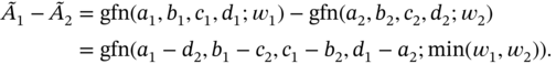
3.2.6 Comparing Fuzzy Numbers
Unfortunately, we cannot directly compare two fuzzy numbers ![]() and
and ![]() . However, we can compare them indirectly by using the operations
. However, we can compare them indirectly by using the operations ![]() and
and ![]() , that are obtained from the known
, that are obtained from the known ![]() and
and ![]() operations by using the extension principle as follows:
operations by using the extension principle as follows:

for ![]() . One can use these definitions to compute the minimum and maximum of any two fuzzy numbers, but nevertheless the computations can be easy only in certain cases. Thus, we need a better mechanism to compute these two operations. Chih‐Hui Chiu and Wen‐June Wang [74] proved two theorems that make the computation of these two operations easier. The first theorem can be used to compute
. One can use these definitions to compute the minimum and maximum of any two fuzzy numbers, but nevertheless the computations can be easy only in certain cases. Thus, we need a better mechanism to compute these two operations. Chih‐Hui Chiu and Wen‐June Wang [74] proved two theorems that make the computation of these two operations easier. The first theorem can be used to compute ![]() .
.
The second theorem can be used to compute ![]() .
.
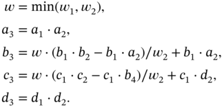
Dug Hun Hong and Kyung Tae Kim [163] found another easier way to compute the minimum and maximum of many fuzzy numbers at the same time. Their result is based on a theorem that uses the following notation:

3.3 Linguistic Variables
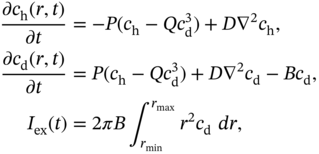
The concept of a linguistic variable4 was introduced by Zadeh [311–313]. According to Zadeh, a linguistic variable is a special kind of variable whose values are not numbers but words or, more generally, sentences in a natural language (e.g. English or Greek). For instance, the temperature of a room is a linguistic variable whose linguistic values include the terms “freezing,” “very cold,” “cold,” “cool,” “mild,” “moderate,” “warm,” “very warm,” and “hot.” Other examples of linguistic variables are the age of people, where possible linguistic values include the terms “young,” “old,” and “middle‐aged,” and the speed of a car, where possible linguistic values include the terms “fast,” “slow,” and “stationary.”
More formally, a linguistic variable is characterized by a quintuple ![]() , where
, where ![]() is the name of the variable,
is the name of the variable, ![]() is the set of terms of
is the set of terms of ![]() , that is, a set of linguistic values of
, that is, a set of linguistic values of ![]() , which are fuzzy sets on the universe
, which are fuzzy sets on the universe ![]() ,
, ![]() is a syntactic rule for generating the names of values of
is a syntactic rule for generating the names of values of ![]() , and
, and ![]() is a semantic rule for associating each value with its meaning, that is, the membership function that characterizes the fuzzy set. Figure 3.8 depicts the linguistic variable temperature.
is a semantic rule for associating each value with its meaning, that is, the membership function that characterizes the fuzzy set. Figure 3.8 depicts the linguistic variable temperature.
Any word like the word “very” that modifies a linguistic value like “cold” is called a linguistic hedge. For example, the words “quite,” “very very,” “not so,” etc., all count as linguistic hedges. A linguistic hedge can either intensify or lessen the meaning of a linguistic value. For example, if ![]() is the fuzzy set associated with the linguistic value “cold,” then
is the fuzzy set associated with the linguistic value “cold,” then ![]() could be the fuzzy set associated with the linguistic value “very cold.” Similarly, if
could be the fuzzy set associated with the linguistic value “very cold.” Similarly, if ![]() is the fuzzy set associated with the linguistic value “hot,” then
is the fuzzy set associated with the linguistic value “hot,” then ![]() could be the fuzzy set associated with the linguistic value “very hot.” The linguistic hedges and the atomic linguistic variable set (i.e. the “basic” words that characterize a linguistic variable) are put together to create the linguistic values. And this is exactly a possible syntactic rule for generating linguistic values.
could be the fuzzy set associated with the linguistic value “very hot.” The linguistic hedges and the atomic linguistic variable set (i.e. the “basic” words that characterize a linguistic variable) are put together to create the linguistic values. And this is exactly a possible syntactic rule for generating linguistic values.
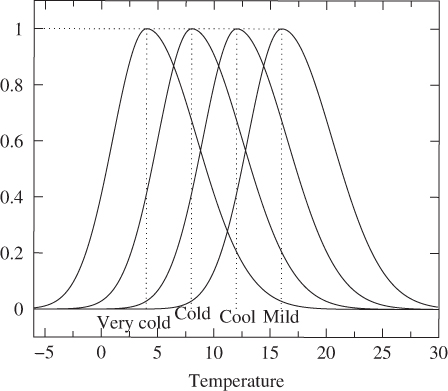
Figure 3.8 Room temperature as a linguistic variable quantified by some linguistic values.
3.4 Fuzzy Equations5
A fuzzy equation is one where both the unknown variables and the coefficients are fuzzy numbers. For example, the equation
where ![]() ,
, ![]() , and
, and ![]() are triangular fuzzy numbers, is the simplest possible fuzzy equation. It is rather tempting to try to solve this equation using techniques we use to solve ordinary algebraic equations. However, this is not possible because
are triangular fuzzy numbers, is the simplest possible fuzzy equation. It is rather tempting to try to solve this equation using techniques we use to solve ordinary algebraic equations. However, this is not possible because ![]() and so
and so ![]() ! For example, if
! For example, if ![]() , then
, then ![]() , as can be easily verified using the method described in Section 3.2.4.
, as can be easily verified using the method described in Section 3.2.4.
3.4.1 Solving the Fuzzy Equation 
In what follows, we present three methods to solve Eq. (3.5).
3.4.1.1 The Classical Method
This method can be used to compute the solution to an equation, when a solution exists. Assume that ![]() ,
, ![]() ,
, ![]() , and
, and ![]() ,
, ![]() . Then, we replace the variables in Eq. (3.5) with the α‐cuts:
. Then, we replace the variables in Eq. (3.5) with the α‐cuts:
Next, we need to solve this equation for ![]() and
and ![]() using interval arithmetic (see Section 3.2.1). When the intervals
using interval arithmetic (see Section 3.2.1). When the intervals ![]() define the α‐cuts of a fuzzy number, then we get the solution to Eq. (3.5). Note that
define the α‐cuts of a fuzzy number, then we get the solution to Eq. (3.5). Note that ![]() and
and ![]() specify α‐cuts of a fuzzy number when
specify α‐cuts of a fuzzy number when
 and
and  are continuous;
 is monotonically increasing for
  ;
; is monotonically decreasing for
  ; and
; and .
.
There is no guarantee that this procedure will yield a solution to Eq. (3.5), but if it does produce a solution, then this will satisfy the initial equation.
Although we managed to solve this equation using this method, most equations cannot be solved using this technique. Fortunately, there are two more methods which can produce approximate solutions to Eq. (3.5).
3.4.1.2 The Extension Principle Method
As the name of this method suggests, this method uses the extension principle to solve equation ![]() . The method is based on a procedure that is used to extend any crisp function
. The method is based on a procedure that is used to extend any crisp function ![]() to a fuzzy function
to a fuzzy function ![]() . According to this procedure, the crisp function
. According to this procedure, the crisp function ![]() is extended to its fuzzy counterpart
is extended to its fuzzy counterpart ![]() as follows:
as follows:

This equation defines the membership function of ![]() for any triangular fuzzy number
for any triangular fuzzy number ![]() in
in ![]() . Also, if
. Also, if ![]() is continuous, then there is a way to compute the α‐cuts of
is continuous, then there is a way to compute the α‐cuts of ![]() . Assume that
. Assume that ![]() . Then,
. Then,
If we have a crisp function with two independent variables, then we assume that ![]() , where
, where ![]() and
and ![]() . Then, we extend
. Then, we extend ![]() to
to ![]() as follows:
as follows:
Provided ![]() is continuous, we can compute the α‐cuts with the following equations:
is continuous, we can compute the α‐cuts with the following equations:
As an exercise, explain how one can fuzzify a crisp function with four independent variables.
The second method by which we try to solve Eq. (3.5), assumes that the crisp solution is a function of three independent variables. Therefore, all that we have to do is to fuzzify the “function” ![]() using the function fuzzification procedure we just described. Clearly, the solution we are looking for is the fuzzy number
using the function fuzzification procedure we just described. Clearly, the solution we are looking for is the fuzzy number ![]() , where zero does not belong to the support of
, where zero does not belong to the support of ![]() . The fuzzy number
. The fuzzy number ![]() can be computed using the following equation:
can be computed using the following equation:
Since ![]() is continuous, we can compute the α‐cuts
is continuous, we can compute the α‐cuts ![]() , where
, where
Clearly, the α‐cuts will be ![]() . The solution will be a triangular fuzzy number. However, there is no guarantee that the computed solution will satisfy the initial equation. If
. The solution will be a triangular fuzzy number. However, there is no guarantee that the computed solution will satisfy the initial equation. If ![]() does not exist, then the solution of the equation is
does not exist, then the solution of the equation is ![]() !
!
3.4.1.3 The α‐Cuts Method
A third method to solve equation ![]() is to use α‐cuts and interval arithmetic. In particular, the solution of the equation is assumed to be
is to use α‐cuts and interval arithmetic. In particular, the solution of the equation is assumed to be
This equation can be simplified into

or

if ![]() for all
for all ![]() . This method always yields the solution
. This method always yields the solution
but, again, there is no guarantee that the computed solution will satisfy the initial equation. If ![]() does not exist and it is difficult to get
does not exist and it is difficult to get ![]() , then we can use
, then we can use ![]() as an approximate solution.
as an approximate solution.
3.4.2 Solving the Fuzzy Equation 
The fuzzy quadratic equation has the following form:
For triangular fuzzy numbers ![]() ,
, ![]() ,
, ![]() , and
, and ![]() , the solution of this equation will be also a triangular fuzzy number. The fuzzy quadratic equation does not have the form
, the solution of this equation will be also a triangular fuzzy number. The fuzzy quadratic equation does not have the form ![]() just because the left‐hand side of this equation can never be exactly equal to zero. If we allow complex solutions, then the crisp equation
just because the left‐hand side of this equation can never be exactly equal to zero. If we allow complex solutions, then the crisp equation ![]() has two solutions, which implies that the fuzzy equation might have solutions that are fuzzy complex numbers, nonetheless we are not interested in fuzzy complex solutions. As in the case of the equation
has two solutions, which implies that the fuzzy equation might have solutions that are fuzzy complex numbers, nonetheless we are not interested in fuzzy complex solutions. As in the case of the equation ![]() , there are three methods to solve Eq. (3.15).
, there are three methods to solve Eq. (3.15).
3.4.2.1 The Classical Method
Assume that ![]() ,
, ![]() ,
, ![]() ,
, ![]() , and
, and ![]() . Then, we substitute these α‐cuts into Eq. (3.15) and solve for
. Then, we substitute these α‐cuts into Eq. (3.15) and solve for ![]() and
and ![]() . In order to proceed, we need to know whether
. In order to proceed, we need to know whether ![]() ,
, ![]() , and
, and ![]() . Suppose that all these numbers are positive. Then,
. Suppose that all these numbers are positive. Then,

The solution ![]() exists if the α‐cuts
exists if the α‐cuts ![]() , where
, where

are of a triangular fuzzy number. This means that ![]() and
and ![]() , for
, for ![]() and
and ![]() . In addition, the solutions must be real numbers, so this means that
. In addition, the solutions must be real numbers, so this means that
Naturally, if ![]() and
and ![]() or
or ![]() and
and ![]() , we may get different results, provided all conditions are met.
, we may get different results, provided all conditions are met.
3.4.2.2 The Extension Principle Method
This solution fuzzifies the quantities ![]() and
and ![]() and the α‐cut of
and the α‐cut of ![]() , when we are working with
, when we are working with ![]() , is
, is ![]() , where
, where
for ![]() .
.
3.4.2.3 The α‐Cuts Method
This method is employed when it is difficult to compute the ![]() and
and ![]() in the previous equations. The solution
in the previous equations. The solution ![]() is computed by substitution of
is computed by substitution of ![]() ,
, ![]() ,
, ![]() , and
, and ![]() into
into ![]() or
or ![]() . Here, we work with
. Here, we work with ![]() , and we assume that the α‐cut of
, and we assume that the α‐cut of ![]() is
is ![]() , where
, where

![]() .
.
3.5 Fuzzy Inequalities
A fuzzy inequality is an expression like ![]() or like
or like ![]() , where
, where ![]() ,
, ![]() , and
, and ![]() are triangular fuzzy numbers. However, the problem here is, what do the expressions
are triangular fuzzy numbers. However, the problem here is, what do the expressions ![]() and
and ![]() really mean? Unfortunately, there is no unique definition and this means that a possible solution will depend on how we choose to define these two relational operators.
really mean? Unfortunately, there is no unique definition and this means that a possible solution will depend on how we choose to define these two relational operators.
A number of different definitions is presented in [44], but it seems there is no standard definition. Here is a simple definition:
Based on this, we agree that ![]() if
if ![]() , but
, but ![]() , where
, where ![]() is a fixed number, such that
is a fixed number, such that ![]() . Let us say that
. Let us say that ![]() . Then,
. Then, ![]() if
if ![]() and
and ![]() . We write
. We write ![]() when both
when both ![]() and
and ![]() are not true. Moreover,
are not true. Moreover, ![]() means that
means that ![]() or that
or that ![]() .
.
In order to solve the inequality ![]() , we first try to compute the number
, we first try to compute the number ![]() . Suppose we are going to use α‐cuts and interval arithmetic to compute
. Suppose we are going to use α‐cuts and interval arithmetic to compute ![]() . Then, the solution for
. Then, the solution for ![]() to
to ![]() or
or ![]() depends on the definition of “
depends on the definition of “![]() .” However, since there is no standard definition but only proposals, there is no reason to further discuss possible solutions.
.” However, since there is no standard definition but only proposals, there is no reason to further discuss possible solutions.
3.6 Constructing Fuzzy Numbers
We have shown how to deal with fuzzy numbers, but we have said nothing about how one can actually construct them from real‐world data. Chi‐Bin Cheng [73] presented a relatively simple method that can be used to construct a triangular fuzzy number. In particular, he explained how one can construct a triangular fuzzy number ![]() from the grades given to
from the grades given to ![]() , which can be an object, a performance, etc., by a group of experts. We can assume that each expert graded
, which can be an object, a performance, etc., by a group of experts. We can assume that each expert graded ![]() with a number in the range from 0 to
with a number in the range from 0 to ![]() . Moreover,
. Moreover, ![]() are the scores that
are the scores that ![]() different experts gave to
different experts gave to ![]() . In addition, we require that
. In addition, we require that ![]() for at least one pair of grades
for at least one pair of grades ![]() and
and ![]() .
.
The first thing we would like to compute is the number ![]() . For this, we build the
. For this, we build the ![]() matrix
matrix ![]() , where each
, where each ![]() . This matrix holds the distances between various
. This matrix holds the distances between various ![]() , and it is used to locate
, and it is used to locate ![]() . The average of the relative distances, for each
. The average of the relative distances, for each ![]() , is given by
, is given by ![]() . This average distance is used to measure the proximity of
. This average distance is used to measure the proximity of ![]() to
to ![]() . Next, we want to determine the degree of importance of each
. Next, we want to determine the degree of importance of each ![]() . So, we build an
. So, we build an ![]() pair‐wise comparison matrix
pair‐wise comparison matrix ![]() , where
, where

Because ![]() is obtained from a comparison of distances, it turns out that it is perfectly consistent. Assume that
is obtained from a comparison of distances, it turns out that it is perfectly consistent. Assume that ![]() is the true degree of importance of
is the true degree of importance of ![]() . Then, because of the consistency of
. Then, because of the consistency of ![]() ,
,

Suppose that ![]() is a column vector of
is a column vector of ![]() , where
, where ![]() . Then,
. Then,
which means that ![]() is an eigenvalue of
is an eigenvalue of ![]() and
and ![]() is the corresponding eigenvector. It holds that
is the corresponding eigenvector. It holds that

and we conclude that

From this we can finally compute ![]() :
:

Now we need to compute ![]() and
and ![]() .
.
This last equation can be written as follows:
Also, let ![]() be
be
These last two equations can be solved to yield

Obviously, ![]() and
and ![]() .
.
We use the average deviation that is calculated from the sample scores to approximate the value of ![]() :
:

The quantity ![]() can be computed approximately as follows. Assume that
can be computed approximately as follows. Assume that ![]() is the weighted average of the scores that are less than
is the weighted average of the scores that are less than ![]() and
and ![]() the weighted average of the scores that are greater than
the weighted average of the scores that are greater than ![]() . Also, let
. Also, let
Next, we compute ![]() and
and ![]() :
:

Finally, we can approximately compute ![]() by
by

Assume that ![]() ,
, ![]() , for all
, for all ![]() and
and ![]() . Then, the method described cannot be used since this condition violates the assumptions of the method. However, the membership function of the corresponding fuzzy number can be constructed easily:
. Then, the method described cannot be used since this condition violates the assumptions of the method. However, the membership function of the corresponding fuzzy number can be constructed easily:

The scores given by the experts are between 0 and ![]() , therefore, the support of a fuzzy number constructed from these scores cannot be outside this range. Thus, the triangular fuzzy number is defined as follows:
, therefore, the support of a fuzzy number constructed from these scores cannot be outside this range. Thus, the triangular fuzzy number is defined as follows:

3.7 Applications of Fuzzy Numbers
There are many nontrivial applications of fuzzy numbers and Michael Hanss's monograph [159] describes some very interesting applications. In this section, we present a few applications of fuzzy numbers so as to demonstrate their usefulness.
3.7.1 Simulation of the Human Glucose Metabolism
It is an undeniable fact that diabetes mellitus type I can seriously affect the quality of a patient's life. Since diabetes is the result of a problematic human glucose metabolism, it is of paramount importance to know the main characteristics of glucose metabolism. Naturally, we first need to develop a mathematical model of the metabolism and then use it in simulations so to check its usefulness. Michael Hanss and Oliver Nehls [160] examine such a model and find ways to improve the model by introducing fuzzy numbers. First, let us briefly present the model and then we can see how fuzzy numbers can be introduced.
Generally speaking, the human glucose metabolism model for patients with diabetes mellitus type I is divided into two parts: (i) the part that describes the inflow ![]() of insulin into blood as a result of a subcutaneous insulin injection, and (ii) the part that describes the inflow
of insulin into blood as a result of a subcutaneous insulin injection, and (ii) the part that describes the inflow ![]() of glucose into blood as a result of food consumption. The second part is divided into two submodels: (i) the submodel that describes metabolisms in the stomach, and (ii) the submodel that describes the metabolism in the intestine. The outputs of these models are combined in a simplified model to predict the amount of in‐blood glucose
of glucose into blood as a result of food consumption. The second part is divided into two submodels: (i) the submodel that describes metabolisms in the stomach, and (ii) the submodel that describes the metabolism in the intestine. The outputs of these models are combined in a simplified model to predict the amount of in‐blood glucose ![]() at time
at time ![]() .
.
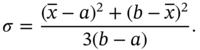
When a patient injects insulin, it appears in two modifications in the subcutaneous depot. These are described by a hemisphere with radial coordinate ![]() : as dimer insulin with concentration
: as dimer insulin with concentration ![]() and as hexamer insulin with concentration
and as hexamer insulin with concentration ![]() . The uptake of insulin into the blood is only affected by dimer insulin. However, the injected external insulin is a solution of pure hexamer insulin. The following equations describe the model:
. The uptake of insulin into the blood is only affected by dimer insulin. However, the injected external insulin is a solution of pure hexamer insulin. The following equations describe the model:
where
and the model parameters

and the initial and boundary conditions
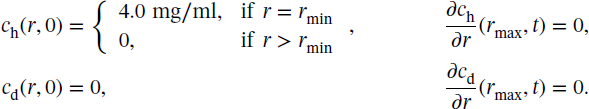
The model for the concentration ![]() of carbohydrates in the stomach of volume
of carbohydrates in the stomach of volume ![]() is given by
is given by

with the initial conditions
and the parameters


The input parameters ![]() ,
, ![]() , and
, and ![]() designate the amount of carbohydrates, proteins, and fat in the ingested meal.
designate the amount of carbohydrates, proteins, and fat in the ingested meal.
The model for the concentration ![]() of carbohydrates in the intestine of radius
of carbohydrates in the intestine of radius ![]() and length
and length ![]() is given by
is given by

with the initial and boundary conditions

and the parameters

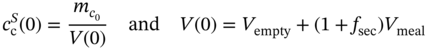
The simplified model for the amount of in‐blood glucose ![]() is described below:
is described below:

The sensitivity parameters ![]() ,
, ![]() , and
, and ![]() can be considered as constants for a multiple
can be considered as constants for a multiple ![]() of the time interval
of the time interval ![]() . Typically, the time interval is chosen to be
. Typically, the time interval is chosen to be ![]() and the sensitivity parameters are considered as constant for about one hour, that is,
and the sensitivity parameters are considered as constant for about one hour, that is, ![]() .
.
From the description so far, it is obvious that the parameters ![]() and
and ![]() have values that lie within a specific range, which means that they are vague values by definition. In addition, it is next to impossible to predetermine the amount of carbohydrates
have values that lie within a specific range, which means that they are vague values by definition. In addition, it is next to impossible to predetermine the amount of carbohydrates ![]() . So the model needs at least three fuzzy numbers that are represented by quasi‐Gaussian fuzzy numbers:
. So the model needs at least three fuzzy numbers that are represented by quasi‐Gaussian fuzzy numbers:

The various values have been chosen based on the data presented in the original model, while ![]() and the nutritional content of carbohydrates in the ingested food is usually an integer multiple of the bread unit. Finally, the initial condition for the in‐blood glucose is set to
and the nutritional content of carbohydrates in the ingested food is usually an integer multiple of the bread unit. Finally, the initial condition for the in‐blood glucose is set to
3.7.2 Estimation of an Ongoing Project's Completion Time
For any project it is a good planning strategy to try to anticipate all possible cases that may delay its realization. However, no matter how good we plan a project, it is quite possible that some unexpected things may occur that might eventually delay the realization of the project. Therefore, we need a tool that can be used to analyze a situation and make some sort of predictions. The “obvious” solution is to use probability theory, as noted by Dorota Kuchta [184]. However, it seems that this approach is not useful since it assumes that we can verify certain hypotheses about the probability distributions of activity duration times. Clearly, if we know these times in advance, then we do not need probability theory. As an alternative approach to the solution of this problem, Kuchta suggested the use of fuzzy numbers since they make it easy to describe several criteria that influence the actual duration of a project's activities.
Kuchta's fuzzy numbers are a special form of triangular fuzzy numbers. In particular, she defines a fuzzy number ![]() as a triplet
as a triplet ![]() whose analytic form is as follows:
whose analytic form is as follows:

Here ![]() is called the mean value, while the variability measures
is called the mean value, while the variability measures ![]() and
and ![]() measure the uncertainty linked to the assumption that the unknown magnitude
measure the uncertainty linked to the assumption that the unknown magnitude ![]() will be equal to
will be equal to ![]() .
.
3.7.2.1 Model of a Project
Each project should be understood as a set of activities
Clearly, the members of this set may have dependencies between them (e.g. ![]() should happen before
should happen before ![]() , or
, or ![]() and
and ![]() use the same resources, etc.). At the beginning, we provide an estimation of each activity's duration, but when the project is implemented, the mean value of an activity's duration may depend on a number of factors. Such factors are the weather, the mood in the activity team, the skills of the activity team, the attitude of certain stakeholders, etc. Unfortunately, most of these factors cannot be measured, although they may strongly influence the duration of an activity. The set of all these factors will be
use the same resources, etc.). At the beginning, we provide an estimation of each activity's duration, but when the project is implemented, the mean value of an activity's duration may depend on a number of factors. Such factors are the weather, the mood in the activity team, the skills of the activity team, the attitude of certain stakeholders, etc. Unfortunately, most of these factors cannot be measured, although they may strongly influence the duration of an activity. The set of all these factors will be
For each ![]() , we will denote by
, we will denote by ![]() the impact of
the impact of ![]() on the estimation of the mean values of the durations of project activities at time
on the estimation of the mean values of the durations of project activities at time ![]() , where
, where ![]() is a point beyond which the project cannot go (Kuchta calls it time horizon) and 0 is the planning phase of the project. Apart from these factors, it is quite possible to have factors that affect the uncertainty (variability) in the estimation of an activity's duration. The set of these “other” factors will be written as follows:
is a point beyond which the project cannot go (Kuchta calls it time horizon) and 0 is the planning phase of the project. Apart from these factors, it is quite possible to have factors that affect the uncertainty (variability) in the estimation of an activity's duration. The set of these “other” factors will be written as follows:
It is quite possible that ![]() is in an one‐to‐one correspondence with
is in an one‐to‐one correspondence with ![]() . However, this does not imply that in all cases, the sets are in an one‐to‐one correspondence. Also, all
. However, this does not imply that in all cases, the sets are in an one‐to‐one correspondence. Also, all ![]() will represent the impact of the corresponding factors on the uncertainty of the estimates of the duration of the activities of the project at a given moment
will represent the impact of the corresponding factors on the uncertainty of the estimates of the duration of the activities of the project at a given moment ![]() . These two sets are clearly different, and the elements of the first one affect the duration of an activity and can be used to determine the most possible value of the duration. The elements of the second set affect the variability of the estimate around the mean value. For instance, in construction projects, the weather plays a decisive role in the determination of the duration of certain activities and may affect the mean value of the estimated completion time entirely (forecasts of long rainy periods or long sunny periods often affect the mean values in different ways). However, other factors like technical problems or the experience of the team members, do not have such a strong impact on the completion of a project but affect the precise determination of the completion time. Therefore, one should take into account their variability in both directions.
. These two sets are clearly different, and the elements of the first one affect the duration of an activity and can be used to determine the most possible value of the duration. The elements of the second set affect the variability of the estimate around the mean value. For instance, in construction projects, the weather plays a decisive role in the determination of the duration of certain activities and may affect the mean value of the estimated completion time entirely (forecasts of long rainy periods or long sunny periods often affect the mean values in different ways). However, other factors like technical problems or the experience of the team members, do not have such a strong impact on the completion of a project but affect the precise determination of the completion time. Therefore, one should take into account their variability in both directions.
For each activity ![]() ,
, ![]() will be the estimate of the duration of this activity at a moment
will be the estimate of the duration of this activity at a moment ![]() before this activity has been finished:
before this activity has been finished:
where ![]() ,
, ![]() , and
, and ![]() are invertible functions from and into the set of nonnegative real numbers,
are invertible functions from and into the set of nonnegative real numbers, ![]() , and
, and ![]() and
and ![]() are not necessarily different indices from the set
are not necessarily different indices from the set ![]() . From this equation, it is clear that all three parameters, that is, the mean value of the estimates as well as its variability measures, depend on exactly one parameter. Although this may seem like a limitation, in most real‐life cases, one major factor can be selected: one for the mean value and one for each of the two variability measures. Also, according to Eq. (3.16) the duration of each activity is vague.
. From this equation, it is clear that all three parameters, that is, the mean value of the estimates as well as its variability measures, depend on exactly one parameter. Although this may seem like a limitation, in most real‐life cases, one major factor can be selected: one for the mean value and one for each of the two variability measures. Also, according to Eq. (3.16) the duration of each activity is vague.
When realizing a project, one should be able to update the estimates of the duration of activities which have not been started yet, and thus to update the estimate of the total duration time of the project. For this we need a set of selected control moments
where ![]() and
and ![]() . Depending on the nature of the project, the intervals
. Depending on the nature of the project, the intervals ![]() for
for ![]() might be smaller if the project is risky, or they might be bigger if the project is not risky. At a moment
might be smaller if the project is risky, or they might be bigger if the project is not risky. At a moment ![]() ,
, ![]() ,
, ![]() will denote the estimated total completion time of the project at this given moment.
will denote the estimated total completion time of the project at this given moment. ![]() is actually the maximum of the estimated lengths of all the paths in the project network, using the actual completion time of the activities which have been completed at moment
is actually the maximum of the estimated lengths of all the paths in the project network, using the actual completion time of the activities which have been completed at moment ![]() , and using the estimated duration time of the activities that have not been completed in the form of fuzzy numbers derived from Eq. (3.16):
, and using the estimated duration time of the activities that have not been completed in the form of fuzzy numbers derived from Eq. (3.16):
In order to get a reliable and informative estimate ![]() at each control moment
at each control moment ![]() , it is necessary to have the best possible estimates
, it is necessary to have the best possible estimates ![]() of the durations of those activities
of the durations of those activities ![]() that have not been completed at
that have not been completed at ![]() . Kuchta has proposed an algorithm for updating the estimates
. Kuchta has proposed an algorithm for updating the estimates ![]() , but we will not describe it here. Our purpose was to show the use of fuzzy numbers in specific problems and not to show how specific problems can be solved completely.
, but we will not describe it here. Our purpose was to show the use of fuzzy numbers in specific problems and not to show how specific problems can be solved completely.
Exercises
- 3.1 Using Eq. (3.1) draw the triangular fuzzy numbers
 and
and  .
. - 3.2 Evaluate the following in interval arithmetic:
 ;
; ;
; ;
; ;
; .
.
- 3.3 Evaluate in interval arithmetic each of the following expressions:
 and
and  for
for  equal to each of the intervals
  ,
,  , and
, and  .
. - 3.4 Assume that
 and
and  . Find the fuzzy numbers
  ,
,  , and
, and  using the method described in Section 3.2.2.
 - 3.5 Redo the previous exercise using the method described in Section 3.2.4.
- 3.6 Complete Example 3.2.3 by calculating
 .
. - 3.7 Solve equation
 using the classical method when
  ,
,  , and
, and  .
. - 3.8 Verify that the equation
 has no classical solution when
  ,
,  , and
, and  .
. - 3.9 Assume that five experts assign the following five scores:

Construct the corresponding triangular fuzzy number.
Notes
- 1 We have used the definition presented in [159] to draw an exponential fuzzy number, but the result was totally wrong. However, the definition presented in [24] yielded a real exponential fuzzy number. Thus, the definition of exponential fuzzy numbers is borrowed from [24].
- 2 We use the description presented in [71], since the original paper that introduced generalized fuzzy numbers was not available to us.
- 3 For reasons of brevity, we just omit to specify the infinite numbers that have membership degree equal to zero.
- 4 This term has also been used in linguistics, where a linguistic variable is a linguistic item that has identifiable variants. For example, the fishing is sometimes pronounced as “fishin.” The final sound of this word is the linguistic variable (see Ref. [295] for a full discussion).
- 5 The exposition that follows is based on [44, 48].