12. Numerics
The purpose of computing is insight, not numbers.
– R. W. Hamming
... but for the student,
numbers are often the best road to insight.
– A. Ralston
• Advice
12.1. Introduction
C++ was not designed primarily with numeric computation in mind. However, numeric computation typically occurs in the context of other work – such as database access, networking, instrument control, graphics, simulation, and financial analysis – so C++ becomes an attractive vehicle for computations that are part of a larger system. Furthermore, numeric methods have come a long way from being simple loops over vectors of floating-point numbers. Where more complex data structures are needed as part of a computation, C++’s strengths become relevant. The net effect is that C++ is widely used for scientific, engineering, financial, and other computation involving sophisticated numerics. Consequently, facilities and techniques supporting such computation have emerged. This chapter describes the parts of the standard library that support numerics.
12.2. Mathematical Functions
In <cmath>, we find the standard mathematical functions, such as sqrt(), log(), and sin() for arguments of type float, double, and long double:
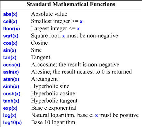
The versions for complex (§12.4) are found in <complex>. For each function, the return type is the same as the argument type.
Errors are reported by setting errno from <cerrno> to EDOM for a domain error and to ERANGE for a range error. For example:
void f()
{
errno = 0; // clear old error state
sqrt(-1);
if (errno==EDOM)
cerr << "sqrt() not defined for negative argument";
errno = 0; // clear old error state
pow(numeric_limits<double>::max(),2);
if (errno == ERANGE)
cerr << "result of pow() too large to represent as a double";
}
A few more mathematical functions are found in <cstdlib> and there is a separate ISO standard for special mathematical functions [C++Math,2010].
12.3. Numerical Algorithms
In <numeric>, we find a small set of generalized numerical algorithms, such as accumulate().
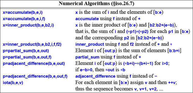
These algorithms generalize common operations such as computing a sum by letting them apply to all kinds of sequences and by making the operation applied to elements of those sequences a parameter. For each algorithm, the general version is supplemented by a version applying the most common operator for that algorithm. For example:
void f()
{
list<double> lst {1, 2, 3, 4, 5, 9999.99999};
auto s = accumulate(lst.begin(),lst.end(),0.0); // calculate the sum
cout << s << '
'; // print 10014.9999
}
These algorithms work for every standard-library sequence and can have operations supplied as arguments (§12.3).
12.4. Complex Numbers
The standard library supports a family of complex number types along the lines of the complex class described in §4.2.1. To support complex numbers where the scalars are single-precision floating-point numbers (floats), double-precision floating-point numbers (doubles), etc., the standard library complex is a template:
template<typename Scalar>
class complex {
public:
complex(const Scalar& re ={}, const Scalar& im ={});
// ...
};
The usual arithmetic operations and the most common mathematical functions are supported for complex numbers. For example:
void f(complex<float> fl, complex<double> db)
{
complex<long double> ld {fl+sqrt(db)};
db += fl*3;
fl = pow(1/fl,2);
// ...
}
The sqrt() and pow() (exponentiation) functions are among the usual mathematical functions defined in <complex> (§12.2).
12.5. Random Numbers
Random numbers are useful in many contexts, such as testing, games, simulation, and security. The diversity of application areas is reflected in the wide selection of random number generators provided by the standard library in <random>. A random number generator consists of two parts:
[1] an engine that produces a sequence of random or pseudo-random values.
[2] a distribution that maps those values into a mathematical distribution in a range.
Examples of distributions are uniform_int_distribution (where all integers produced are equally likely), normal_distribution (“the bell curve”), and exponential_distribution (exponential growth); each for some specified range. For example:
using my_engine = default_random_engine; // type of engine
using my_distribution = uniform_int_distribution<>; // type of distribution
my_engine re {}; // the default engine
my_distribution one_to_six {1,6}; // distribution that maps to the ints 1..6
auto die = bind(one_to_six,re); // make a generator
int x = die(); // roll the die: x becomes a value in [1:6]
The standard-library function bind() makes a function object that will invoke its first argument (here, one_to_six) given its second argument (here, re) as its argument (§11.5.1). Thus a call die() is equivalent to a call one_to_six(re).
Thanks to its uncompromising attention to generality and performance one expert has deemed the standard-library random number component “what every random number library wants to be when it grows up.” However, it can hardly be deemed “novice friendly.” The using statements makes what is being done a bit more obvious. Instead, I could just have written:
auto die = bind(uniform_int_distribution<>{1,6}, default_random_engine{});
Which version is the more readable depends entirely on the context and the reader.
For novices (of any background) the fully general interface to the random number library can be a serious obstacle. A simple uniform random number generator is often sufficient to get started. For example:
Rand_int rnd {1,10}; // make a random number generator for [1:10]
int x = rnd(); // x is a number in [1:10]
So, how could we get that? We have to get something like die() inside a class Rand_int:
class Rand_int {
public:
Rand_int(int low, int high) :dist{low,high} { }
int operator()() { return dist(re); } // draw an int
private:
default_random_engine re;
uniform_int_distribution<> dist;
};
That definition is still “expert level,” but the use of Rand_int() is manageable in the first week of a C++ course for novices. For example:
int main()
{
constexpr int max = 8;
Rand_int rnd {0,max}; // make a uniform random number generator
vector<int> histogram(max+1); // make a vector of appropriate size
for (int i=0; i!=200; ++i)
++histogram[rnd()]; // fill histogram with the frequencies of numbers [0:max]
for (int i = 0; i!=histogram.size(); ++i) { // write out a bar graph
cout << i << ' ';
for (int j=0; j!=histogram[i]; ++j) cout << '*';
cout << endl;
}
}
The output is a (reassuringly boring) uniform distribution (with reasonable statistical variation):
0 *********************
1 ****************
2 *******************
3 ********************
4 ****************
5 ***********************
6 **************************
7 ***********
8 **********************
9 *************************
There is no standard graphics library for C++, so I use “ASCII graphics.” Obviously, there are lots of open source and commercial graphics and GUI libraries for C++, but in this book I restrict myself to ISO standard facilities.
12.6. Vector Arithmetic
The vector described in §9.2 was designed to be a general mechanism for holding values, to be flexible, and to fit into the architecture of containers, iterators, and algorithms. However, it does not support mathematical vector operations. Adding such operations to vector would be easy, but its generality and flexibility precludes optimizations that are often considered essential for serious numerical work. Consequently, the standard library provides (in <valarray>) a vector-like template, called valarray, that is less general and more amenable to optimization for numerical computation:
template<typename T>
class valarray {
// ...
};
The usual arithmetic operations and the most common mathematical functions are supported for valarrays. For example:
void f(valarray<double>& a1, valarray<double>& a2)
{
valarray<double> a = a1*3.14+a2/a1; // numeric array operators *, +, /, and =
a2 += a1*3.14;
a = abs(a);
double d = a2[7];
// ...
}
For more details, see §12.6. In particular, valarray offers stride access to help implement multidimensional computations.
12.7. Numeric Limits
In <limits>, the standard library provides classes that describe the properties of built-in types – such as the maximum exponent of a float or the number of bytes in an int; see §12.7. For example, we can assert that a char is signed:
static_assert(numeric_limits<char>::is_signed,"unsigned characters!");
static_assert(100000<numeric_limits<int>::max(),"small ints!");
Note that the second assert (only) works because numeric_limits<int>::max() is a constexpr function (§1.7).
12.8. Advice
[1] The material in this chapter roughly corresponds to what is described in much greater detail in Chapter 40 of [Stroustrup,2013].
[2] Numerical problems are often subtle. If you are not 100% certain about the mathematical aspects of a numerical problem, either take expert advice, experiment, or do both; §12.1.
[3] Don’t try to do serious numeric computation using only the bare language; use libraries; §12.1.
[4] Consider accumulate(), inner_product(), partial_sum(), and adjacent_difference() before you write a loop to compute a value from a sequence; §12.3.
[5] Use std::complex for complex arithmetic; §12.4.
[6] Bind an engine to a distribution to get a random number generator; §12.5.
[7] Be careful that your random numbers are sufficiently random; §12.5.
[8] Use valarray for numeric computation when run-time efficiency is more important than flexibility with respect to operations and element types; §12.6.
[9] Properties of numeric types are accessible through numeric_limits; §12.7.
[10] Use numeric_limits to check that the numeric types are adequate for their use; §12.7.