
A recommendation system may be evaluated in two ways: offline and online. In the offline evaluation, also known as batch evaluation, the total history of user purchases is segregated into to random subsets, a large training subset (typically 80%) and a small testing subset (typically 20%). The matrix factorization procedure is then used on the 80% training subset to build a recommendation model.
Next, with this trained model, each record in the testing subset is evaluated against the model. If the model predicts that the user would purchase the item with sufficient confidence, and indeed the user purchased the item in the testing subset, then we record a "true positive." If the model predicts a purchase but the user did not purchase the item, we record a "false positive." If the model fails to predict a purchase, it is a "false negative," and if it predicts the user will not purchase the item and indeed they do not, we have a "true negative." With these true/false positive/negative counts, we can calculate precision and recall.
Precision is TP/(TP+FP), in other words, the ratio of purchases predicted by the model that were actual purchases. The recall is TP/(TP+FN), the ratio of actual purchases that the model predicted. Naturally, we want both measures to be high (near 1.0). Normally, precision and recall are a tradeoff: just by increasing the likelihood the system will predict a purchase (that is, lowering its required confidence level), we can earn a higher recall at the cost of precision. By being more discriminatory, we can lower recall while raising precision. Whether high precision or high recall is preferred depends on the application and business use case. For example, a higher precision but a lower recall would ensure that nearly all recommendations that are shown are actually purchased by the user. This could give the impression that the recommendation works really well, while it is possible the user would have purchased even more items if they were recommended.
On the other hand, a higher recall but lower precision could result in showing the user more recommendations, some or many of which they do not purchase. At different points in this sliding scale, the recommendation system is either showing the user too few or too many recommendations. Each application needs to find its ideal trade off, usually from trial and error and an online evaluation, described in the following text.
Another offline approach often used with explicit feedback, such as numeric ratings from product reviews, is root mean square error (RMSE), computed as:

In this case, N is the number of ratings in the testing subset, ![]() is the predicted rating, and
is the predicted rating, and ![]() is the actual rating. With this metric, lower is better. This metric is similar to the optimization criteria from the matrix factorization technique described previously. The goal there was to minimize the squared error by finding the optimal U and V matrices for approximating the original user-item matrix P.
is the actual rating. With this metric, lower is better. This metric is similar to the optimization criteria from the matrix factorization technique described previously. The goal there was to minimize the squared error by finding the optimal U and V matrices for approximating the original user-item matrix P.
Since we are interested in implicit ratings (1.0 or 0.0) rather than explicit numeric ratings, precision and recall are more appropriate measures than RMSE. Next, we will look at a way to calculate precision and recall in order to determine the best BM25 parameters for a dataset.
As a kind of offline evaluation, we next look at precision and recall for the MovieLens dataset (https://grouplens.org/datasets/movielens/20m/) across a range of BM25 parameters. This dataset has about 20 million ratings, scored 1-5, of thousands of movies by 138,000 users. We will turn these ratings into implicit data by considering any rating of 3.0 or higher to be positive implicit feedback and ratings below 3.0 to be non-existent feedback. If we do this, we will be left with about 10 million implicit values. The implicit library has this dataset built-in:
from implicit.datasets.movielens import get_movielens
_, ratings = get_movielens('20m')
We ignore the first returned value, the movie titles, of get_movielens() because we have no use for the titles.
Our goal is to study the impact of different BM25 parameters on precision and recall. We will iterate through several combinations of BM25 parameters and a confidence parameter. The confidence parameter will determine whether a predicted score is sufficiently high to predict that a particular user positively rated a particular movie. A low confidence parameter should produce more false positives, everything else being equal, than a high confidence parameter. We will save our output to a CSV file. We start by printing the column headers, then we iterate through each parameter combination. We also repeat each combination multiple times to get an average:
print("B,K1,Confidence,TP,FP,FN,Precision,Recall")
confidences = [0.0, 0.2, 0.4, 0.6, 0.8]
for iteration in range(5):
  seed = int(time.time())
  for conf in confidences:
    np.random.seed(seed)
    experiment(0.0, 0.0, conf)
  for conf in confidences:
    np.random.seed(seed)
    experiment("NA", "NA", conf)
  for B in [0.25, 0.50, 0.75, 1.0]:
    for K1 in [1.0, 3.0]:
      for conf in confidences:
        np.random.seed(seed)
        experiment(B, K1, conf)
Since B=0 is equivalent to K1=0 in BM25, we do not need to iterate over other values of B or K1 when either equals 0. Also, we will try cases with BM25 weighting turned off, indicated by B=K1=NA.
We will randomly hide (remove) some of the ratings and then attempt to predict them again. We do not want various parameter combinations to hide different random ratings. Rather, we want to ensure each parameter combination is tested on the same situation, so they are comparable. Only when we re-evaluate all the parameters in another iteration do we wish to choose a different random subset of ratings to hide. Hence, we establish a random seed at the beginning of each iteration and then use the same seed before running each experiment.
Our experiment function receives the parameters dictating the experiment. This function needs to load the data, randomly hide some of it, train a recommendation model, and then predict the implicit feedback of a subset of users for a subset of movies. Then, it needs to calculate precision and recall and print that information in CSV format.
While developing this function, we will make use of several NumPy features. Because we have relatively large datasets, we want to avoid, at all costs, any Python loops that manipulate the data. NumPy uses Basic Linear Algebra Subprograms (BLAS) to efficiently compute dot-products and matrix multiplications, possibly with parallelization (as with OpenBLAS). We should utilize NumPy array functions as much as possible to take advantage of these speedups.
We begin by loading the dataset and converting numeric ratings into implicit ratings:
def experiment(B, K1, conf, variant='20m', min_rating=3.0):
  # read in the input data file
  _, ratings = get_movielens(variant)
  ratings = ratings.tocsr()

  # remove things < min_rating, and convert to implicit dataset
  # by considering ratings as a binary preference only
  ratings.data[ratings.data < min_rating] = 0
  ratings.eliminate_zeros()
  ratings.data = np.ones(len(ratings.data))
The 3.0+ ratings are very sparse. Only 0.05% of values in the matrix are non-zero after converting to implicit ratings. Thus, we make extensive use of SciPy's sparse matrix support. There are various kinds of sparse matrix data structures: compressed sparse row matrix (CSR), and row-based linked-list sparse matrix (LIL), among others. The CSR format allows us to directly access the data in the matrix as a linear array of values. We set all values to 1.0 to construct our implicit scores.
Next, we need to hide some ratings. To do this, we will start by creating a copy of the rating matrix before modifying it. Since we will be removing ratings, we'll convert the matrix to LIL format for efficient row removal:
training = ratings.tolil()
Next, we randomly choose a number of movies and a number of users. These are the row/column positions that we will set to 0 in order to hide some data that we will use later for evaluation. Note, due to the sparsity of the data, most of these row/column values will already be zeros:
movieids = np.random.randint(low=0, high=np.shape(ratings)[0], size=100000)
userids = np.random.randint(low=0, high=np.shape(ratings)[1], size=100000)
Now we set those ratings to 0:
training[movieids, userids] = 0
Next, we set up the ALS model and turn off some features we will not be using:
model = FaissAlternatingLeastSquares(factors=128, iterations=30)
model.approximate_recommend = False
model.approximate_similar_items = False
model.show_progress = False
If we have B and K1 parameters (that is, they are not NA), we apply BM25 weighting:
if B != "NA":
  training = bm25_weight(training, B=B, K1=K1)
Now we train the model:
model.fit(training)
Once the model is trained, we want to generate predictions for those ratings we removed. We do not wish to use the model's recommendation functions since we have no need to perform a nearest neighbor search. Rather, we just want to know the predictions for those missing values.
Recall that the ALS method uses matrix factorization to produce an items-factors matrix and a users-factors matrix (in our case, a movies-factors matrix and users-factors matrix). The factors are latent factors that somewhat represent genres. Our model constructor established that we will have 128 factors. The factor matrices can be obtained from the model:
model.item_factors # a matrix with dimensions: (# of movies, 128)
model.user_factors # a matrix with dimensions: (# of users, 128)
Suppose we want to find the predicted value for movie i and user j. Then model.item_factors[i] will give us a 1D array with 128 values, and model.user_factors[j] will give us another 1D array with 128 values. We can apply a dot-product to these two vectors to get the predicted rating:
np.dot(model.item_factors[i], model.user_factors[j])
However, we want to check on lots of user/movie combinations, 100,000 in fact. We must avoid running np.dot() in a for() loop in Python because doing so would be horrendously slow. Luckily, NumPy has an (oddly named) function called einsum for summation using the "Einstein summation convention," also known as "Einstein notation." This notation allows us to collect lots of item factors and user factors together and then apply the dot product to each. Without this notation, NumPy would think we are performing matrix multiplication since the two inputs would be matrices. Instead, we want to collect 100,000 individual item factors, producing a 2D array size (100000,128), and 100,000 individual user factors, producing another 2D array of the same size. If we were to perform matrix multiplication, we would have to transpose the second one (yielding size (128,100000)),resulting in a matrix size of (100000,100000), which would require 38 GB in memory. With such a matrix, we would only use the 100,000 diagonal values, so all that work and memory for multiplying the matrices is a waste. Using Einstein notation, we can indicate that two 2D matrices are inputs, but we want the dot products to be applied row-wise: ij,ij->i. The first two values, ij, indicate both input formats, and the value after the arrow indicates how they should be grouped when computing the dot-products. We write i to indicate they should be grouped by their first dimensions. If we wrote j, the dot products would be computed by column rather than row, and if we wrote ij, then each value with dot-product itself (that is, return its own value). In NumPy, we write:
moviescores = np.einsum('ij,ij->i', model.item_factors[movieids], model.user_factors[userids])The result is 100,000 predicted scores, each corresponding to ratings we hid when we loaded the dataset.
Next, we apply the confidence threshold to get boolean predicted values:
preds = (moviescores >= conf)
We also need to grab the original (true) values. We use the ravel function to return a 1D array of the same size as the preds boolean array:
true_ratings = np.ravel(ratings[movieids,userids])
Now we can calculate TP, FP, and FN. For TP, we check that the predicted rating was a True and the true rating was a 1.0. This is accomplished by summing the values from the true ratings at the positions where the model predicted there would be a 1.0 rating. In other words, we use the boolean preds array as the positions to pull out of the true_ratings array. Since the true ratings are 1.0 or 0.0, a simple summation suffices to count the 1.0s:
tp = true_ratings[preds].sum()
For FP, we want to know how many predicted 1.0 ratings were false, that is, they were 0.0s in the true ratings. This is straightforward, as we simply count how many ratings were predicted to be 1.0 and subtract the TP. This leaves behind all the "positive" (1.0) predictions that are not true:
fp = preds.sum() – tp
Finally, for FN, we count the number of true 1.0 ratings and subtract all the ones we correctly predicted (TP). This leaves behind the count of 1.0 ratings we should have predicted but did not:
fn = true_ratings.sum() – tp
All that is left now is to calculate precision and recall and print the statistics:
if tp+fp == 0:
  prec = float('nan')
else:
  prec = float(tp)/float(tp+fp)
if tp+fn == 0:
  recall = float('nan')
else:
  recall = float(tp)/float(tp+fn)
if B != "NA":
  print("%.2f,%.2f,%.2f,%d,%d,%d,%.2f,%.2f" %
(B, K1, conf, tp, fp, fn, prec, recall))
else:
  print("NA,NA,%.2f,%d,%d,%d,%.2f,%.2f" %
(conf, tp, fp, fn, prec, recall))
The results of the experiment are shown in Figure 3. In this plot, we see the tradeoff between precision and recall. The best place to be is in the upper-right, where precision and recall are both high. The confidence parameter determines the relationship between precision and recall for given B and K1 parameters. A larger confidence parameter sets a higher threshold for predicting a 1.0 rating, so higher confidence yields less recall but greater precision. For each B and K1 parameter combination, we vary the confidence value to create a line. Normally, we would use a confidence value in the range of 0.25 to 0.75, but it is instructive to see the effect of a wider range of values. The confidence values are marked on the right side of the solid line curve.
We see that different values for B and K1 yield different performance. In fact, with B=K1=0 and confidence about 0.50, we get the best performance. Recall that with these B and K1 values, BM25 effectively yields the IDF value. This tells us that the most accurate way to predict implicit ratings in this dataset is to consider only the number of ratings for the user. Thus, if this user positively rates a lot of movies, he or she will likely positively rate this one as well. It is curious however that BM25 weighting does not provide much value for this dataset, though using the IDF values is better than using the original 1.0/0.0 scores (that is, no BM25 weighting, indicated by the "NA" line in the plot):

Figure 3: Precision-Recall curves for various parameters of BM25 weighting on the MovieLens dataset
Our main interest in this chapter is an online evaluation. Recall that offline evaluation asks how well the recommendation system is able to predict that a user will ever purchase a particular item. An online evaluation methodology, on the other hand, measures how well the system is able to predict the user's next purchase. This metric is similar to the click-through rate for advertisements and other kinds of links. Every time a purchase is registered, our system will ask which user-specific recommendations were shown to the user (or could have been shown) and keep track of how often the user purchased one of the recommended items. We will compute the ratio of purchases that were recommended versus all purchases.
We will update our /purchased API request to calculate whether the product being purchased was among the top-10 items recommended for this user. Before doing so, however, we also check a few conditions. First, we will check whether the trained model exists (that is, a call to /update-model has occurred). Secondly, we will see if we know about this user and this product. If this test fails, the system could not have possibly recommended the product to the user because it either did not know about this user (so the user has no corresponding vector in U) or does not know about this product (so there is no corresponding vector in V). We should not penalize the system for failing to recommend to users or recommend products that it knows nothing about. We also check whether this user has purchased at least 10 items to ensure we have enough information about the user to make recommendations, and we check that the recommendations are at least somewhat confident. We should not penalize the system for making bad recommendations if it was never confident about those recommendations in the first place:
# check if we know this user and product already# and we could have recommended this product
if model is not None and userid in userids_reverse and
productid in productids_reverse:
  # check if we have enough history for this user# to bother with recommendations
  user_purchase_count = 0
  for productid in purchases[userid]:
    user_purchase_count += purchases[userid][productid]
  if user_purchase_count >= 10:
    # keep track if we ever compute a confident recommendation
    confident = False
    # check if this product was recommended as# a user-specific recommendation
    for prodidx, score in model.recommend(userids_reverse[userid], purchases_matrix_T, N=10):
      if score >= 0.5:
        confident = True# check if we matched the product
        if productids[prodidx] == productid:
          stats['user_rec'] += 1
          break
    if confident:
      # record the fact we were confident and
      # should have matched the product
      stats['purchase_count'] += 1
We demonstrate the system's performance on two datasets: Last.fm listens and Amazon.com purchases. In fact, the Amazon dataset contains reviews not purchases, but we will consider each review to be evidence of purchase.
The Last.fm dataset (https://www.dtic.upf.edu/~ocelma/MusicRecommendationDataset/lastfm-360K.html) contains the count of listens for each user and each artist. For an online evaluation, we need to simulate listens over time. Since the dataset contains no information about when each user listened to each artist, we will randomize the sequence of listens. Thus, we take each user-listen count and generate the same number of single listens. If user X listened to Radiohead 100 times in total, as found in the dataset, we generate 100 separate single-listens of Radiohead for user X. Then we shuffle all these listens across all users and feed them, one at a time, to the API through the /purchased request. With every 10,000 listens, we update the model and record statistics about the number of listens and correct recommendations. The left side of Figure 4, shows the percent age of times a user was recommended to listen to artist Y and the user actually listened to artist Y when the recommendation was generated. We can see that the accuracy of recommendations declined after an initial model building phase. This is a sign of overfitting and might be fixed by adjusting the BM25 weighting parameters (K1 and B) for this dataset or changing the number of latent factors.
The Amazon dataset (http://jmcauley.ucsd.edu/data/amazon/) contains product reviews with timestamps. We will ignore the actual review score (even low scores) and consider each review as an indication of a purchase. We sequence the reviews by their timestamps and feed them into the /purchased API one at a time. For every 10,000 purchases, we update the model and compute statistics. The right side of Figure 4, shows the ratio of purchases that were also recommended to the user at the time of purchase. We see that the model gradually learned to recommend items and achieved 8% accuracy.
Note that in both graphs, the x-axis shows the number of purchases (or listens) for which a confident recommendation was generated. This number is far less than the number of purchases since we do not recommend products if we know nothing about the user or the product being purchased yet, or we have no confident recommendation. Thus, significantly more data was processed than the numbers of the x-axis indicate. Also, these percentages (between 3% and 8%) seem low when comparing to offline recommendation system accuracies in terms of RMSE or similar metrics. This is because our online evaluation is measuring whether a user purchases an item that is presently being recommended to them, such as click-through rate (CTR) on advertisements. Offline evaluations check whether a user ever purchased an item that was recommended. As a CTR metric, 3-8% is quite high (Mailchimp, Average Email Campaign Stats of MailChimp Customers by Industry, March 2018, https://mailchimp.com/resources/research/email-marketing-benchmarks/):
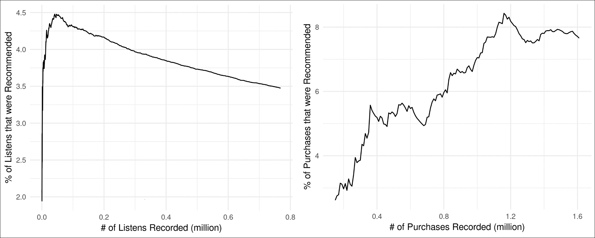
Figure 4: Accuracy of the recommendation system for Last.fm (left) and Amazon (right) datasets
These online evaluation statistics may be generated over time, as purchases occur. Thus, they can be used to provide live, continuous evaluation of the system. In Chapter 3, A Blueprint for Making Sense of Feedback, we developed a live-updating plot of the internet's sentiment about particular topics. We could use the same technology here to show a live-updating plot of the recommendation system's accuracy. Using insights developed in Chapter 6, A Blueprint for Discovering Trends and Recognizing Anomalies, we can then detect anomalies, or sudden changes in accuracy, and throw alerts to figure out what changed in the recommendation system or the data provided to it.