In order to detect which photos on social media have logos and recognize which logos they are, we will develop a series of increasingly sophisticated DL neural networks. Ultimately, we will demonstrate two approaches: one using the Keras library in the TensorFlow platform, and one using YOLO in the Darknet platform. We will write some Python code for the Keras example, and we will use existing open source code for YOLO.

First, we create a straightforward deep network with several convolutional and pooling layers, followed by a fully connected (dense) network. We will use images from the FlickrLogos dataset (Scalable Logo Recognition in Real-World Images, Stefan Romberg, Lluis Garcia Pueyo, Rainer Lienhart, Roelof van Zwol, ACM International Conference on Multimedia Retrieval 2011 (ICMR11), Trento, April 2011, http://www.multimedia-computing.de/flickrlogos/), specifically the version with 32 different kinds of logos. Later, with YOLO, we will use the version with 47 logos. This dataset contains 320 training images (10 examples per logo), and 3,960 testing images (30 per logo plus 3,000 images without logos). This is quite a small number of training photos per logo. Also, note that we do not have any no-logo images for training.

The images are stored in directories named after their respective logos. For example, images with an Adidas logo are in the FlickrLogos-v2/train/classes/jpg/adidas folder. Keras includes a convenient image loading functionality via its ImageDataGenerator and DirectoryIterator classes. Just by organizing the images into these folders, we can avoid all the work of loading images and informing Keras of the class of each image.

We start by importing our libraries and setting up the directory iterator. We indicate the image size we want for our first convolutional layer. Images will be resized as necessary when loaded. We also indicate the number of channels (red, green, blue). These channels are separated before the convolutions operate on the images, so each convolution is only applied to one channel at a time:

import re
import numpy as np
from tensorflow.python.keras.models import Sequential, load_model
from tensorflow.python.keras.layers import Input, Dropout, Flatten, Conv2D, MaxPooling2D, Dense, Activation
from tensorflow.python.keras.preprocessing.image import 
DirectoryIterator, ImageDataGenerator

# all images will be converted to this size
ROWS = 256
COLS = 256
CHANNELS = 3

TRAIN_DIR = '.../FlickrLogos-v2/train/classes/jpg/'

img_generator = ImageDataGenerator() # do not modify images

train_dir_iterator = DirectoryIterator(TRAIN_DIR, img_generator, target_size=(ROWS, COLS), color_mode='rgb', seed=1)

Next, we specify the network's architecture. We specify that we will use a sequential model (that is, not a recurrent model with loops in it), and then proceed to add our layers in order. In the convolutional layers, the first argument (for example, 32) indicates how many different convolutions should be learned (per each of the three channels); the second argument gives the kernel size; the third argument gives the stride; and the fourth argument indicates that we want padding on the image for when the convolutions are applied to the edges. This padding, known as "same," is used to ensure the output image (after being convolved) is the same size as the input (assuming the stride is (1,1)):

model = Sequential()
model.add(Conv2D(32, (3,3), strides=(1,1), padding='same', input_shape=(ROWS, COLS, CHANNELS)))
model.add(Activation('relu'))
model.add(Conv2D(32, (3,3), strides=(1,1), padding='same'))
model.add(Activation('relu'))
model.add(MaxPooling2D(pool_size=(2,2)))
model.add(Conv2D(64, (3,3), strides=(1,1), padding='same'))
model.add(Activation('relu'))
model.add(Conv2D(64, (3,3), strides=(1,1), padding='same'))
model.add(Activation('relu'))
model.add(MaxPooling2D(pool_size=(2,2)))
model.add(Conv2D(128, (3,3), strides=(1,1), padding='same'))
model.add(Activation('relu'))
model.add(Conv2D(128, (3,3), strides=(1,1), padding='same'))
model.add(Activation('relu'))
model.add(MaxPooling2D(pool_size=(2,2)))
model.add(Flatten())
model.add(Dense(64))
model.add(Activation('relu'))
model.add(Dropout(0.5))
model.add(Dense(32)) # i.e., one output neuron per class
model.add(Activation('sigmoid'))

Next, we compile the model and specify that we have binary decisions (yes/no for each of the possible logos) and that we want to use stochastic gradient descent. Different choices for these parameters are beyond the scope of this chapter. We also indicate we want to see accuracy scores as the network learns:

model.compile(loss='binary_crossentropy', optimizer='sgd', metrics=['accuracy'])

We can ask for a summary of the network, which shows the layers and the number of weights that are involved in each layer, plus a total number of weights across the whole network:

model.summary()

This network has about 8.6 million weights (also known as trainable parameters).

Lastly, we run the fit_generator function and feed in our training images. We also specify the number of epochs we want, that is, the number of times to look at all the training images:

model.fit_generator(train_dir_iterator, epochs=20)

But nothing is this easy. Our first network performs very poorly, achieving about 3% precision in recognizing logos. With so few examples per logo (just 10), how could we have expected this to work?

In our second attempt, we will use another feature of the image pre-processing library of Keras. Instead of using a default ImageDataGenerator, we can specify that we want the training images to be modified in various ways, thus producing new training images from the existing ones. We can zoom in/out, rotate, and shear. We'll also rescale the pixel values to values between 0.0 and 1.0 rather than 0 and 255:

img_generator = ImageDataGenerator(rescale=1./255, rotation_range=45, zoom_range=0.5, shear_range=30)

Figure 12 shows an example of a single image undergoing random zooming, rotation, and shearing:

Figure 12: Example of image transformations produced by Keras' ImageDataGenerator; photo from https://www.flickr.com/photos/hellocatfood/9364615943

With this expanded training set, we get a few percent better precision. Still not nearly good enough.

The problem is two-fold: our network is quite shallow, and we do not have nearly enough training examples. Combined, these two problems result in the network being unable to develop useful convolutions, thus unable to develop useful features, to feed into the fully connected network.

We will not be able to obtain more training examples, and it would do us no good to simply increase the complexity and depth of the network without having more training examples to train it.

However, we can make use of a technique known as transfer learning. Suppose we take one of those highly accurate deep networks developed for the ImageNet challenge and trained on millions of photos of everyday objects. Since our task is to detect logos on everyday objects, we can reuse the convolutions learned by these massive networks and just stick a different fully connected network on it. We then train the fully connected network using these convolutions, without updating them. For a little extra boost, we can follow this by training again, this time updating the convolutions and the fully connected network simultaneously. In essence, we'll follow this analogy: grab an existing camera and learn to see through it as best we can; then, adjust the camera a little bit to see even better.

Keras has support for several ImageNet models, shown in the following table (https://keras.io/applications/). Since the Xception model is one of the most accurate but not extremely large, we will use it as a base model:

First, we import the Xception model and remove the top (its fully connected layers), keeping only its convolutional and pooling layers:

from tensorflow.python.keras.applications.xception import Xception

# create the base pre-trained model
base_model = Xception(weights='imagenet', include_top=False, pooling='avg')

Then we create new fully connected layers:

# add some fully-connected layers
dense_layer = Dense(1024, activation='relu')(base_model.output)
out_layer = Dense(32)(dense_layer)
out_layer_activation = Activation('sigmoid')(out_layer)

We put the fully connected layers on top to complete the network:

# this is the model we will train
model = Model(inputs=base_model.input, outputs=out_layer_activation)

Next, we indicate that we don't want the convolutions to change during training:

# first: train only the dense top layers 
# (which were randomly initialized)
# i.e. freeze all convolutional Xception layers
for layer in base_model.layers:
  layer.trainable = False

We then compile the model, print a summary, and train it:

model.compile(loss='categorical_crossentropy', optimizer='sgd', metrics=['accuracy'])

model.summary()

model.fit_generator(train_dir_iterator, epochs=EPOCHS)

Now we're ready to update the convolutions and the fully connected layers simultaneously for that extra little boost in accuracy:

# unfreeze all layers for more training
for layer in model.layers:
  layer.trainable = True

model.compile(loss='categorical_crossentropy', optimizer='sgd', metrics=['accuracy'])

model.fit_generator(train_dir_iterator, epochs=EPOCHS)

We use ImageDataGenerator to split the training data into 80% training examples and 20% validation examples. These validation images allow us to see how well we're doing during training. They simulate what it is like to look at the testing data, that is, photos we have not seen during training.

We can plot the accuracy of logo detection per epoch. Across 400 epochs (200 without updating the convolutions, then another 200 updating the convolutions), we get the plot in Figure 13. Training took a couple hours on an NVIDIA Titan X Pascal, though less powerful GPUs may be used. In some cases, a batch size of 16 or 32 must be specified to indicate how many images to process at once so that the GPU's memory limit is not exceeded. One may also train using no GPU (that is, just the CPU) but this takes considerably longer (like, 10-20x longer).

Interestingly, accuracy on the validation set gets a huge boost when we train the second time and update the convolutions. Eventually, the accuracy of the training set is maximized (nearly 100%) since the network has effectively memorized the training set. This is not necessarily evidence of overfitting, however, since accuracy on the validation set remains relatively constant after a certain point. If we were overfitting, we would see accuracy in the validation set begin to drop:

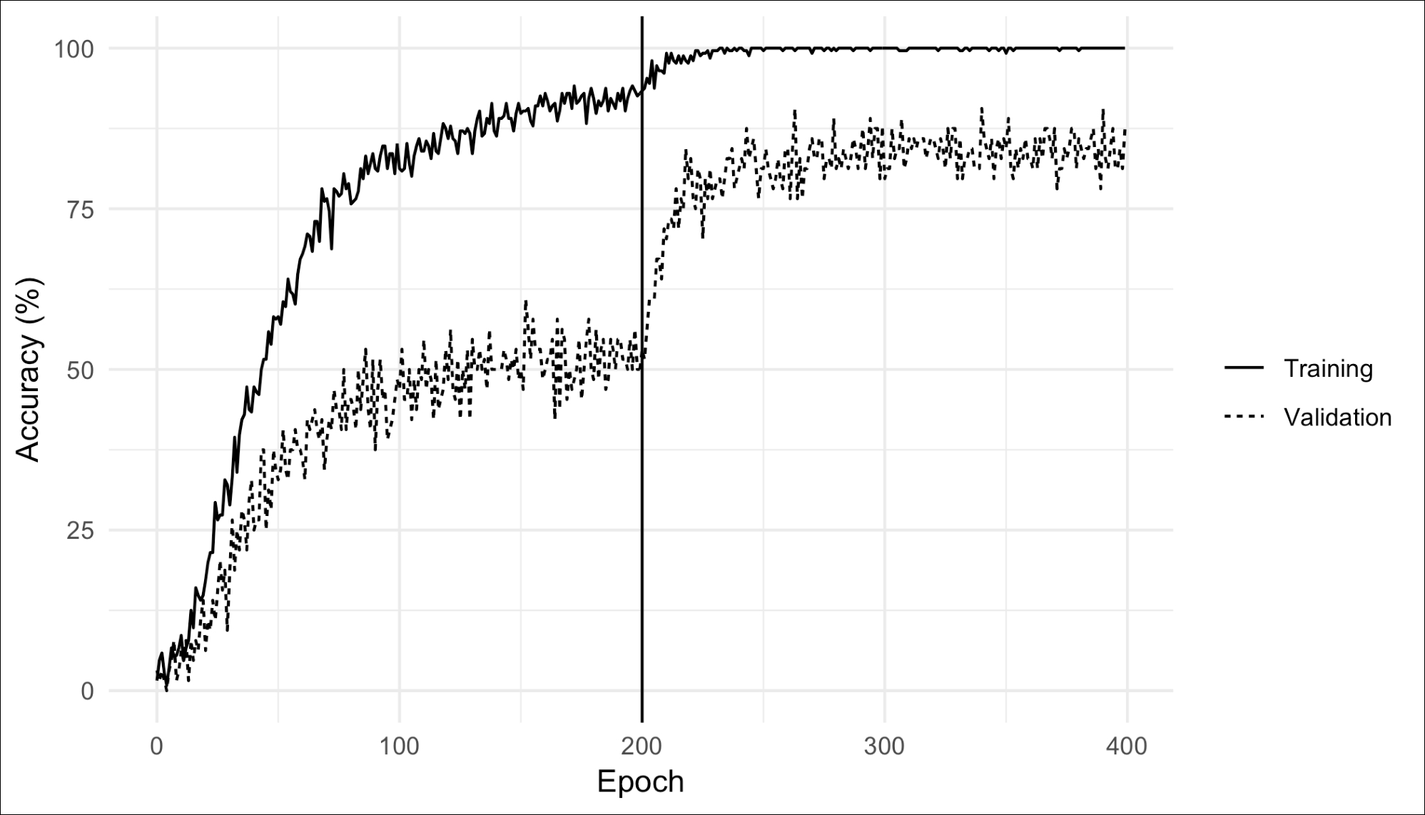
Figure 13: Accuracy over many epochs of our Xception-based model

With this advanced network, we achieve far better accuracy in logo recognition. We have one last issue to solve. Since our training images all had logos, our network is not trained on "no-logo" images. Thus, it will assume every image has a logo, and it is just a matter of figuring out which one. However, the actual situation is that some photos have logos and some do not, so we need to first detect whether there is a logo, and second recognize which logo it is.

We will use a simple detection scheme: if the network is not sufficiently confident about any particular logo (depending on a threshold that we choose), we will say there is no logo. Now that we are able to detect images with logos, we can measure how accurately it recognizes the logo in those images. Our detection threshold influences this accuracy since a high confidence threshold will result in fewer recognized logos, reducing recall. However, a high threshold increases precision since, among those logos it is confident about, it is less likely to be wrong. This tradeoff is often plotted in a precision/recall graph, as shown in Figure 14. Here, we show the impact of different numbers of epochs and different confidence thresholds (the numbers above the lines). The best position to be in is the top-right. Note that the precision scale (y-axis) goes to 1.0 since we are able to achieve high precision, but the recall scale (x-axis) only goes to about 0.40 since we are never able to achieve high recall without disastrous loss of precision. Also note that with more epochs, the output values of the network are smaller (the weights have been adjusted many times, creating a very subtle distinction between different outputs, that is, different logos), so we adjust the confidence threshold lower:

Figure 14: Precision/recall trade-off for logo recognition with our Xception-based model and different numbers of epochs and threshold values

Although our recognition recall value is low (about 40%, meaning we fail to detect logos in 60% of the photos that have logos), our precision is very high (about 90%, meaning we almost always get the right logo when we detect that there is a logo at all).

It is interesting to see how the network mis-identifies logos. We can visualize this with a confusion matrix, which shows the true logo on the left axis and the predicted logo on the bottom axis. In the matrix, a dark blue box indicates the network produces lots of cases of that row/column combination. Figure 15 shows the matrix for our network after 100 epochs. We see that it mostly gets everything right: the diagonal is the darkest blue, in most cases. However, where it gets the logos confused is instructive.

For example, Paulaner and Erdinger are sometimes confused. This makes sense because both logos are circular (one circle inside another) with white text around the edge. Heineken and Becks logos are also sometimes confused. They both have a dark strip in the middle of their logo with white text, and a surrounding oval or rectangular border. NVIDIA and UPS are sometimes confused, though it is not at all obvious why.

Most interestingly, DHL, FedEx, and UPS are sometimes confused. These logos do not appear to have any visual similarities. But we have no reason to believe the neural network, even with all its sophistication and somewhat miraculous accuracy, actually knows anything about logos. Nothing in these algorithms forces it to learn about the logo in each image rather than learn about the image itself. We can imagine that most or all of the photos with DHL, FedEx, or UPS logos have some sort of package, truck, and/or plane in the image as well. Perhaps the network learned that planes go with DHL, packages with FedEx, and trucks with UPS? If this is the case, it will declare (inaccurately) that a photo with a UPS logo on a package is a photo with a FedEx logo, not because it confuses the logos, but because it confuses the rest of the image. This gives evidence that the network has no idea what a logo is. It knows packages, trucks, beer glasses, and so on. Or maybe not. The only way we would be able to tell what it learned is to process images with logos removed and see what it says. We can also visualize some of the convolutions for different images, as we did in Figure 9, though with so many convolutions in the Xception network, this technique will probably provide little insight.

Explaining how a deep neural network does its job, explaining why it arrives at its conclusions, is ongoing active research and currently a big drawback of DL. However, DL is so successful in so many domains that the explainability of it takes a back seat to the performance. MIT's Technology Review addressed this issue in an article written by Will Knight titled, The Dark Secret at the Heart of AI, and subtitled, No one really knows how the most advanced algorithms do what they do. That could be a problem (https://www.technologyreview.com/s/604087/the-dark-secret-at-the-heart-of-ai/).

This issue matters little for logo detection, but the stakes are completely different when DL is used in an autonomous vehicle or medical imaging and diagnosis. In these use cases, if the AI gets it wrong and someone is hurt, it is important that we can determine why and find a solution.

Figure 15: Confusion matrix for a run of our Xception-based model