Example in Computer Graphics
In this chapter, we introduce a simple computer graphics algorithm called marching cubes. The algorithm is a simple but a very data-intensive operation depending on the data set. This chapter also discusses how to implement it in plain MATLAB, how to improve speed performance in MATLAB, and how to accelerate the speed using c-mex and CUDA.
Keywords
Computer graphics algorithm; marching cubes algorithm; isosurface
7.1 Chapter Objectives
In this chapter, we introduce a simple computer graphics algorithm called marching cubes. The algorithm is a simple but very data-intensive operation depending on the data set. In this chapter, we
7.2 Marching Cubes
Marching cubes is a simple yet very powerful computer graphics algorithm that can be used in various applications, especially in 3D visualizations. Given a stack of images, this algorithm extracts a 3D isosurface in the form of triangles, where each point on the surface has the same constant value. Input data can come from various sources, such as CT and MRI scans. They usually come in a stack of 2D images as shown in Figure 7.1. In volume data, each data point is referred to as a voxel. The eight voxels in Figure 7.2 form a cube.


With M×N×P volume data, we have (M−1)×(N−1)×(P−1) cubes in the whole data set. Each vertex of a cube is assigned a voxel value. The value at each vertex could be higher or lower than an isosurface value. The basic idea of the algorithm is to find the points where the isosurface intersect on the cube edges, then construct triangles from those points at intersections. Consider the cube in Figure 7.2 and let us label each vertex and edge. There are eight vertices and 12 edges. We label them as in Figure 7.3. Since each vertex in a cube can be higher or lower than the isosurface value, there are 256 (28) possible cases with 15 unique cases due to symmetry (Figure 7.4).


For simplicity, let us assume our vertex V0 is above the isosurface value and the rest are below it, so that our V0 is an inside object, as shown in Figure 7.5. This falls into the second case on the top in Figure 7.4. In this case, the isosurface crosses three edges: E0, E8 and E3. The intersection points on those edges can be linearly interpolated.

Figure 7.5 The vertex V0 is above the isosurface value.
This results in one triangle with a normal vector.
The isosurface in this cube is then approximated with a triangle with three points. We define the normal vector for this triangle so that it points toward the lower isosurface side. We can work out all other 255 cases and determine all the triangles in each case. This has been worked out already and we can use the predetermined lookup tables for each case.
The algorithm provides two main tables: edge table and triangle table. First, using eight vertexes as 8-bit binary numbers, we determine the cube number:
![]()
In our case, the cube number is 1:

Using this value, we look at the edge table. From the edge table, we get the value, 265. If we convert this to a 12-bit binary number, each bit represents the edge number. It is set to 1 if the isosurface intersects with this edge. In our case,

From the binary values, we now know that the edge, E0, E3, and E8 are the ones that intersect with the isosurface. We can linearly interpolate where on those edges the surface intersects. For instance, the intersection point on E3 can be estimated as
![]()
where I0 and I3 are intensity values at vertex V0 and V3, respectively.
Then, the second table gives indexes of a triangle in order. This enables us to determine in which direction the normal vector goes or which side faces outward. For our cube, the triangle table gives
0, 8, 3, −1, −1, −1, −1, −1, −1, −1, −1, −1, −1, −1, −1, −1
As per the table, the triangle is defined by points on E0, E8, and E3, in that order. The lookup tables in Figure 7.6 make it easy to find out all the possible triangles and their indexes.

7.3 Implementation in MATLAB
This section shows how to implement the marching cubes algorithm in MATLAB. We first do the straight implementation of the algorithm in MATLAB to demonstrate the algorithm itself. In this implementation, we visit each voxel and determine the triangles. The full implementation can be found in testSurfaceNoOpt.m and getSurfaceNoOpt.m or at the end of the steps.
7.3.1 Step 1
First, let us generate a small sample of volume data using the MATLAB command, flow. In the MATLAB command window, enter the following:
% generate sample volume data
[X, Y, Z, V] = flow;
% visualize volume data
figure
xmin = min(X(:));
ymin = min(Y(:));
zmin = min(Z(:));
xmax = max(X(:));
ymax = max(Y(:));
zmax = max(Z(:));
hslice=surf(linspace(xmin,xmax,100), linspace(ymin,ymax,100), zeros(100));
rotate(hslice,[-1,0,0],-45)
xd = get(hslice,'XData'),
yd = get(hslice,'YData'),
zd = get(hslice,'ZData'),
delete(hslice)
h = slice(X,Y,Z,V,xd,yd,zd);
set(h,'FaceColor', 'interp', 'EdgeColor', 'none', 'DiffuseStrength', 0.8)
hold on
hx = slice(X,Y,Z,V,xmax,[],[]);
set(hx,'FaceColor', 'interp', 'EdgeColor', 'none')
hy = slice(X,Y,Z,V,[],ymax,[]);
set(hy,'FaceColor', 'interp', 'EdgeColor', 'none')
hz = slice(X,Y,Z,V,[],[],zmin);
set(hz,'FaceColor', 'interp', 'EdgeColor', 'none')
By default, this generates four variables: X, Y, Z, and V. They are 25×50×25 matrices that contain the positions and intensities at voxels. The rest of the lines let you visualize data. If you execute the code now, this volume data will look like Figure 7.7.

If you wish, further explore visualization options from MATLAB Help in MATLAB>User’s Guide>3-D Visualization>Volume Visualization Techniques>Exploring Volumes with Slice Planes. We later find the size of the volume data along X, Y, and Z and define our isovalue to be −3.
7.3.2 Step 2
We then define a function to perform the marching cubes algorithm and save it as getSurfaceNoOpt.m. This function gets five inputs and returns two outputs that contain all the vertexes and indexes of the triangles we find in the volume data. We show only partial table values. The full table values can be found in the provided getSurfaceNoOpt.m file.
function [Vertices, Indices] = getSurfaceNoOpt(X, Y, Z, V, isovalue)
edgeTable = uint16([
0, 265, 515, 778, 1030, 1295, 1541, 1804, …
2060, 2309, 2575, 2822, 3082, 3331, 3593, 3840, …
…
…
1804, 1541, 1295, 1030, 778, 515, 265, 0]);
triTable = [
−1, −1, −1, −1, −1, −1, −1, −1, −1, −1, −1, −1, −1, −1, −1, −1;
0, 8, 3, −1, −1, −1, −1, −1, −1, −1, −1, −1, −1, −1, −1, −1;
…
…
−1, −1, −1, −1, −1, −1, −1, −1, −1, −1, −1, −1, −1, −1, −1, −1];
sizeX = size(V, 1);
sizeY = size(V, 2);
sizeZ = size(V, 3);
MAX_VERTICES = 15;
% vertices and indices
VertexBin = single(zeros(sizeX, sizeY, sizeZ, MAX_VERTICES, 3));
TriCounter = zeros(sizeX, sizeY, sizeZ);
totalTriangles = 0;
We first create two precalculated lookup tables for the marching cubes algorithm. Next, we determine sizes of the volume in the x, y, and z directions. Then, we preallocate temporary variables for all of our vertex and index storages.
7.3.3 Step 3
In this step, we march through all the cubes in the volume data. We visit every cube in nested loops. If the volume data size is M×N×P, then there will be (M−1)×(N−1)×(P−1) cubes in all.
for k = 1:sizeZ - 1
for j = 1:sizeY - 1
for i = 1:sizeX - 1
…
% algorithm goes in here
…
end
end
end
7.3.4 Step 4
In the innermost loop, we read the intensity values and positions at eight vertexes of the cube we are processing. They are assigned according to the vertex labels in Figure 7.3.
% temp. vars for voxels and isopoints.
voxels = single(zeros(8, 4)); %[v, x, y, z]
isoPos = single(zeros(12, 3)); %[x, y, z]
%cube
voxels(1,:)=[V(i, j, k), X(i, j, k), Y(i, j, k), Z(i, j, k)];
voxels(2,:)=[V(i, j+1, k), X(i, j+1, k), Y(i, j+1, k), Z(i, j+1, k)];
voxels(3,:)=[V(i+1, j+1, k), X(i+1, j+1, k), Y(i+1, j+1, k), Z(i+1, j+1, k)];
voxels(4,:)=[V(i+1, j, k), X(i+1, j, k), Y(i+1, j, k), Z(i+1, j, k)];
voxels(5,:)=[V(i, j, k+1), X(i, j, k+1), Y(i, j, k+1), Z(i, j, k+1)];
voxels(6,:)=[V(i, j+1, k+1), X(i, j+1, k+1), Y(i, j+1, k+1), Z(i, j+1, k+1)];
voxels(7,:)=[V(i+1, j+1, k+1), X(i+1, j+1, k+1), Y(i+1, j+1,k+1), Z(i+1, j+1, k+1)];
voxels(8,:)=[V(i+1, j, k+1), X(i+1, j, k+1), Y(i+1, j, k+1), Z(i+1, j, k+1)];
7.3.5 Step 5
We check the intensity value at each vertex to see if it is above or below the isovalue. A bit position for a vertex is set if the value is above the isovalue. Since we have eight vertexes, there are 256 cases in total. After checking all the values at the eight vertexes, we determine the cube index. We use this cube index to get the edge values from the edge table.
% find the cube index
cubeIndex = uint16(0);
for n = 1:8
>if voxels(n, 1) >= isovalue
>cubeIndex = bitset(cubeIndex, n);
>end
end
cubeIndex = cubeIndex + 1;
% get edges from edgeTable
edges = edgeTable(cubeIndex);
if edges==0
continue;
end
7.3.6 Step 6
After getting the edge values from the edge table, we locate the edges on which the isosurface intersects and find the intersection points on those edges. We first create a new function for the interpolation. This function receives two voxels and isovalues as input and outputs the interpolated position.
function [varargout] = interpolatePos(isovalue, voxel1, voxel2)
scale = (isovalue−voxel1(:,1)) ./ (voxel2(:,1)−voxel1(:,1));0
interpolatedPos=voxel1(:,2:4)+[scale .* (voxel2(:,2)−voxel1(:,2)), …
scale .* (voxel2(:,3)−voxel1(:,3)), …
scale .* (voxel2(:,4)−voxel1(:,4))];
if nargout==1 || nargout==0
varargout{1}=interpolatedPos;
elseif nargout==3
varargout{1}=interpolatedPos(:,1);
varargout{2}=interpolatedPos(:,2);
varargout{3}=interpolatedPos(:,3);
end
Going back to our main function code, we continue checking the edges and call the interpolation function for each edge, if applicable:
% check 12 edges
if bitand(edges, 1)
isoPos(1,:) = interpolatePos(isovalue, voxels(1,:), voxels(2,:));
end
if bitand(edges, 2)
isoPos(2,:) = interpolatePos(isovalue, voxels(2,:), voxels(3,:));
end
if bitand(edges, 4)
isoPos(3,:) = interpolatePos(isovalue, voxels(3,:), voxels(4,:));
end
if bitand(edges, 8)
isoPos(4,:) = interpolatePos(isovalue, voxels(4,:), voxels(1,:));
end
if bitand(edges, 16)
isoPos(5,:) = interpolatePos(isovalue, voxels(5,:), voxels(6,:));
end
if bitand(edges, 32)
isoPos(6,:) = interpolatePos(isovalue, voxels(6,:), voxels(7,:));
end
if bitand(edges, 64)
isoPos(7,:) = interpolatePos(isovalue, voxels(7,:), voxels(8,:));
end
if bitand(edges, 128)
isoPos(8,:) = interpolatePos(isovalue, voxels(8,:), voxels(5,:));
end
if bitand(edges, 256)
isoPos(9,:) = interpolatePos(isovalue, voxels(1,:), voxels(5,:));
end
if bitand(edges, 512)
isoPos(10,:) = interpolatePos(isovalue, voxels(2,:), voxels(6,:));
end
if bitand(edges, 1024)
isoPos(11,:) = interpolatePos(isovalue, voxels(3,:), voxels(7,:));
end
if bitand(edges, 2048)
isoPos(12,:) = interpolatePos(isovalue, voxels(4,:), voxels(8,:));
end
7.3.7 Step 7
From the triangle table, we find out how many triangles there are and their indexes. We go through the predetermined vertex order from the triangle table and register all the triangles we identify. There can be five triangles at maximum.
%walk through the triTable and get the triangle(s) vertices
numTriangles = 0;
numVertices = 0;
for n = 1:3:16
if triTable(cubeIndex, n) < 0
break;
end
% first vertex
numVertices = numVertices + 1;
edgeIndex = triTable(cubeIndex, n) + 1;
vertexBin(i, j, k, numVertices, :) = isoPos(edgeIndex, :);
% second vertex
numVertices = numVertices + 1;
edgeIndex = triTable(cubeIndex, n + 1) + 1;
vertexBin(i, j, k, numVertices, :) = isoPos(edgeIndex, :);
% third vertex
numVertices = numVertices + 1;
edgeIndex = triTable(cubeIndex, n + 2) + 1;
vertexBin(i, j, k, numVertices, :) = isoPos(edgeIndex, :);
numTriangles = numTriangles + 1;
end
TriCounter(i, j, k) = numTriangles;
totalTriangels = totalTriangles + numTriangles;
7.3.8 Step 8
After we find all the triangles in a cube, we add them to our output storages for vertexes and indexes:
Vertices = single(zeros(totalTriangles * 3, 3));
Indices = uint32(zeros(totalTriangels, 3));
vIdx = 0;
tIdx = 0;
for k = 1:sizeZ - 1
for j = 1:sizeY - 1
for i = 1:sizeX - 1
count = TriCounter(i, j, k);
if count < 1
continue;
end
for t = 0:count - 1
vIdx = vIdx + 1;
Vertices(vIdx, :) = vertexBin(i, j, k, 3*t + 1, :);
vIdx = vIdx + 1;
Vertices(vIdx, :) = vertexBin(i, j, k, 3*t + 2, :);
vIdx = vIdx + 1;
Vertices(vIdx, :) = vertexBin(i, j, k, 3*t + 3, :);
tIdx = tIdx + 1;
Indices(tIdx, :)=uint32([3 * tIdx−2, 3 * tIdx−1, 3 * tIdx]);
end
end
end
end
7.3.9 Step 9
After we calculate all the vertexes and triangle indexes, we can visualize the triangles as follows. Back in testSurfaceNoOpt.m, append the following lines for triangle visualization:
% data type to single
X = single(X);
Y = single(Y);
Z = single(Z);
V = single(V);
isovalue = single(-3);
% Marching cubes
[Vertices1, Indices1] = getSurfaceNoOpt(X, Y, Z, V, isovalue);
% visualize triangles
figure
p = patch('Faces', Indices1, 'Vertices', Vertices1);
set(p, 'FaceColor', 'none', 'EdgeColor', 'red'),
daspect([1,1,1])
view(3);
camlight
lighting gouraud
grid on
The triangles we found using marching cubes are now shown in Figure 7.8.

The following is the full implementation in MATLAB, including two lookup tables. Note that there are duplicate vertexes in our final vertex results. One go on to remove those duplicate vertexes, thus reducing our final storage size. However, we stop here without further reducing the duplicates for the purpose of demonstrating the algorithm.
Here are the full codes in three files. The table values shown are truncated. The full table values can be found in the provided getSurfaceNoOpt.m file.
getSurfaceNoOpt.m
function [Vertices, Indices] = getSurfaceNoOpt(X, Y, Z, V, isovalue)
edgeTable = uint16([
0, 265, 515, 778, 1030, 1295, 1541, 1804, …
2060, 2309, 2575, 2822, 3082, 3331, 3593, 3840, …
400, 153, 915, 666, 1430, 1183, 1941, 1692, …
2460, 2197, 2975, 2710, 3482, 3219, 3993, 3728, …
560, 825, 51, 314, 1590, 1855, 1077, 1340, …
…
…
…
3728, 3993, 3219, 3482, 2710, 2975, 2197, 2460, …
1692, 1941, 1183, 1430, 666, 915, 153, 400, …
3840, 3593, 3331, 3082, 2822, 2575, 2309, 2060, …
1804, 1541, 1295, 1030, 778, 515, 265, 0]);
triTable = [
−1, −1, −1, −1, −1, −1, −1, −1, −1, −1, −1, −1, −1, −1, −1, −1;
0, 8, 3, −1, −1, −1, −1, −1, −1, −1, −1, −1, −1, −1, −1, −1;
0, 1, 9, −1, −1, −1, −1, −1, −1, −1, −1, −1, −1, −1, −1, −1;
1, 8, 3, 9, 8, 1, −1, −1, −1, −1, −1, −1, −1, −1, −1, −1;
…
…
…
1, 3, 8, 9, 1, 8, −1, −1, −1, −1, −1, −1, −1, −1, −1, −1;
0, 9, 1, −1, −1, −1, −1, −1, −1, −1, −1, −1, −1, −1, −1, −1;
0, 3, 8, −1, −1, −1, −1, −1, −1, −1, −1, −1, −1, −1, −1, −1;
−1, −1, −1, −1, −1, −1, −1, −1, −1, −1, −1, −1, −1, −1, −1, −1];
sizeX = size(V, 1);
sizeY = size(V, 2);
sizeZ = size(V, 3);
MAX_VERTICES = 15;
% vertices and indices
VertexBin = single(zeros(sizeX, sizeY, sizeZ, MAX_VERTICES, 3));
TriCounter = zeros(sizeX, sizeY, sizeZ);
totalTriangles = 0;
% marching through the cubes
for k = 1:sizeZ - 1
for j = 1:sizeY - 1
for i = 1:sizeX - 1
% temp. vars for voxels and isopoints.
voxels = single(zeros(8, 4)); %[v, x, y, z]
isoPos = single(zeros(12, 3)); %[x, y, z]
%cube
voxels(1,:)=[V(i, j, k), X(i, j, k), Y(i, j, k), Z(i, j, k)];
voxels(2,:)=[V(i, j+1,k), X(i, j+1,k), Y(i, j+1,k), Z(i, j+1,k)];
voxels(3,:)=[V(i+1,j+1,k), X(i+1,j+1,k), Y(i+1,j+1,k), Z(i+1,j+1,k)];
voxels(4,:)=[V(i+1,j, k), X(i+1,j, k), Y(i+1,j, k), Z(i+1,j, k)];
voxels(5,:)=[V(i, j, k+1),X(i, j, k+1),Y(i, j, k+1),Z(i, j, k+1)];
voxels(6,:)=[V(i, j+1,k+1),X(i, j+1,k+1),Y(i, j+1,k+1),Z(i, j+1,k+1)];
voxels(7,:)=[V(i+1,j+1,k+1),X(i+1,j+1,k+1),Y(i+1,j+1,k+1),Z(i+1,j+1,k+1)];
voxels(8,:)=[V(i+1,j, k+1),X(i+1,j, k+1),Y(i+1,j, k+1),Z(i+1,j, k+1)];
% find the cube index
cubeIndex = uint16(0);
for n = 1:8
if voxels(n, 1) >= isovalue
cubeIndex = bitset(cubeIndex, n);
end
end
cubeIndex = cubeIndex + 1;
% get edges from edgeTable
edges = edgeTable(cubeIndex);
if edges == 0
continue;
end
% check 12 edges
if bitand(edges, 1)
isoPos(1,:) = interpolatePos(isovalue, voxels(1,:), voxels(2,:));
end
if bitand(edges, 2)
isoPos(2,:) = interpolatePos(isovalue, voxels(2,:), voxels(3,:));
end
if bitand(edges, 4)
isoPos(3,:) = interpolatePos(isovalue, voxels(3,:), voxels(4,:));
end
if bitand(edges, 8)
isoPos(4,:) = interpolatePos(isovalue, voxels(4,:), voxels(1,:));
end
if bitand(edges, 16)
isoPos(5,:) = interpolatePos(isovalue, voxels(5,:), voxels(6,:));
end
if bitand(edges, 32)
isoPos(6,:) = interpolatePos(isovalue, voxels(6,:), voxels(7,:));
end
if bitand(edges, 64)
isoPos(7,:) = interpolatePos(isovalue, voxels(7,:), voxels(8,:));
end
if bitand(edges, 128)
isoPos(8,:) = interpolatePos(isovalue, voxels(8,:), voxels(5,:));
end
if bitand(edges, 256)
isoPos(9,:) = interpolatePos(isovalue, voxels(1,:), voxels(5,:));
end
if bitand(edges, 512)
isoPos(10,:) = interpolatePos(isovalue, voxels(2,:), voxels(6,:));
end
if bitand(edges, 1024)
isoPos(11,:) = interpolatePos(isovalue, voxels(3,:), voxels(7,:));
end
if bitand(edges, 2048)
isoPos(12,:) = interpolatePos(isovalue, voxels(4,:), voxels(8,:));
end
%walk through the triTable and get the triangle(s) vertices
numTriangles = 0;
numVertices = 0;
for n = 1:3:16
if triTable(cubeIndex, n) < 0
break;
end
% first vertex
numVertices = numVertices + 1;
edgeIndex = triTable(cubeIndex, n) + 1;
vertexBin(i, j, k, numVertices, :) = isoPos(edgeIndex, :);
% second vertex
numVertices = numVertices + 1;
edgeIndex = triTable(cubeIndex, n + 1) + 1;
vertexBin(i, j, k, numVertices, :) = isoPos(edgeIndex, :);
% third vertex
numVertices = numVertices + 1;
edgeIndex = triTable(cubeIndex, n + 2) + 1;
vertexBin(i, j, k, numVertices, :) = isoPos(edgeIndex, :);
numTriangles = numTriangles + 1;
end
TriCounter(i, j, k) = numTriangles;
totalTriangels = totalTriangles + numTriangles;
end
end
end
Vertices = single(zeros(totalTriangles * 3, 3));
Indices = uint32(zeros(totalTriangels, 3));
vIdx = 0;
tIdx = 0;
for k = 1:sizeZ - 1
for j = 1:sizeY - 1
for i = 1:sizeX - 1
count = TriCounter(i, j, k);
if count < 1
continue;
end
for t = 0:count - 1
vIdx = vIdx + 1;
Vertices(vIdx, :) = vertexBin(i, j, k, 3*t + 1, :);
vIdx = vIdx + 1;
Vertices(vIdx, :) = vertexBin(i, j, k, 3*t + 2, :);
vIdx = vIdx + 1;
Vertices(vIdx, :) = vertexBin(i, j, k, 3*t + 3, :);
tIdx = tIdx + 1;
Indices(tIdx, :) = uint32([3 * tIdx - 2, 3 * tIdx - 1, 3 * tIdx]);
end
end
end
end
InterpolatePos.m
function [varargout] = interpolatePos(isovalue, voxel1, voxel2)
scale = (isovalue - voxel1(:,1)) ./ (voxel2(:,1) - voxel1(:,1));
interpolatedPos=voxel1(:,2:4)+[scale .* (voxel2(:,2)−voxel1(:,2)), …
scale .* (voxel2(:,3)−voxel1(:,3)), …
scale .* (voxel2(:,4) - voxel1(:,4))];
if nargout == 1 || nargout == 0
varargout{1} = interpolatedPos;
elseif nargout == 3
varargout{1} = interpolatedPos(:,1);
varargout{2} = interpolatedPos(:,2);
varargout{3} = interpolatedPos(:,3);
end
testSurfaceNoOpt.m
% generate sample volume data
[X, Y, Z, V] = flow;
% visualize volume data
figure
xmin = min(X(:));
ymin = min(Y(:));
zmin = min(Z(:));
xmax = max(X(:));
ymax = max(Y(:));
zmax = max(Z(:));
hslice = surf(linspace(xmin,xmax,100), linspace(ymin,ymax,100), zeros(100));
rotate(hslice,[-1,0,0],-45)
xd = get(hslice,'XData'),
yd = get(hslice,'YData'),
zd = get(hslice,'ZData'),
delete(hslice)
h = slice(X,Y,Z,V,xd,yd,zd);
set(h,'FaceColor', 'interp', 'EdgeColor', 'none', 'DiffuseStrength', 0.8)
hold on
hx = slice(X,Y,Z,V,xmax,[],[]);
set(hx,'FaceColor', 'interp', 'EdgeColor', 'none')
hy = slice(X,Y,Z,V,[],ymax,[]);
set(hy,'FaceColor', 'interp', 'EdgeColor', 'none')
hz = slice(X,Y,Z,V,[],[],zmin);
set(hz,'FaceColor', 'interp', 'EdgeColor', 'none')
% data type to single
X = single(X);
Y = single(Y);
Z = single(Z);
V = single(V);
isovalue = single(-3);
% Marching cubes
[Vertices1, Indices1] = getSurfaceNoOpt(X, Y, Z, V, isovalue);
% visualize triangles
figure
p = patch('Faces', Indices1, 'Vertices', Vertices1);
set(p, 'FaceColor', 'none', 'EdgeColor', 'red'),
daspect([1,1,1])
view(3);
camlight
lighting gouraud
7.3.10 Time Profiling
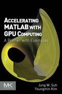
Now, we can profile our implementation using Profiler in MATLAB. Open Profiler by pressing Ctrl+5 or selecting Windows>5 Profiler from the main MATLAB menu. Then, enter the MATLAB code file name and run it. We get the profile summary in Figure 7.9.
Overall, our performance took about 1.9 seconds in total. If we click on the getSurfaceNoOpt link in the summary, we see more detailed results (Figure 7.10).

According to our profiler results, we spent most of the time assigning empty voxels and finding out the cube index.
7.4 Implementation in c-mex with CUDA
With a straightforward implementation of the marching cubes algorithm, we got about 1.9 seconds of time performance. In this section, we will go show how we can improve our implementation using only MATLAB codes. We will use the concept of vectorization and preallocation introduced in Chapter 1. Our strategy will be, instead of visiting each and every voxel, we preallocate temporary storages for storing intermediate results and try to calculate the triangles without introducing triple for-loops.
7.4.1 Step 1
Create a new function, getSurfaceWithOpt, type in the code follows, and save it as getSurfaceWithOpt.m.
getSurfaceWithOpt.m
function [Vertices, Indices] = getSurfaceWithOpt(X, Y, Z, V, isovalue)
edgeTable = uint16([
0, 265, 515, 778, 1030, 1295, 1541, 1804, …
2060, 2309, 2575, 2822, 3082, 3331, 3593, 3840, …
…
…
1804, 1541, 1295, 1030, 778, 515, 265, 0]);
triTable = [
−1, −1, −1, −1, −1, −1, −1, −1, −1, −1, −1, −1, −1, −1, −1, −1;
0,8,3, −1, −1, −1, −1, −1, −1, −1, −1, −1, −1, −1, −1, −1;
…
…
−1, −1, −1, −1, −1, −1, −1, −1, −1, −1, −1, −1, −1, −1, −1, −1];
sx = size(V, 1);
sy = size(V, 2);
sz = size(V, 3);
% Cube Index
CV = uint16(V > isovalue);
Cubes = zeros(sx−1, sy-1, sz-1, 'uint16'),
Cubes = Cubes + CV(1:sx-1, 1:sy-1, 1:sz-1);
Cubes = Cubes + CV(1:sx-1, 2:sy, 1:sz-1) * 2;
Cubes = Cubes + CV(2:sx, 2:sy, 1:sz-1) * 4;
Cubes = Cubes + CV(2:sx, 1:sy-1, 1:sz-1) * 8;
Cubes = Cubes + CV(1:sx-1, 1:sy-1, 2:sz) * 16;
Cubes = Cubes + CV(1:sx-1, 2:sy, 2:sz) * 32;
Cubes = Cubes + CV(2:sx, 2:sy, 2:sz) * 64;
Cubes = Cubes + CV(2:sx, 1:sy-1, 2:sz) * 128;
Cubes = Cubes + 1;
% Edges
Edges = edgeTable(Cubes);
EdgeIdx = find(Edges > 0);
EdgeVal = Edges(EdgeIdx);
% Vertices with edges
[vdx, vdy, vdz] = ind2sub(size(Edges), EdgeIdx);
idx = sub2ind(size(X), vdx, vdy, vdz);
Vt1 = [V(idx), X(idx), Y(idx), Z(idx)];
idx = sub2ind(size(X), vdx, vdy+1, vdz);
Vt2 = [V(idx), X(idx), Y(idx), Z(idx)];
idx = sub2ind(size(X), vdx+1, vdy+1, vdz);
Vt3 = [V(idx), X(idx), Y(idx), Z(idx)];
idx = sub2ind(size(X), vdx+1, vdy, vdz);
Vt4 = [V(idx), X(idx), Y(idx), Z(idx)];
idx = sub2ind(size(X), vdx, vdy, vdz+1);
Vt5 = [V(idx), X(idx), Y(idx), Z(idx)];
idx = sub2ind(size(X), vdx, vdy+1, vdz+1);
Vt6 = [V(idx), X(idx), Y(idx), Z(idx)];
idx = sub2ind(size(X), vdx+1, vdy+1, vdz+1);
Vt7 = [V(idx), X(idx), Y(idx), Z(idx)];
idx = sub2ind(size(X), vdx+1, vdy, vdz+1);
Vt8 = [V(idx), X(idx), Y(idx), Z(idx)];
% EdgeNumber
PosX = zeros(size(EdgeVal,1), 12, 'single'),
PosY = zeros(size(EdgeVal,1), 12, 'single'),
PosZ = zeros(size(EdgeVal,1), 12, 'single'),
idx = find(uint16(bitand(EdgeVal, 1)));
[PosX(idx,1), PosY(idx,1), PosZ(idx,1)] = interpolatePos(isovalue, Vt1(idx,:), Vt2(idx,:));
idx = find(uint16(bitand(EdgeVal, 2)));
[PosX(idx,2), PosY(idx,2), PosZ(idx,2)] = interpolatePos(isovalue, Vt2(idx,:), Vt3(idx,:));
idx = find(uint16(bitand(EdgeVal, 4)));
[PosX(idx,3), PosY(idx,3), PosZ(idx,3)] = interpolatePos(isovalue, Vt3(idx,:), Vt4(idx,:));
idx = find(uint16(bitand(EdgeVal, 8)));
[PosX(idx,4), PosY(idx,4), PosZ(idx,4)] = interpolatePos(isovalue, Vt4(idx,:), Vt1(idx,:));
idx = find(uint16(bitand(EdgeVal, 16)));
[PosX(idx,5), PosY(idx,5), PosZ(idx,5)] = interpolatePos(isovalue, Vt5(idx,:), Vt6(idx,:));
idx = find(uint16(bitand(EdgeVal, 32)));
[PosX(idx,6), PosY(idx,6), PosZ(idx,6)] = interpolatePos(isovalue, Vt6(idx,:), Vt7(idx,:));
idx = find(uint16(bitand(EdgeVal, 64)));
[PosX(idx,7), PosY(idx,7), PosZ(idx,7)] = interpolatePos(isovalue, Vt7(idx,:), Vt8(idx,:));
idx = find(uint16(bitand(EdgeVal, 128)));
[PosX(idx,8), PosY(idx,8), PosZ(idx,8)] = interpolatePos(isovalue, Vt8(idx,:), Vt5(idx,:));
idx = find(uint16(bitand(EdgeVal, 256)));
[PosX(idx,9), PosY(idx,9), PosZ(idx,9)] = interpolatePos(isovalue, Vt1(idx,:), Vt5(idx,:));
idx = find(uint16(bitand(EdgeVal, 512)));
[PosX(idx,10), PosY(idx,10), PosZ(idx,10)] = interpolatePos(isovalue, Vt2(idx,:), Vt6(idx,:));
idx = find(uint16(bitand(EdgeVal, 1024)));
[PosX(idx,11), PosY(idx,11), PosZ(idx,11)] = interpolatePos(isovalue, Vt3(idx,:), Vt7(idx,:));
idx = find(uint16(bitand(EdgeVal, 2048)));
[PosX(idx,12), PosY(idx,12), PosZ(idx,12)] = interpolatePos(isovalue, Vt4(idx,:), Vt8(idx,:));
% Triangles
Vertices = zeros(0, 3, 'single'),
TriVal = triTable(Cubes(EdgeIdx),:) + 1;
for i = 1:3:15
idx = find(TriVal(:,i) > 0);
if isempty(idx)
continue;
end
TriVtx = TriVal(idx, i:i+2);
vx1 = PosX(sub2ind(size(PosX), idx, TriVtx(:,1)));
vy1 = PosY(sub2ind(size(PosY), idx, TriVtx(:,1)));
vz1 = PosZ(sub2ind(size(PosZ), idx, TriVtx(:,1)));
vx2 = PosX(sub2ind(size(PosX), idx, TriVtx(:,2)));
vy2 = PosY(sub2ind(size(PosY), idx, TriVtx(:,2)));
vz2 = PosZ(sub2ind(size(PosZ), idx, TriVtx(:,2)));
vx3 = PosX(sub2ind(size(PosX), idx, TriVtx(:,3)));
vy3 = PosY(sub2ind(size(PosY), idx, TriVtx(:,3)));
vz3 = PosZ(sub2ind(size(PosZ), idx, TriVtx(:,3)));
vsz = 3 * size(vx1, 1);
t1 = zeros(vsz, 3, 'single'),
t1(1:3:vsz,:) = [vx1 vy1 vz1];
t1(2:3:vsz,:) = [vx2 vy2 vz2];
t1(3:3:vsz,:) = [vx3 vy3 vz3];
Vertices = [Vertices; t1];
end
Indices = reshape(1:size(Vertices,1), 3, size(Vertices,1)/3)';
In this code, we do have no nested for-loops. Instead, we calculate all the indexes and vertexes as a whole volume. This comes at the cost of more memory space for temporary variables. As the size of volume data grows, this technique might not become feasible. Anyway, if we execute this code, we will be surprised how much time we are able to save.
7.4.2 Step 2
Modify the testSurfaceNoOpt.m file, which follows, and save it as testSurfaceWithOpt.m:
testSurfaceWithOpt.m
% generate sample volume data
[X, Y, Z, V] = flow;
X = single(X);
Y = single(Y);
Z = single(Z);
V = single(V);
isovalue = single(-3);
[Vertices2, Indices2] = getSurfaceWithOpt(X, Y, Z, V, isovalue);
% visualize triangles
figure
p = patch('Faces', Indices2, 'Vertices', Vertices2);
set(p, 'FaceColor', 'none', 'EdgeColor', 'green'),
daspect([1,1,1])
view(3);
camlight
lighting gouraud
grid on
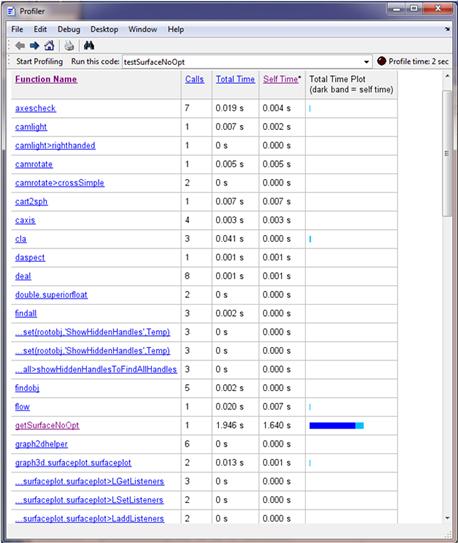
After running this script, we get the same output data with the exception that the triangles are saved in a different order. But, we basically have the same triangles as before (Figure 7.11).
7.4.3 Time Profiling
Let us now perform time profiling on this new, optimized code. Go back to the Profiler and run testSurfaceWithOpt.m (Figure 7.12).

This time, the new function, getSurfaceWithOpt, took only 0.029 seconds, compared to 1.9 seconds with no optimization. This is huge improvement over the straightforward implementation. We saved most of the time by getting rid of triple nested for-loops.
7.5 Implementation Using c-mex and GPU
Without even introducing GPU and c-mex, we can gain huge improvement in speed if we carefully design using vectorization and preallocation techniques, as we have seen in the previous sections. In this section, we further explore how much speed we can squeeze out if we use c-mex and the GPU in our implementation. Overall, we follow our first implementation with no optimization and replace all the operations in the innermost loops with CUDA functions.
7.5.1 Step 1
Create a gateway routine for the c-mex function and fill the main function body as follows. We save this as getSurfaceCuda.cpp.
getSurfaceCuda.cpp
#include "mex.h"
#include <vector>
#include <cuda_runtime.h>
#include "MarchingCubes.h"
// [Vertices, Indices] = getSurface(X, Y, Z, V, isovalue)
void mexFunction(int nlhs, mxArray *plhs[], int nrhs, const mxArray *prhs[])
{
if (nrhs != 5)
mexErrMsgTxt("Invaid number of input arguments");
if (nlhs != 2)
mexErrMsgTxt("Invalid number of outputs");
if (!mxIsSingle(prhs[0]) && !mxIsSingle(prhs[1]) &&
!mxIsSingle(prhs[2]) && !mxIsSingle(prhs[3]) &&
!mxIsSingle(prhs[4]))
mexErrMsgTxt("input vector data type must be single");
const mwSize* size = mxGetDimensions(prhs[3]);
int sizeX = size[0];
int sizeY = size[1];
int sizeZ = size[2];
float* X = (float*mxGetData(prhs[0]);
float*Y = (float*mxGetData(prhs[1]);
float*Z = (float*mxGetData(prhs[2]);
float*V = (float*mxGetData(prhs[3]);
float isovalue = *float*mxGetData(prhs[4]));
float*vertices[3];
unsigned int*indices[3];
int numVertices = 0;
int numTriangles = 0;
marchingCubes(isovalue,
X, Y, Z, V,
sizeX, sizeY, sizeZ,
vertices, indices,
numVertices, numTriangles);
cudaError_t error = cudaGetLastError();
if (error != cudaSuccess)
{
  mexPrintf("%s
", cudaGetErrorString(error));
  mexErrMsgTxt("CUDA failed
");
}
 mexPrintf("numVertices = %d
", numVertices);
 mexPrintf("numTriangles = %d
", numTriangles);
plhs[0]=mxCreateNumericMatrix(numVertices, 3, mxSINGLE_CLASS, mxREAL);
plhs[1]=mxCreateNumericMatrix(numTriangles, 3, mxUINT32_CLASS, mxREAL);
float*Vertices = (float*mxGetData(plhs[0]);
unsigned int*Indices = (unsigned int*mxGetData(plhs[1]);
for (int i = 0; i < 3; ++i)
{
memcpy(Vertices + i *numVertices, vertices[i], numVertices *sizeof(float));
free(vertices[i]);
}
for (int i = 0; i < 3; ++i)
{
memcpy(Indices + i *numTriangles, indices[i], numTriangles *sizeof(unsigned int));
free(indices[i]);
}
}
As usual, we check the input data type first. We call the marchingCubes(…) function and copy the results back to our MATLAB arrays.
7.5.2 Step 2
The function marchingCubes(…) is declared in the header file, MarchingCubes.h. Create this header file as follows and save it.
MarchingCubes.h
#ifndef __MARCHINGCUBES_H__
#define __MARCHINGCUBES_H__
#include <vector>
extern void marchingCubes(float isovalue,
float*X, float*Y, float*Z, float*V,
int sizeX, int sizeY, int sizeZ,
float*vertices[],
unsigned int*indices[],
int& numVertices, int& numTriangles);
#endif // __MARCHINGCUBES_H__
7.5.3 Step 3
We now implement the marchingCubes(…) function in MarchingCubes.cu using a CUDA kernel and runtime libraries. Here, again, we show only the partial table values. The full table values can be found in MarchingCubes.cu.
MarchingCubes.cu
#include "MarchingCubes.h"
__constant__ unsigned int edgeTable[256] =
{
0, 265, 515, 778, 1030, 1295, 1541, 1804,
2060, 2309, 2575, 2822, 3082, 3331, 3593, 3840,
…
…
1804, 1541, 1295, 1030, 778, 515, 265, 0
};
__constant__ int triTable[256][16] =
{
{ -1, -1, -1, -1, -1, -1, -1, -1, -1, -1, -1, -1, -1, -1, -1, -1 },
{0,8,3, -1, -1, -1, -1, -1, -1, -1, -1, -1, -1, -1, -1, -1 },
…
…
{ -1, -1, -1, -1, -1, -1, -1, -1, -1, -1, -1, -1, -1, -1, -1, -1 }
};
__device__ float3 interpolatePos(float isovalue, float4 voxel1, float4 voxel2)
{
float scale = (isovalue - voxel1.w) / (voxel2.w - voxel1.w);
float3 pos;
pos.x = voxel1.x + scale *(voxel2.x - voxel1.x);
pos.y = voxel1.y + scale *(voxel2.y - voxel1.y);
pos.z = voxel1.z + scale *(voxel2.z - voxel1.z);
return pos;
}
#define MAX_VERTICES 15
__global__ void getTriangles(float isovalue,
float*X, float*Y, float*Z, float*V,
int sizeX, int sizeY, int sizeZ,
float3*vertexBin, int*triCounter)
{
int i = blockIdx.x *blockDim.x + threadIdx.x;
// compute capability >= 2.x
//int j = blockIdx.y *blockDim.y + threadIdx.y;
//int k = blockIdx.z *blockDim.z + threadIdx.z;
// compute capability < 2.x
int gy = (sizeY + blockDim.y - 1) / blockDim.y;
int j = (blockIdx.y % gy) *blockDim.y + threadIdx.y;
int k = (blockIdx.y / gy) *blockDim.z + threadIdx.z;
if (i >= sizeX - 1 || j >= sizeY - 1 || k >= sizeZ - 1)
return;
float4 voxels[8];
float3 isoPos[12];
int idx[8];
idx[0] = sizeX *(sizeY *k + j) + i;
idx[1] = sizeX *(sizeY *k + j + 1) + i;
idx[2] = sizeX *(sizeY *k + j + 1) + i + 1;
idx[3] = sizeX *(sizeY *k + j) + i + 1;
idx[4] = sizeX *(sizeY *(k + 1) + j) + i;
idx[5] = sizeX *(sizeY *(k + 1) + j + 1) + i;
idx[6] = sizeX *(sizeY *(k + 1) + j + 1) + i + 1;
idx[7] = sizeX *(sizeY *(k + 1) + j) + i + 1;
// cube
for (int n = 0; n < 8; ++n)
{
voxels[n].w = V[idx[n]];
voxels[n].x = X[idx[n]];
voxels[n].y = Y[idx[n]];
voxels[n].z = Z[idx[n]];
}
// find the cube index
unsigned int cubeIndex = 0;
for (int n = 0; n < 8; ++n)
{
if (voxels[n].w >= isovalue)
cubeIndex |= (1 << n);
}
// get edges from edgeTable
unsigned int edges = edgeTable[cubeIndex];
if (edges == 0)
return;
// check 12 edges
if (edges & 1)
isoPos[0] = interpolatePos(isovalue, voxels[0], voxels[1]);
if (edges & 2)
isoPos[1] = interpolatePos(isovalue, voxels[1], voxels[2]);
if (edges & 4)
isoPos[2] = interpolatePos(isovalue, voxels[2], voxels[3]);
if (edges & 8)
isoPos[3] = interpolatePos(isovalue, voxels[3], voxels[0]);
if (edges & 16)
isoPos[4] = interpolatePos(isovalue, voxels[4], voxels[5]);
if (edges & 32)
isoPos[5] = interpolatePos(isovalue, voxels[5], voxels[6]);
if (edges & 64)
isoPos[6] = interpolatePos(isovalue, voxels[6], voxels[7]);
if (edges & 128)
isoPos[7] = interpolatePos(isovalue, voxels[7], voxels[4]);
if (edges & 256)
isoPos[8] = interpolatePos(isovalue, voxels[0], voxels[4]);
if (edges & 512)
isoPos[9] = interpolatePos(isovalue, voxels[1], voxels[5]);
if (edges & 1024)
isoPos[10] = interpolatePos(isovalue, voxels[2], voxels[6]);
if (edges & 2048)
isoPos[11] = interpolatePos(isovalue, voxels[3], voxels[7]);
// walk through the triTable and get the triangle(s) vertices
float3 vertices[15];
int numTriangles = 0;
int numVertices = 0;
for (int n = 0; n < 15; n += 3)
{
int edgeNumger = triTable[cubeIndex][n];
if (edgeNumger < 0)
break;
vertices[numVertices++] = isoPos[edgeNumger];
vertices[numVertices++] = isoPos[triTable[cubeIndex][n+1]];
vertices[numVertices++] = isoPos[triTable[cubeIndex][n+2]];
++numTriangles;
}
triCounter[idx[0]] = numTriangles;
for (int n = 0; n < numVertices; ++n)
vertexBin[MAX_VERTICES *idx[0] + n] = vertices[n];
}
void marchingCubes(float isovalue,
float*X, float*Y, float*Z, float*V,
int sizeX, int sizeY, int sizeZ,
float*vertices[],
unsigned int*indices[],
int& numVertices, int& numTriangles)
{
float*devX = 0;
float*devY = 0;
float*devZ = 0;
float*devV = 0;
float3*devVertexBin = 0;
int*devTriCounter = 0;
int totalSize = sizeX *sizeY *sizeZ;
cudaMalloc(&devX, sizeof(float) *totalSize);
cudaMalloc(&devY, sizeof(float) *totalSize);
cudaMalloc(&devZ, sizeof(float) *totalSize);
cudaMalloc(&devV, sizeof(float) *totalSize);
cudaMemcpy(devX, X, sizeof(float) *totalSize, cudaMemcpyHostToDevice);
cudaMemcpy(devY, Y, sizeof(float) *totalSize, cudaMemcpyHostToDevice);
cudaMemcpy(devZ, Z, sizeof(float) *totalSize, cudaMemcpyHostToDevice);
cudaMemcpy(devV, V, sizeof(float) *totalSize, cudaMemcpyHostToDevice);
cudaMalloc(&devVertexBin, sizeof(float3) * totalSize *MAX_VERTICES);
cudaMemset(devVertexBin, 0, sizeof(float3) *totalSize *MAX_VERTICES);
cudaMalloc(&devTriCounter, sizeof(int) *totalSize);
cudaMemset(devTriCounter, 0, sizeof(int) *totalSize);
dim3 blockSize(4, 4, 4);
// compute capability >= 2.x
//dim3 gridSize((sizeX + blockSize.x - 1) / blockSize.x,
// (sizeY + blockSize.y - 1) / blockSize.y,
// (sizeZ + blockSize.z - 1) / blockSize.z);
// compute capabiltiy < 2.x
int gy = (sizeY + blockSize.y - 1) / blockSize.y;
int gz = (sizeZ + blockSize.z - 1) / blockSize.z;
dim3 gridSize((sizeX + blockSize.x - 1) / blockSize.x
gy *gz,
1);
getTriangles<<<gridSize, blockSize>>>(isovalue
devX, devY, devZ, devV,
sizeX, sizeY, sizeZ,
devVertexBin, devTriCounter);
float3*vertexBin=(float3*malloc(sizeof(float3) *totalSize *MAX_VERTICES);
cudaMemcpy(vertexBin, devVertexBin, sizeof(float3) *totalSize *MAX_VERTICES, cudaMemcpyDeviceToHost);
int*triCounter = (int*malloc(sizeof(int) *totalSize);
cudaMemcpy(triCounter, devTriCounter, sizeof(int) *totalSize, cudaMemcpyDeviceToHost);
numTriangles = 0;
for (int i = 0; i < totalSize; ++i)
numTriangles += triCounter[i];
numVertices = 3 *numTriangles;
for (int i = 0; i < 3; ++i)
{
vertices[i] = (float*malloc(sizeof(float) *numVertices);
indices[i]=(unsigned int*malloc(sizeof(unsigned int) *numTriangles);
}
int tIdx = 0, vIdx = 0;
for (int i = 0; i < totalSize; ++i)
{
int triCount = triCounter[i];
if (triCount < 1)
continue;
int binIdx = i *MAX_VERTICES;
for (int c = 0; c < triCount; ++c)
{
for (int v = 0; v < 3; ++v)
{
vertices[0][vIdx] = vertexBin[binIdx].x;
vertices[1][vIdx] = vertexBin[binIdx].y;
vertices[2][vIdx] = vertexBin[binIdx].z;
indices[v][tIdx] = 3 *tIdx + v + 1;
++vIdx;
++binIdx;
}
++tIdx;
}
}
cudaFree(devX);
cudaFree(devY);
cudaFree(devZ);
cudaFree(devV);
cudaFree(devVertexBin);
cudaFree(devTriCounter);
}
The basic structure of the algorithm is same as in the straightforward MATLAB implementation. Here, we do not see the nested for-loops. Instead, we assign each voxel to a thread. In the marchingCubes(…) function, we first allocate memory in the GPU device for all the input and output data using CUDA functions. Then, we copy all the input data from the host to the GPU device. We assign a block size to be 4×4×4 three dimensional. This gives us a total of 64 threads per block. Once we determine the block size, we determine the grid size using the block size. Depending on the GPU’s computing capability, a grid size could be three- or two-dimensional. In this example, we assume the computing capability is less than 2.x. The grid size and block size are then used in the CUDA kernel to determine the position of the voxel of interest.
In the marchingCubes(…) function, the grid sizes of y and z are combined as
// compute capability >= 2.x
//dim3 gridSize((sizeX + blockSize.x - 1) / blockSize.x,
// (sizeY + blockSize.y - 1) / blockSize.y,
// (sizeZ + blockSize.z - 1) / blockSize.z);
// compute capabiltiy < 2.x
int gy = (sizeY + blockSize.y - 1) / blockSize.y;
int gz = (sizeZ + blockSize.z - 1) / blockSize.z;
dim3 gridSize((sizeX + blockSize.x - 1) / blockSize.x,
gy *gz,
1);
Then, in the getTriangles kernel(…), the y and z grid dimensions are recovered as
int i = blockIdx.x *blockDim.x + threadIdx.x;
// compute capability >= 2.x
//int j = blockIdx.y *blockDim.y + threadIdx.y;
//int k = blockIdx.z *blockDim.z + threadIdx.z;
// compute capability < 2.x
int gy = (sizeY + blockDim.y - 1) / blockDim.y;
int j = (blockIdx.y % gy) *blockDim.y + threadIdx.y;
int k = (blockIdx.y / gy) *blockDim.z + threadIdx.z;
Once we determine the voxel position using thread and block indexes, the rest of the body follows exactly as in MATLAB.
7.5.4 Step 4
When the code is ready, we can compile and generate the c-mex file as
buildSurfaceCuda.m
system('nvcc -c MarchingCubes.cu -Xptxas -v'),
mex getSurfaceCuda.cpp MarchingCubes.obj -lcudart -L"C:Program FilesNVIDIA GPU Computing ToolkitCUDAv5.0libx64" -I"C:Program FilesNVIDIA GPU Computing ToolkitCUDAv5.0include" –v
In nvcc, we add the option -Xptxas. This option prints additional information that is useful for determining how much memory the kernel will consume. This option can come in handy when we get an error message from CUDA regarding memory resources. The following is a sample printouts using –Xptxas:
ptxas : info : 0 bytes gmem, 17408 bytes cmem[0]
ptxas : info : Compiling entry function '_Z12getTrianglesfPfS_S_S_iiiP6float3Pi' for 'sm_10'
ptxas : info : Used 38 registers, 88 bytes smem, 68 bytes cmem[1], 324 bytes lmem
After running this MATLAB code, we get the c-mex file that we call from the MATLAB command window.
7.5.5 Step 5
Now, modify the test MATLAB code as follows and run it:
% generate sample volume data
[X, Y, Z, V] = flow;
X = single(X);
Y = single(Y);
Z = single(Z);
V = single(V);
isovalue = single(-3);
[Vertices3, Indices3] = getSurfaceCuda(X, Y, Z, V, isovalue);
% visualize triangles
figure
p = patch('Faces', Indices3, 'Vertices', Vertices3);
set(p, 'FaceColor', 'none', 'EdgeColor', 'blue'),
daspect([1,1,1])
view(3);
camlight
lighting gouraud
grid on
This brings up the new figure with triangles we calculated using GPU (Figure 7.13).

7.5.6 Time Profiling
Let us do the time profile and see how much improvement we added using GPU. Run testSurfaceCuda.m in Profile (Figure 7.14).

Now, with GPU, we are able to compute all the triangles in getSurfaceCuda(…) within 0.016 seconds. This is roughly twice as fast as the second implementation.
7.6 Conclusion
We explore three ways of implementing the marching cubes algorithm. First is the straightforward implementation of the algorithm with no optimization.
In the second implementation, we try to improve the speed by using the concept of vectorization and preallocation. In this implementation, we get rid of the triple nested for-loops, and the speed improvement is pretty huge. But, be mindful that we may encounter a memory resource issue, as the volume data grow.
Third, we introduce GPU to the first implementation. We replace all the operations in the innermost loop with a CUDA kernel. We assign each thread in GPU to compute triangles for each voxel. Then, all the output data are copied back to MATLAB arrays.
Overall, we achieve speed gains as we try each optimization technique, for example, as shown in the table that follows:
| Functions | Time in Seconds |
| getSurfaceNoOpt | 1.9 |
| getSurfaceWithOpt | 0.029 |
| getSurfaceCuda | 0.016 |