
CUDA Coding with c-mex
When we know the tools we use, we can better utilize them and maximize their usage. When programming c-mex, we must have a firm understanding of how data is passed between MATLAB and c-mex functions. Without knowing exactly how this occurs, we most likely will spend our valuable time in vain. Likewise, in CUDA, if we are better equipped with the knowledge of GPU, we then can stretch out its capabilities to their maximum. In this chapter, we examine memory layouts in c-mex; some basics of GPU hardware; and thread grouping for CUDA.
Keywords
CUDA; GPU; streaming multiprocessor; streaming processor; warp; grid; thread; block; row-major order; column-major order
4.1 Chapter Objectives
When we know the tools we use, we can better utilize them and maximize their usage. When programming c-mex, we must have firm understanding of how data is passed between MATLAB and c-mex functions. Without knowing exactly how this occurs, we most likely will spend our valuable time in vain. Likewise, in CUDA, if we are better equipped with the knowledge of GPU, we then can stretch out its capabilities to their maximum.
4.2 Memory Layout for c-mex
Understanding the memory layout of input data is crucial to successful c-mex programming. When the input arrays are passed to the gateway routine, mexFunction, we receive an array of input arguments as a parameter, prhs. Each input argument is a pointer to an mxArray. Let us focus our attention on only a 2D numerical array for now, for simplicity. As an example, we use the following MATLAB preprocessor macros and APIs to find out the array information:
| mxIsSingle | to determine whether mxArray data represents a single-precision, floating-point numbers. |
| mxGetM | to get number of rows. |
| mxGetN | to get number of columns. |
| mxGetData | to get pointer to data. |
Once we get the pointer to our data, we use it as a regular C/C++ pointer for the rest of the part. For this reason, we must have a clear idea how MATLAB data are stored in memory space.
4.2.1 Column-Major Order
All MATLAB data are stored in column major order, following a FORTRAN language convention. In column-major order, each column is juxtaposed one after the other in contiguous memory locations. To have a better understanding of column-major order, consider the following 3×4 matrix:
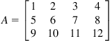
We have three rows and four columns. In our memory space, each element is stored as

In the MATLAB command window, we write this as
A=[1 2 3 4; 5 6 7 8; 9 10 11 12]
In c-mex, this matrix is passed as one of the arguments in prhs. Assuming this is a first input element, we get this matrix as a single-precision piece of data in the gateway routine, then we obtain a pointer as
float* ptr=(float*)mxGetData(prhs[0]);
In C/C++, using a zero-based index,1 we access each element using the pointer arithmetic. To get the value, 10, we write
ptr[5]
or
*(ptr+5)
In general, to access a 2D matrix element at m-th row and n-th column of M×N matrix, we calculate the pointer offset and access it as
ptr[ (n * M)+m ]
or
*(ptr+(n * M)+m)
For 3D arrays, M×N×P, we access the m-th row, n-th column, p-th depth as
ptr[ ( p * N+n) * M+m ]
or
As you can see, when accessing data sequentially in memory, the row index varies more quickly than the column index varies.
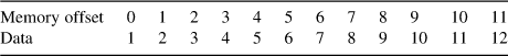
The following example shows memory locations of 2D array in c-mex. A simple array is passed to our c-mex function, and we just print out each array element and its corresponding memory address in our MATLAB command window for both single-precision and byte data types.
For single-precision data types,
// column_major_order_single.cpp
#include "mex.h"
void mexFunction(int nlhs, mxArray *plhs[], int nrhs, const mxArray *prhs[])
{
if (!mxIsSingle(prhs[0]))
mexErrMsgTxt("input vector data type must be single");
int rows=(int)mxGetM(prhs[0]);
int cols=(int)mxGetN(prhs[0]);
int totalElements=rows * cols;
float* A=(float*)mxGetData(prhs[0]);
for (int i=0; i<totalElements; ++i)
     mexPrintf("%f at %p
", A[i], A+i);
}
>> mex column_major_order_single.cpp
>> column_major_order_single(single([1 2 3 4; 5 6 7 8; 9 10 11 12]))
1.000000 at 0x128406240
5.000000 at 0x128406244
9.000000 at 0x128406248
2.000000 at 0x12840624c
6.000000 at 0x128406250
10.000000 at 0x128406254
3.000000 at 0x128406258
7.000000 at 0x12840625c
11.000000 at 0x128406260
4.000000 at 0x128406264
8.000000 at 0x128406268
12.000000 at 0x12840626c
(You can test this with our example column_major_single.m.)
Note that each data element occupies 4 bytes, which is a typical byte size for single-precision data.
The next example demonstrates the single-byte data type, 8-bit unsigned integer:
// column_major_order_unit8.cpp
#include "mex.h"
void mexFunction(int nlhs, mxArray *plhs[], int nrhs, const mxArray *prhs[])
{
if (!mxIsUint8(prhs[0]))
mexErrMsgTxt("input vector data type must be single");
int rows=(int)mxGetM(prhs[0]);
int cols=(int)mxGetN(prhs[0]);
int totalElements=rows * cols;
unsigned char* A=(unsigned char*)mxGetData(prhs[0]);
for (int i=0; i<totalElements; ++i)
     mexPrintf("%f at %p
", A[i], A+i);
}
>> mex column_major_order_uint8.cpp
>> column_major_order_uint8(uint8([1 2 3 4;5 6 7 8; 9 10 11 12]))
1 at 0x128408960
5 at 0x128408961
9 at 0x128408962
2 at 0x128408963
6 at 0x128408964
10 at 0x128408965
3 at 0x128408966
7 at 0x128408967
11 at 0x128408968
4 at 0x128408969
8 at 0x12840896a
12 at 0x12840896b
(You can test this with our example column_major_uint8.m.)
As you may notice, in the single-precision data type, the memory address jumps 4 bytes, whereas 8-bit unsigned integer increments jump by 1 byte.
4.2.2 Row-Major Order
Row-major order is exactly the opposite of column-major order. Consider the same example matrix:
a=[1 2 3 4; 5 6 7 8; 9 10 11 12]
The value, 10, can be accessed as
ptr[9]
or
*(ptr+9)
For 2D arrays, the element at m-th row and n-th column of an M×N matrix is accessed as
ptr[ ( m * N )+n ]
or
*(ptr+(m * N)+n)
and for a 3D array, the element at m-th row, n-th column, and p-th depth of an M×N×P array is accessed as
ptr[ ( p * M+m ) * N+n ]
or
*(ptr+(p * M+m) * N+n)
Here, the column index varies more quickly than the row index varies.
When we mingle C/C++ and MATLAB, we need to be very mindful about how input data are stored and indexed. For instance, many C/C++ image libraries store images in row-major order while data passed from MATLAB is in column-major order. In CUDA, threads are accessed based on row-major order. Another important thing we must keep in mind is the indexing scheme. C/C++ uses a zero-based index, while MATLAB accesses the array element using a one-based index.
4.2.3 Memory Layout for Complex Numbers in c-mex
Often, we face complex numbers in many aspects. Especially in image or signal processing, our data are either complex or real numbers or both. Through algorithms, they change from real to complex numbers or from complex to real numbers. Therefore, we want to make sure that we understand how MATLAB packs our complex number in memory space when we receive it from or pass it back to MATLAB in our c-mex function.
When storing a complex number in memory, we can put the real part first then the imaginary part or vice versa. Typically, a complex number is stored with real part first. For instance, a complex number, C=3+7i, is stored as
| Memory offset | 0 | 1 |
| Data | 3 | 7 |
Let us quickly experiment to see how MATLAB stores our complex number:
// TestComplex1.cpp
#include "mex.h"
void mexFunction(int nlhs, mxArray *plhs[], int nrhs, const mxArray *prhs[])
{
if (!mxIsComplex(prhs[0]))
mexErrMsgTxt("input data must be complex");
if (!mxIsSingle(prhs[0]))
mexErrMsgTxt("input data must be single");
float* pReal = (float*)mxGetPr(prhs[0]);
float* pImag = (float*)mxGetPi(prhs[0]);
  mexPrintf("%p: %f
", pReal, *pReal);
  mexPrintf("%p: %f
", pImag, *pImag);
}
Compile this test c-mex code and run with a sample number.
>> mex TestComplex1.cpp
>> TestComplex1(single(4+5i))
000000006F2FBB80: 4.000000
000000006F2FC940: 5.000000
(You can test this with our example TestComplex_first.m.)
The real part of our sample number is stored at 0x6F2FBB80, while the imaginary part of the number is at 0x6F2FC940. As you can see, they are not next to each other. As a matter of fact, MATLAB stores complex numbers in two separate arrays. For this reason, it provides two functions to access these arrays. Using mxGetPr(…) gives us the pointer to the array for the real number, while mxGetPi(…) is for the imaginary number. We can modify a little bit our test program and see what happens when our data are an array of complex numbers:
#include "mex.h"
void mexFunction(int nlhs, mxArray *plhs[], int nrhs, const mxArray *prhs[])
{
if (!mxIsComplex(prhs[0]))
mexErrMsgTxt("input data must be complex");
if (!mxIsSingle(prhs[0]))
mexErrMsgTxt("input data must be single");
float* pReal=(float*)mxGetPr(prhs[0]);
float* pImag=(float*)mxGetPi(prhs[0]);
int n=(int)mxGetN(prhs[0]);
int numElems=(m >= n) ? m : n;
for (int i=0; i<numElems; ++i, ++pReal, ++pImag)
{
mexPrintf("Real=%f @%p ", *pReal, pReal+i);
    mexPrintf("Imag=%f @%p
", *pImag, pImag+i);
}
}
When compiled and run with a sample complex array, we get data as follows:
>> mex TestComplex.cpp
>> TestComplex(single([1+10i, 2+20i, 3+30i, 4+40i]))
Real=1.000000 @000000006F60A4A0 Imag=10.000000 @000000006F60A420
Real=2.000000 @000000006F60A4A8 Imag=20.000000 @000000006F60A428
Real=3.000000 @000000006F60A4B0 Imag=30.000000 @000000006F60A430
Real=4.000000 @000000006F60A4B8 Imag=40.000000 @000000006F60A438
(You can test this with our example TestComplex_second.m.)
We see clearly two different arrays for each part of complex number (Figure 4.1).
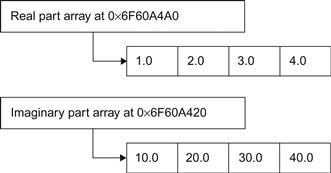
If our input data are two-dimensional complex numbers, we receive two 2D arrays for each part: a 2D array of the real part and a 2D array of the imaginary part. And remember that they are column-major ordered.
4.3 Logical Programming Model
When we write a CUDA program (.cu file), we use special syntax, <<<⋅⋅⋅>>>, on functions that need to be run on the GPU. In Chapter 2, we had the example AddVectors.cu.

The section of code that runs on GPU is called a kernel. When we define a kernel, we have to explicitly specify the total number of threads in which that kernel will be run. Basically, the same kernel will be run in parallel in multiple threads. We tell the GPU how many threads we would like to run in parallel. Depending on how many parallel jobs we need, we figure out how many threads are needed. Those threads are then logically grouped into a block. A group of blocks composes a grid. This logical grouping information is passed to the GPU inside the <<<⋅⋅⋅>>>:
Kernel_Function <<<gridSize, blockSize >>> (parameter1, parameter2,….)
A grid size is specified by its number of blocks. A block size is specified by its number of threads. For instance, if the grid size is 10, then there are 10 blocks in a grid. If the block size is 5, then there are 5 threads in a block. Therefore, if we say that a grid size is 10 and a block size is 5, then it means there are 50 threads in total.
Let us compare a CPU code and a GPU code. In the CPU code, the additions in operation_at_cpu(..) occur by iteration within a loop. The iteration conditions are explicitly set by the serial setting (i=0; i<N; i++) in a for-loop. The corresponding part in GPU code performs the additions by a number of threads in parallel. The parallelization conditions are set by the combination of CUDA’s built-in device variables (blockDim, blockIdx and threadIdx). The device variables such as blockDim, blockIdx, and threadIdx are limited by the gridSize and blockSize inside the <<<…>>> when we call the kernel. The actual parallel running is automatically activated by the GPU device when it is called. We deal with the blockDim, blockIdx and threadIdx in Section 4.5:

In CUDA, it is our responsibility to tell GPU how many threads we need to run in parallel and how they are logically grouped into blocks and grids.
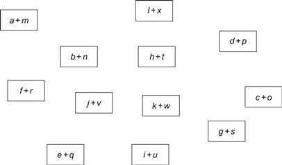
Suppose we have a simple matrix addition of size 3×4:

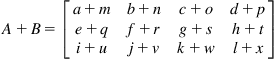
We can easily identify 12 independent additions that can be run in parallel. We can tell GPU in various ways how to group these threads in terms of grids and blocks (Figure 4.2).
4.3.1 Logical Grouping 1
These 12 independent additions can be grouped individually so that there are 12 blocks in a grid and each block with one thread only (Figure 4.3).

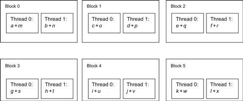
4.3.2 Logical Grouping 2
Another way of grouping these threads would be 6 blocks in a grid and two threads per block (Figure 4.4).
4.3.3 Logical Grouping 3
CUDA also provides ways to specify the groupings in two or three dimensions. We could group these threads into 2×2 blocks per grid and 2×3 threads per block. This creates 24 threads in total, which is twice as many threads as we need (Figure 4.5).
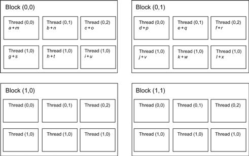
Notice that some blocks have empty threads and do not need to do any calculation. We tell GPU that there are 24 threads but only 12 threads are the real ones. In our kernel, we skip these empty threads by checking its thread index.
Naturally, you ask how we should group them. To answer this question, let us briefly take a look at some details of GPU hardware.
4.4 Tidbits of GPU
Based on the time performance profile we measured, the CUDA counterpart of the 2D convolution algorithm in Chapter 2 is very disappointing. Let us sit back and think a bit about what went wrong with our naïve approach to CUDA programming. As you might already know, the key to success in CUDA programming is very closely related to understanding GPU architecture. Let us briefly review how GPU is designed, so that we are better equipped with our tools.
4.4.1 Data Parallelism
Unlike CPU, GPU has been designed with the goal in mind for high throughput, so that it can process, for example, a same triangular mesh operation on millions of pixels for a given frame in graphics. As a matter of fact, GPU runs thousands of threads concurrently. This is a whole lot of threads compared to CPU, and it opens new ways for parallel processing number crunching activities. For this reason, when we can achieve data parallelism, GPU fits in naturally for its capability to run thousands of threads. Achieving data parallelism should be the foremost step. In our example of image convolution, each pixel could be independently processed in parallel with other pixels. If we have 10×10 size of image, we could assign each pixel to each thread and have all the 100 threads processed at the same time.
On hardware side, GPU uses a single instruction, multiple data (SIMD) model, where one single instruction can run on multiple different data. Compared to CPU, GPU has many more cores and registers to handle thousands of lightweight threads. GPU also schedules all those threads at the hardware level. Context switching requires almost zero overhead, whereas context switching in CPU is costly.
4.4.2 Streaming Processor
A fundamental unit of GPU is a streaming processor (SP). This provides the capability to fetch a single instruction from memory and carry it out on different data sets in parallel. Each GPU contains tens to hundreds of SPs in a single piece of hardware.
4.4.3 Steaming Multiprocessor
Each SP is then grouped as a streaming multiprocessor (SM). The SM provides thousands of registers, a thread scheduler, and shared memory for the group of SPs. Equipped with those components in its silicon backyard and a number of SPs, an SM manages thread scheduling, context switching, and data fetching and caching for the blocks of threads assigned to it.
4.4.4 Warp
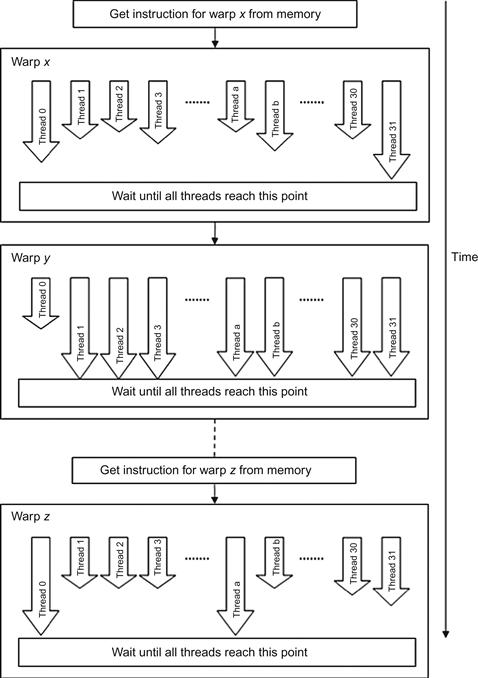
The SM especially schedules threads in groups of 32 parallel threads called, warp. All threads in the same warp share a single instruction fetch from memory. All threads in each warp march at the same pace. A SM processes the next warp only when all the threads in the current warp finish their jobs. For instance, if one thread takes 10 seconds to finish its job while the rest of the threads take 1 second, the SM hase to wait 9 more seconds until it is ready to move to the next warp.
Overall, GPU receives a number of grids. Blocks from grids are then assigned to SMs. The SM assigns threads to SPs and manages them in a unit called a warp, as illustrated in Figures 4.6 and 4.7. Threads are processed in a group called a warp. The actual physical number of concurrent threads is limited by the number of SPs. The SM is responsible for scheduling the threads in warps.

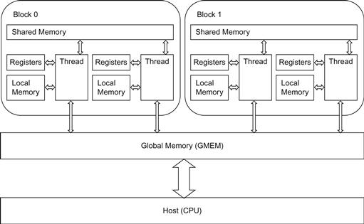
4.4.5 Memory
Three major types of memory spaces are available. The first type of memory is global memory. This is the memory space accessible by both GPU and CPU. Usually, on CPU side, we first allocate on GPU using this global memory and copy our data from CPU side of memory to here. Also, this space is accessible to all grids and subsequently to all threads. Specifically, we use CUDA runtime API calls like cudaMalloc and cudaMemcpy to allocate and to copy data from GPU to CPU and vice versa.
The second type of memory is shared memory. Not all threads have access to this. Only the threads in the same block can access it. However, access time is much faster than that of global memory. We can allocate this type of memory using a keyword, __shared__. If values need to and can be shared within a block of threads, putting them for these threads in shared memory greatly reduces the memory access time overhead.
The third type is a memory space available only to each thread. It is the per-thread local memory using registers. Unlike CPU, GPU has thousands of registers per SM. They are dedicated for each thread and provide almost zero overhead thread context switching. Declaring data as a local variable in the kernel lets us use registers. However, the capacity of local memory in a kernel is very limited, and for this reason, we must ensure that we do not abuse it with excessive usage. When registers cannot accommodate the requested amount, it will place them at local memory that is local to the thread but does not give us as fast access time as registers.
Figure 4.8 shows an overview of memory in GPU.
4.5 Analyzing Our First Naïve Approach
Our first CUDA implementation of two-dimensional convolution turned out to be much slower than the native MATLAB function conv2. Equipped with knowledge of the inside of GPU, we are ready to tackle the problem. In our first approach, we mindlessly assigned a thread in each block and each block in one grid. This gave us the total number of threads we needed to run. We declared the kernel as
dim gridSize(numRows, numCols)
conv2MexCuda<<<gridSize, 1>>>
With this declaration, there are numRows×numCols blocks and each block contains one thread. Thus, we have the total of numRows×numCols threads. Remember, in MATLAB, data are passed to us in column-major order. So we assigned numRows first then numCols. In Figure 4.9, as we move horizontally, the first index of the block maps to the number of rows, while the second index maps to the number of columns. Each thread in a block handles each pixel in our input image.

Blocks of each grid are scheduled to SMs, and each SM schedules threads in the warp. When a SM processes threads, only one thread will run in each warp. But, a SM can handle 32 threads in a warp. Since there is only one thread in a warp, most of SPs in SMs sit idle. We heavily under-utilize GPU resources.
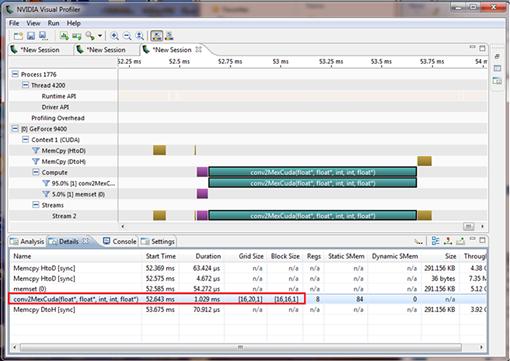
Let us run NVIDIA Visual Profiler once again to see how it performs when we assign each thread to each block (Figure 4.10).
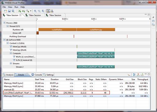
As we can see in the Details tab, the kernel itself takes about 33 msec when our grid size is the same as the image size. Each thread handles each pixel. With the naïve approach, we even make our CUDA-based convolution worse than the MATLAB native function. Therefore, in this case, we gain no advantage from GPU acceleration. In the next section, we try to resize our grids and blocks so that we can utilize rest of the threads in the warp in the SM.
4.5.1 Optimization A: Thread Blocks
In this optimization step, we try to optimize by resizing the grid and block. First, we decide a block size to be 16×16. This gives us a total of 256 threads in a block, and obviously, it is greater than the warp size. Based on this block size and the image size, we determine the grid size. By having more threads in a block, we can utilize rest of the threads in the block, whereas in the naïve approach, we utilize only one thread per block.
Each of our new blocks consists of 256 threads arranged two-dimensionally as Figure 4.11. Each thread in the block processes each pixel in the input image. Figure 4.12 shows the original input image from MATLAB.
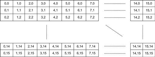

For illustration purpose, let us first transpose the input image, since the input image coming from MATLAB is in column-major order and it is stored in row-major order in C/C++ and CUDA. Then, we put our blocks on top of it to see how the original image is divided into blocks and threads (Figure 4.13).

Given the size of the input image and the block size, we can determine how many blocks fit both horizontally and vertically. Note that the total area covered by the blocks is larger than the input image. This is because all the blocks should be the same size while the image size may not be in multiples of our block size. Therefore, we make the area covered by blocks larger than the image size.
dim3 blockSize(16, 16);
dim3 gridSize((numRows +15) / blockSize.x, (numCols+15) / blockSize.y);
This code snippet shows how we calculate the smallest number that is a multiple of 16 and equal to or greater than the image size. We introduce two variables, blockSize and gridSize, of dim3 type.
Now, the each pixel in the image can be accessed by the thread index and block sizes as we assign each pixel to each thread. When the CUDA kernel is called, we can access information about which thread and where in the block we are processing. Inside the kernel, we use the following global variables from CUDA to find out the exact pixel locations.
Each specific pixel location can be calculated using these variables as shown in Figure 4.14. Note again that the rows of the image are presented horizontally while the columns are presented vertically, because the memory layout of our image in MATLAB is in column-major order.
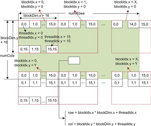
Those threads assigned to pixels outside the image just return without doing any processing. The border area of our convolution operation is also ignored. Inside the kernel, we check if it is outside the boundary or the border as
int row=blockIdx.x * blockDim.x+threadIdx.x;
if (row<1 || row>numRows−1)
return;
int col=blockIdx.y * blockDim.y+threadIdx.y;
if (col<1 || col>numCols−1)
Let us now create a new file and save it as conv2MexOptA.cu.
#include "conv2Mex.h"
__global__ void conv2MexCuda(float* src,
float* dst,
int numRows,
int numCols,
float* mask)
{
int row=blockIdx.x * blockDim.x+threadIdx.x;
if (row<1 || row>numRows−1)
return;
int col=blockIdx.y * blockDim.y+threadIdx.y;
if (col<1 || col>numCols−1)
return;
int dstIndex=col * numRows+row;
dst[dstIndex]=0;
int mskIndex=3 * 3−1;
for (int kc=−1; kc<2; kc++)
{
int srcIndex=(col+kc) * numRows+row;
for (int kr=−1; kr<2; kr++)
{
dst[dstIndex] += mask[mskIndex−−] * src[srcIndex+kr];
}
}
}
void conv2Mex(float* src, float* dst, int numRows, int numCols, float* msk)
{
int totalPixels=numRows * numCols;
float *deviceSrc, *deviceMsk, *deviceDst;
cudaMalloc(&deviceSrc, sizeof(float) * totalPixels);
cudaMalloc(&deviceDst, sizeof(float) * totalPixels);
cudaMalloc(&deviceMsk, sizeof(float) * 3 * 3);
cudaMemcpy(deviceSrc, src, sizeof(float) * totalPixels, cudaMemcpyHostToDevice);
cudaMemcpy(deviceMsk, msk, sizeof(float) * 3 * 3, cudaMemcpyHostToDevice);
cudaMemset(deviceDst, 0, sizeof(float) * totalPixels);
dim3 blockSize(16, 16);
dim3 gridSize((numRows +15) / blockSize.x, (numCols+15) / blockSize.y);
conv2MexCuda<<<gridSize, blockSize>>>(deviceSrc,
numRows,
numCols,
deviceMsk);
cudaMemcpy(dst, deviceDst, sizeof(float) * totalPixels, cudaMemcpyDeviceToHost);
cudaFree(deviceSrc);
cudaFree(deviceDst);
cudaFree(deviceMsk);
}
In this example code, we create a new kernel and call it as folows:
conv2MexCuda<<<gridSize, blockSize>>>(deviceSrc,
deviceDst,
numRows,
numCols,
deviceMsk);
We passed new block and thread sizes to our kernel. Instead of processing each pixel at each block, we regrouped into 16×16 thread blocks. But, each thread performed 3×3 mask multiplication and addition as before.
Then, we profiled this new approach with the NVIDIA Visual Profiler. We now see huge improvement over our first naïve approach. We achieved a time profile more than 30 times faster (Figure 4.15).

4.5.2 Optimization B
In this optimization step, we leave everything intact but introduce a shared memory in the CUDA kernel. When calculating convolution at each pixel, we use the same nine mask values over and over again. We query these values from the global memory every time we apply the mask. Getting these values from the GPU global memory is costly compared to getting them from a shared memory or registers. So, this motivates us to put the mask values in the shared memory and use them to minimize the global memory access overhead.
Inside our kernel, we declare
__shared__ float sharedMask[9];
This creates a shared memory in GPU, and it is shared by all the threads in a block. So, all 256 threads in a block use this shared memory. We then use the first nine threads to fill the shared memory with the mask values. After we prepare our shared memory with the convolution mask values, we process the actual calculation. To ensure that no other thread continues calculation before we fill in the shared memory, we call
__syncthreads();
Now, we create and save a new file, convMexOptB.cu, as follows:
#include "conv2Mex.h"
__global__ void conv2MexCuda(float* src,
float* dst,
int numRows,
int numCols,
float* mask)
{
int row=blockIdx.x * blockDim.x+threadIdx.x;
int col=blockIdx.y * blockDim.y+threadIdx.y;
if (row<1 || row>numRows−1 || col<1 || col>numCols−1)
return;
__shared__ float sharedMask[9];
if (threadIdx.x<9)
{
sharedMask[threadIdx.x]=mask[threadIdx.x];
__syncthreads();
int dstIndex=col * numRows+row;
dst[dstIndex]=0;
int mskIndex=8;
for (int kc=−1; kc<2; kc++)
{
int srcIndex=(col+kc) * numRows+row;
for (int kr=−1; kr<2; kr++)
{
dst[dstIndex] += sharedMask[mskIndex−−] * src[srcIndex+kr];
}
}
}
void conv2Mex(float* src, float* dst, int numRows, int numCols, float* msk)
{
int totalPixels=numRows * numCols;
float *deviceSrc, *deviceMsk, *deviceDst;
cudaMalloc(&deviceSrc, sizeof(float) * totalPixels);
cudaMalloc(&deviceDst, sizeof(float) * totalPixels);
cudaMalloc(&deviceMsk, sizeof(float) * 3 * 3);
cudaMemcpy(deviceSrc, src, sizeof(float) * totalPixels, cudaMemcpyHostToDevice);
cudaMemcpy(deviceMsk, msk, sizeof(float) * 3 * 3, cudaMemcpyHostToDevice);
cudaMemset(deviceDst, 0, sizeof(float) * totalPixels);
const int size=16;
dim3 blockSize(size, size);
dim3 gridSize((numRows+size−1) / blockSize.x,
(numCols+size−1) / blockSize.y);
conv2MexCuda<<<gridSize, blockSize>>>(deviceSrc,
deviceDst,
numRows,
numCols,
deviceMsk);
cudaMemcpy(dst, deviceDst, sizeof(float) * totalPixels, cudaMemcpyDeviceToHost);
cudaFree(deviceSrc);
cudaFree(deviceDst);
cudaFree(deviceMsk);
We introduced the shared memory. Since values in the kernel are the same for all pixels, we put the kernel values in the shared memory, so that 16×16 threads can share the same kernel values from the L1 cache instead of fetching the values from the global memory.
We compile the preceding and run the code using the NVIDIA Visual Profiler. We now get the result shown in Figure 4.16. We achieved a little improvement over our first optimization step.
4.5.3 Conclusion
We see now that the overall performance did improve very much from our very first naïve method. But, we are still behind the native MATLAB function conv2 when considering the end-to-end function call. What makes us slower overall? Remember, we do cudaMemcpy whenever we call our function. We copy values to and from host memory to GPU device memory every time we invoke our method. This adds a lot of overhead, while the actual convolution inside GPU is much faster. So, we may want to do as much computation as possible inside GPU, minimizing data transfer between the host and the device.
1Note that every matrix index in MATLAB starts with 1, while a C/C++ array index starts with 0.