Accelerating MATLAB without GPU
This chapter deals with basic accelerating methods for MATLAB codes in an intrinsic way, which means simple code optimization without using GPU or C-MEX. This chapter covers vectorization for parallel processing, preallocation for efficient memory management, tips to increase your MATLAB codes, and step-by-step examples that show the code improvements.
Keywords
Vectorization; elementwise operation; vector/matrix operation; memory preallocation; sparse matrix form
1.1 Chapter Objectives
In this chapter, we deal with the basic accelerating methods for MATLAB codes in an intrinsic way – a simple code optimization without using GPU or C-MEX. You will learn about the following:
1.2 Vectorization
Since MATLAB has the vector/matrix representation of its data, “vectorization” can help to make your MATLAB codes run faster. The key for vectorization is to minimize the usage of a for-loop.
Consider the following two m files, which are functionally the same:
The left nonVec1.m has a for-loop to calculate the sum, while the right Vec1.m has no for-loop in the code.
>> nonVec1
Elapsed time is 0.944395 seconds.
y =
−1.3042e+48
>> Vec1
Elapsed time is 0.330786 seconds.
y =
−1.3042e+48
The results are same but the elapsed time for Vec1.m is almost three times less than that for nonVec1.m. For better vectorization, utilize the elementwise operation and vector/matrix operation.
1.2.1 Elementwise Operation
The * symbol is defined as matrix multiplication when it is used on two matrices. But the .* symbol specifies an elementwise multiplication. For example, if x = [1 2 3] and v = [4 5 6],
>> k = x .* v
k =
4 10 18
Many other operations can be performed elementwise:
>> k = x .^2
k =
1 4 9
>> k = x ./ v
k =
0.2500 0.4000 0.5000
Many functions also support this elementwise operation:
>> k = sqrt(x)
k =
1.0000 1.4142 1.7321
>> k = sin(x)
k =
0.8415 0.9093 0.1411
>> k = log(x)
k =
0 0.6931 1.0986
>> k = abs(x)
k =
1 2 3
Even the relational operators can be used elementwise:
>> R = rand(2,3)
R =
0.8147 0.1270 0.6324
0.9058 0.9134 0.0975
>> (R > 0.2) & (R < 0.8)
ans =
0 0 1
0 0 0
>> x = 5
x =
5
>> x >= [1 2 3; 4 5 6; 7 8 9]
ans =
1 1 1
1 1 0
0 0 0
We can do even more complicated elementwise operations together:
>> A = 1:10;
>> B = 2:11;
>> C = 0.1:0.1:1;
>> D = 5:14;
>> M = B ./ (A .* D .* sin(C));
1.2.2 Vector/Matrix Operation
Since MATLAB is based on a linear algebra software package, employing vector/matrix operation in linear algebra can effectively replace the for-loop, and result in speeding up. Most common vector/matrix operations are matrix multiplication for combining multiplication and addition for each element.
If we consider two column vectors, a and b, the resulting dot product is the 1×1 matrix, as follows:


If two vectors, a and b, are row vectors, the ![]() should be
should be ![]() to get the 1×1 matrix, resulting from the combination of multiplication and addition, as follows.
to get the 1×1 matrix, resulting from the combination of multiplication and addition, as follows.
In many cases, it is useful to consider matrix multiplication in terms of vector operations. For example, we can interpret the matrix-vector multiplication ![]() as the dot products of x with the rows of A:
as the dot products of x with the rows of A:
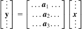
![]()
1.2.3 Useful Tricks
In many applications, we need to set upper and lower bounds on each element. For that purpose, we often use if and elseif statements, which easily break vectorization. Instead of if and elseif statements for bounding elements, we may use min and max built-in functions:
>> ifExample
Elapsed time is 0.878781 seconds.
y =
5.8759e+47
>> nonifExample
Elapsed time is 0.309516 seconds.
y =
5.8759e+47
Similarly, if you need to find and replace some values in elements, you can also avoid if and elseif statements by using the find function to keep vectorization.
Vector A is compared with scalar 0.5 in elementwise fashion and returns a vector of the same size as A with ones for matched positions. The find function gives the indices of matched positions then replaces the original value.
1.3 Preallocation
Resizing an array is expensive, since it involves memory deallocation or allocation and value copies each time we resize. So, by preallocating the matrices of interest, we can get a pretty significant speedup.
>> preAlloc
Elapsed time is 0.000032 seconds.
Elapsed time is 0.000014 seconds.
In the preceding example, the array x is resized by reallocating the memory and setting the values more than once, while the array y is initialized with zeros(4,1). If you do not know the size of matrix before the operation, it would be a good idea to first allocate an array that will be big enough to hold your data, and use it without memory reallocation.
1.4 For-Loop
In many cases, it is inevitable that we need to use a for-loop. As a legacy of Fortran, MATLAB stores matrix in a column-major order, where elements of the first column are stored together in order, followed by the elements of the second column, and so forth. Since memory is a linear object and the system caches values with their linear neighbors, it would be better to make the nested loop for your matrix, column by column.
>> row_first
Elapsed time is 9.972601 seconds.
>> col_first
Elapsed time is 7.140390 seconds.
The preceding col_first.m is almost 30% faster than row_first.m by the simple switch of the i and j in the nested for-loop. When we use huge higher dimensional matrices, we can expect greater speed gain from the column-major operation.
1.5 Consider a Sparse Matrix Form
For handling sparse matrices (large matrices of which the majority of the elements are zeros), it is a good idea to consider the use of the “sparse matrix form” in MATLAB. For very large matrices, the sparse matrix form requires less memory because it stores only nonzero elements, and it is faster because it eliminates operations on zero elements.
The simple way to create a matrix in sparse form is as follows:
>> i = [5 3 6] % used for row index
>> j = [1 6 3] % used for column index
>> value = [0.1 2.3 3.1] % used for values to fill in
>> s = sparse (i,j,value) % generate sparse matrix
s =
(5,1) 0.1000
(6,3) 3.1000
(3,6) 2.3000
>> full = full(s) % convert the sparse matrix to full matrix
full =
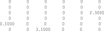
Or simply convert the full matrix to a sparse matrix using the sparse built-in command:
>> SP = sparse(full)
SP =
(5,1) 0.1000
(6,3) 3.1000
(3,6) 2.3000
All of the MATLAB built-in operations can be applied to the sparse matrix form without modification, and operations on the sparse matrix form automatically return results in the sparse matrix form.
The efficiency of the sparse matrix form depends on the sparseness of the matrix, meaning that the more the zero elements the matrix has, the speedier the matrix operation will be. If a matrix has very little or no sparseness, speeding up and memory saving benefits from using the sparse matrix form no longer can be expected.
>> denseSparse
Elapsed time is 5.846979 seconds.
Elapsed time is 41.050271 seconds.
>> RealSparse
Elapsed time is 5.879175 seconds.
Elapsed time is 3.798073 seconds.
In the DenseSparse.m example, we tried to convert the dense matrix (A: 5000×5000) to the sparse matrix (sp_denseA). The operation with sparse matrix form takes much more time than that of dense matrix calculation. In the RealSparse.m example, however, we speed up a lot from the sparse matrix form. The function sprand(5000, 2000, 0.2) generates 5000×2000 elements. The third parameter, 0.2, means that about 20% of the total elements are nonzero elements and other 80% are zero elements within the generated matrix. The sparse matrix with even 20% nonzero elements can achieve much greater speed in matrix operations.
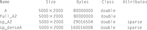
When we look at the memory size required for each matrix, as in the following, the sparse form (sp_A2) from the sparse matrix requires much less memory size (about 29 MB) than the full matrix form (80 MB). However, the sparse form (sp sp_denseA) from the dense matrix requires much more memory (about 160 MB) than its full matrix form (80 MB), because the sparse matrix form requires extra memory for its matrix index information in addition to its values.
>> whos('A', 'sp_denseA','full_A2','sp_A2')
1.6 Miscellaneous Tips
1.6.1 Minimize File Read/Write Within the Loop
Calling functions involving file read/write is very expensive. Therefore, we should try to minimize or avoid its use especially within a loop. The best way for handling file read/write is to read files and store data into variables before the loop, and then use those stored variables inside the loop. After you exit the loop, write the results back to the file.
It seems simple and obvious to avoid file reading/writing within loop, but when we use many functions over multiple files, the file reading/writing parts can inadvertently reside within the deep inner loop. To detect this inadvertent mistake, we recommend the profiler to analyze which parts of a code significantly affect the total processing time. We deal with the use of a profiler in Chapter 3.
1.6.2 Minimize Dynamically Changing the Path and Changing the Variable Class
Similar to the file reading/writing, setting a path is also expensive. So it should be minimized. It is also recommended to set the path outside the loop. Changing the variable/vector/matrix class is also expensive. So it should also be minimized, especially within loops.
1.6.3 Maintain a Balance Between the Code Readability and Optimization
Although we emphasize the code optimization so far, the code maintenance is a very important factor for designing/prototyping algorithm. Therefore, it is not always a good idea to trade off code readability with heavy optimizations. Please try to make a balance between code readability and optimization, from which we can get more benefits by saving costly debugging times while spending more on creative algorithms and living a happier life.
1.7 Examples
When you run myDisplay.m, you see a figure like Figure 1.1. In this example, we are going to search for a black book (template image on the left) out of 12 objects (right). Since both the template and object images are in color, the dimensions of both images are three dimensions (x, y, and color). Although the original size of the object image on the right is 1536×2048×3 and the size of the template image on the left is 463×463×3, each object in the right image is picked already to have the same size as the template image (Figure 1.2) to reduce unnecessary details for the purpose of demonstration. Also those 12 objects are stored in a big matrix v in the compareImageVector.mat with “unrolled” forms. So the 463×463×3 matrix for one object is unrolled to a 1×643107 row vector, and the matrix v has 12 rows for a total of 12 objects (12×643107 matrix).

Figure 1.1 Object detection example using a template image.
In this example, the black book on the left is used as a template image to search the 12 objects on the right. Notice that a black book on the right is rotated slightly and has some shading around its background.
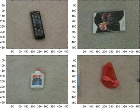
Figure 1.2 Every object is already picked to have the same size as the template image for simplicity.
Our first naïve m code follows:
This m file tries to calculate the normalized cross-correlation to compare each image with the template image.
![]()
Here, T(x, y) is each pixel value for the template image, ![]() is the average pixel value for the template image, and σT is the standard deviation, while I(x, y) is each pixel value for each object image to be compared. So, when we have a higher normalized cross-correlation value, it means that the two images being compared are more similar. In this example, we will try to find the object with the highest normalized cross-correlation value, as it is most similar to the template image.
is the average pixel value for the template image, and σT is the standard deviation, while I(x, y) is each pixel value for each object image to be compared. So, when we have a higher normalized cross-correlation value, it means that the two images being compared are more similar. In this example, we will try to find the object with the highest normalized cross-correlation value, as it is most similar to the template image.
compareVec_LoopNaive.m results out like this:
>> compareVec_LoopNaive
Elapsed time is 65.008446 seconds.
y =
1.0e+05 *
0.2002
1.2613
2.9765
2.6793
2.6650
−0.0070
2.7570
0.7832
0.3291
5.0278
2.8071
−0.5271
From this result, the 10th line of the normalized cross-correlation has the highest value (5.0278 * E05), which is the 10th object in the Figure 1.1. Although the result was good enough to find the right object (Figure 1.3), we may do a few things to improve its speed. Before going to next pages, please try to find the parts that can be improved from the compareVec_LoopNaive.m file by yourself.
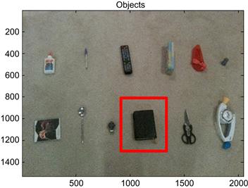
Figure 1.3 Comparing the result with the template image using the normalized cross-correlation.
The 10th object was chosen to have the highest normalized cross-correlation value.
Let us start to look over the code carefully. Do you remember that the preallocation can speed up MATLAB code? Let us do memory allocations for the variable y, normalized_template, and normalized_v by putting the function zero() before they are used (see compareVec_Loop.m below).
The results follow:
>> compareVec_Loop
Elapsed time is 58.102506 seconds.
y =
1.0e+05 *
0.2002
1.2613
2.9765
2.6793
2.6650
−0.0070
2.7570
0.7832
0.3291
5.0278
2.8071
−0.5271
From this simple memory preallocation, we save a lot of running time (from 65 seconds to 58 seconds) easily. Let us tweak the first operation within loop.
Since normalized_v(i,j) = (v(i,j)−mean_v(i)); is the simple subtraction from each row, we can put that line out of loop by vector operation:
mean_matrix = mean_v(:,ones(1,size(v,2)));
normalized_v = v − mean_matrix;
Here, mean_matrix has the same size as the matrix with v by repeating mean_v. From this simple change, we can reduce the running time.
>> compareVec_LoopImprove
Elapsed time is 51.289607 seconds.
y =
1.0e+05 *
0.2002
1.2613
2.9765
2.6793
2.6650
−0.0070
2.7570
0.7832
0.3291
5.0278
2.8071
−0.5271
Let us go further. We use the elementwise operation and vector/matrix operation to avoid using the for-loop. For the elementwise operation, we have
mean_matrix = mean_v(:,ones(1,size(v,2)));
normalized_v = v - mean_matrix;
mean_template = mean(template_vec);
std_template = std(template_vec);
normalized_template = template_vec - mean_template;
These parts can be effectively used to replace the for-loop.
From the vector/matrix operation, we can completely remove the for-loop:
y = normalized_v * normalized_template;
Our final vectorized m-code looks like this:
Its result follows:
>> compareVec
Elapsed time is 0.412896 seconds.
y =
1.0e+05 *
0.2002
1.2613
2.9765
2.6793
2.6650
−0.0070
2.7570
0.7832
0.3291
5.0278
2.8071
−0.5271
This shows that the optimized code is much faster (from 65 seconds to 0.41 seconds without losing accuracy) than the original m code, which had two nested for-loop’s and no preallocation.