
Appendix 1: The Fourier Transform
Chapter Contents
A1.3 The Complex Fourier Series
A1.4 Frequency Analysis of Non-periodic Signals: The Fourier Transform
A1.6 A Fourier Transform Example: The Single Pulse
A1.7 The Discrete Fourier Transform
A1.1 Fourier’s Theorem
Jean Baptiste Joseph Fourier (1768–1830) worked on a mathematical model of heat transfer in solid bodies (amongst many other topics). His thesis On the Propagation of Heat in Solid Bodies was published in 1807 and contained a novel idea for expanding a continuous function as a trigonometric series. Although Fourier developed this as a part of his model for heat transfer, it has a much wider application. Fourier’s theorem is now usually stated as:
Any periodic function can be represented as an infinite sum of harmonic sinusoids multiplied by appropriate coefficients.
Mathematically, this is expressed as:

The periodic function f(t) has a period T0 such that:
![]()
The sum of the sines and cosines on the right-hand side (RHS) of Equation A1.1 is called a Fourier series. The sinusoids are harmonic. This means that all their frequencies are integer multiples of the lowest, or fundamental, frequency ω0.
Equation A1.1 states that, provided we know the correct values for the amplitudes of the sinusoids an and bn, we can add them up and make any periodic signal f(t) we like. Different signals will need different values for an and bn. The act of summing the harmonic sinusoids together to make a signal is called Fourier synthesis. However, we may need an infinite number of harmonics to represent the signal properly. Examples of Fourier synthesis, with their corresponding spectra, were shown in Chapter 1 in Figures 1.50, 1.51 and 1.52 respectively.
These figures also show the effect of not having enough coefficients. We would need an infinite amount to have something that really looked like a square wave.
For the square wave shown in Figure 1.50, its Fourier series coefficients are:

Plotting the magnitude of the coefficients of the Fourier series gives us its frequency spectrum. This is shown in Figure 1.51.
The frequency spectrum tells us how much energy the signal has at any particular harmonic. We can convert Figure 1.51 to a real frequency in Hz simply by multiplying each value of relative frequency, F, by the fundamental frequency, f0.
We can see that the square wave has a lot of energy at the fundamental frequency (F = 1). But the amplitude of the other harmonics decreases quite slowly with frequency. In fact, the harmonic amplitude decreases as 1/F. This slow decay rate is closely associated with the way the square wave looks and how it sounds. A spectrum that falls off as 1/F is always associated with a signal with a discontinuity, and, if its periodic, it will sound “buzzy.”
Odd and Even Functions
There’s something else that’s interesting about the Fourier series of the square wave. Half of its coefficients are zero: all the values of an = 0. This is because the square wave is an odd function. An odd function is one in which f(-t) = −f(t); at any given negative value of t the function is the negative of what it is at the corresponding positive value of t. Look at the square wave again and you’ll see that this is true. Any cosine terms in the Fourier series would ruin this property because the cosine is not an odd function. On the other hand, an even function of time, satisfying f(t) = f(−t), can have only cosine terms in its Fourier series.
However, there are many functions that are neither odd nor even. They will have both a sine and a cosine part to their Fourier series. So in order to plot the magnitude frequency spectrum in this case we must combine the two coefficients together as follows:
![]()
A1.2 Fourier Analysis
The Fourier coefficients discussed earlier are not found by trial and error. Fourier also developed equations for extracting them. For any periodic function, f(t) the harmonic coefficients a0, an and bn can be found from:

A1.3 The Complex Fourier Series
Like many things in acoustics, dealing with the Fourier series in trigonometric form is messy and inconvenient. For example calculating the Fourier series coefficients using the equations in A1.5 requires that we do three integrals! However, by using a complex number theory we can combine the sine and cosine together to form a complex exponential.
![]()
Where θ is in radians.
This allows us to express the Fourier series as a complex exponential as follows:
![]()
Where the now, in general complex coefficients Cn are calculated by:
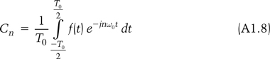
Although in general the coefficients Cn are complex. If the waveform has odd symmetry then resulting coefficients Cn will be purely imaginary (the sine bit), whereas for even symmetry they will be purely real (the cosine bit).
Equations A1.7 and A1.8 can be used instead of Equations A1.1 and A1.5. They also have a further advantage in that when we do a Fourier analysis using Equation A1.4 on a periodic signal, which is neither odd nor even, we end up with two sets of coefficients: the an’s and the bn’s. But when we listen to a periodic sound we only hear one frequency spectrum. Therefore to work out this spectrum we have to combine the an’s and the bn’s to get the total contribution at each frequency, as shown in Equation A1.4.
However, the complex exponential form of the Fourier series automatically gives us a single complex value for the coefficients and by finding their absolute values, or modulus, we get the magnitude of the spectrum, which is usually more perceptually relevant to the listener’s appreciation of timbre. On the other hand the phase of the signal f(t) at each harmonic frequency is given by the argument of each of the complex coefficients Cn.
A1.4 Frequency Analysis of Non-Periodic Signals: The Fourier Transform
The Fourier series is useful for analyzing periodic signals. However, many signals are non-periodic – that is, only occur once. This requires a different approach.
We can consider a single instance of a waveform as being like a periodic signal except that the period is infinity.
If we do this then it possible to state

Where F (ω) is called the Fourier transform of the function f(t). Note that:
- F (ω) replaces the discrete Fourier series coefficients Cn with a continuous function of angular frequency ω.
- The limits of the integral are now theoretically infinite; however, in practice the integral only has to be calculated over the time range where the signal f(t) is non-zero.
- As a matter of convention, time domain signals are represented using lower case letters whereas the frequency domain signals use capitals.
Equation (A1.9) transforms the time domain representation of the signal f(t) into the frequency domain representation of the signal F (ω).
There is a complementary transform that reverses the process and converts the function from the frequency domain back into the time domain, which is:
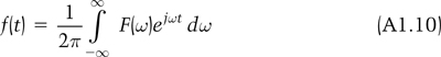
Equations A1.9 and A1.10 are known as the Fourier transform pair and can be used on any type of signal, whether periodic or non-periodic. Together they form a powerful basis for analyzing and processing signals, in particular because it is easier to consider filtering in the frequency domain rather than the time domain.
One way of thinking about this is to remember that the complex exponential representation of a sine wave, ejwt, is a spiral as a function of time, as shown in Figure A1.1, and integration is merely adding up all the numbers within the integration range. Equation A1.5a shows that to get the dc content, all one has to do is add up all the signal values. So what e−jwt is doing, as a spiral in the other direction, is to untwist the waveform at the frequency specified. This converts it to dc where it can be simply extracted by adding up all the dc values in the integration range. The inverse transform re-twists the coefficient to the original frequency, amplitude and phase, and then all the re-twisted sine waves are added up to form the waveform.

Figure A1.1 The complex exponential ejwt, as a spiral as a function of time.
A1.5 The Convolution Theorem
A powerful theorem behind the Fourier transform is the convolution theorem. Convolution is what filters do when they filter signals. However, we normally think about the action of the filter as multiplication of the spectrum of the signal by the filtering function. For example a low-pass filter gets rid of the high frequencies and passes low frequencies. This is expressed using the Fourier transform as the convolution theorem that states:
Convolution in the time domain is equal to multiplication in the transformed (frequency) domain. The converse is also true.
A1.6 A Fourier Transform Example: The Single Pulse
Figure A1.2 shows a single rectangular pulse of length τ seconds and amplitude of 1/τ, which is defined mathematically as follows:

Figure A1.2 A single rectangular pulse of length τ, and amplitude of 1/τ.

Note that irrespective of the value of τ the area of the pulse is constant and equal to one.
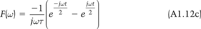
To find the Fourier transform of this we need to use equation A1.11 as f(t) in Equation A1.9. Fortunately, as this function is zero over most of the range and the integral of zero is zero, this results in a solvable definite integral with limits ± (τ/2) that is shown below in Equation A1.12a.


which, after evaluating the limits becomes:
If you remember that:
![]()
and recognize that equation A1.12c can be rearranged to be:
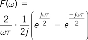
then you can cut straight to Equation A1.12e, instead of taking the “scenic route!”
Expanding out the complex exponentials into cosωτ + jsinωτ gives:

which simplifies to:
![]()
This can be expressed as:

The function sin(x)/x appears so often that it has its own name: sinc(x). So we can say the Fourier transform of the rectangular pulse as described in Equation A1.11, is:
![]()
Note that in this case F(ω) turns out to be real; that is, it has no imaginary part. This is a consequence of our defining f(t) as an even function.
F(ω) is plotted in Figure A1.3 for several values of τ. (Note that as τ gets smaller the frequency extent of the spectrum gets much wider.) It is generally true that a waveform that changes rapidly over a narrow time extent results in a very wide Fourier transform. The converse is also true. In fact if we reduce τ to zero, giving a pulse of infinite amplitude but still with an area equal to one, the spectrum becomes uniform for all frequencies. This infinitely small pulse is called a Dirac delta function and has a uniform, also known as a hite, spectrum. The only other waveform to have a white spectrum is random noise.
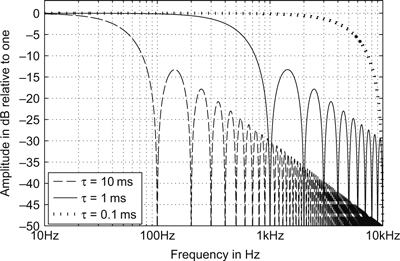
Figure A1.3 The spectrum of a single rectangular pulse of length τ.
A1.7 The Discrete Fourier Transform
With digital audio signals we can calculate something called the discrete Fourier transform, which is given by:
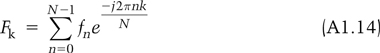
This is a mixture of the continuous Fourier transform defined in Equation A1.9 and the Fourier series in regard to the following:
- The continuous function of time f(t) is replaced by the discrete time sequence xn.
- Continuous time t is replaced by a time index (or sample number) n that takes values 0, 1, 2, … N – 1.
- The length of the signal (or of the chunk being transformed) is N samples and not infinite.
- The integral is replaced by a summation.
- The continuous function of frequency Χ(ω) is replaced by the frequency sequence Xk.
- Continuous frequency f is replaced by frequency index k, which takes values 0, 1, 2, …N – 1. This means that the transform values only exist at a finite number of discrete frequencies. This is a bit like the harmonics in a Fourier series except that there are a finite number of them.
- N discrete input time samples are transformed into N discrete frequency samples whose spacing is proportional to the sampling frequency divided by the number of samples.
There is a corresponding inverse discrete Fourier transform that takes a frequency spectrum and turns it back into a time signal:

The Fourier transform is a powerful tool for the analysis and processing of acoustic signals.