
Acoustic Model for Musical Instruments
Chapter Contents
4.1 A “Black Box” Model of Musical Instruments
4.2.1 Sound source from a plucked string
4.2.2 Sound source from a struck string
4.2.3 Sound source from a bowed string
4.2.4 Sound modifiers in stringed instruments
4.3.1 Sound source in organ flue pipes
4.3.2 Sound modifiers in organ flue pipes
4.3.3 Woodwind flue instruments
4.3.4 Sound source in organ reed pipes
4.3.5 Sound modifiers in organ reed pipes
4.3.6 Woodwind reed instruments
4.4.1 Sound source in percussion instruments
4.4.2 Sound modifiers in percussion instruments
4.5 The Speaking and Singing Voice
4.5.2 Sound modifiers in singing
4.5.3 Tuning in a capella (unaccompanied) singing
4.1 A “Black Box” Model of Musical Instruments
In this chapter a simple model is developed which allows the acoustics of all musical instruments to be discussed and, it is hoped, readily understood. The model is used to explain the acoustics of stringed, wind and percussion instruments as well as the singing voice. A selection of anechoic (no reverberation) recordings of a variety of acoustic instruments and the singing voice is provided on tracks 8–61 on the accompanying CD. Any acoustic instrument has two main components:
- a sound source, and
- sound modifiers.
For the purposes of our simple model, the sound source is known as the “input” and the sound modifiers are known as the “system.” The result of the input passing through the system is known as the “output.” Figure 4.1 shows the complete input/system/output model.
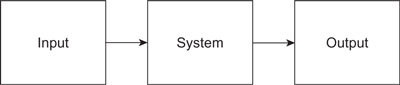
Figure 4.1 An input/system/output model for describing the acoustics of musical instruments.
This model provides a framework within which the acoustics of musical instruments can be usefully discussed, reviewed and understood. Notice that the “output” relates to the actual output from the instrument, which is not that which the listener hears since it is modified by the acoustics of the environment in which the instrument is being played. The input/system/output model can be extended to include the acoustic effects of the environment as follows.
If we are modeling the effect of an instrument being played in a room, then the output we require is the sound heard by the listener and not the output from the instrument itself. The environment itself acts as a sound modifier and therefore it too acts as a “system” in terms of the input/system/output model. The input to the model of the environment is the output from the instrument being played. Thus the complete practical input/system/output model for an instrument being played in a room is shown in Figure 4.2. Here, the output from the instrument is equal to the input to the room.

Figure 4.2 The input/system/output model applied to an instrument being played in a room.
In order to make use of the model in practice, acoustic details are required for the “input” and “system” boxes to enable the output(s) to be determined. The effects of the room are described in Chapter 6. In this chapter, the “input” and “system” characteristics for stringed, wind and percussion instruments as well as the singing voice are discussed. Such details can be calculated theoretically from first principles, or measured experimentally in which case they must be carried out in an environment which either has no effect on the acoustic recording or has a known effect which can be accounted for mathematically. An environment which has no acoustic effect is one where there are no reflections of sound—ideally this is known as “free space.” In practice, free space is achieved in a laboratory in an anechoic (“no echo”) room in which all sound reaching the walls, floor and ceiling is totally absorbed by large wedges of sound-absorbing material. However, anechoic rooms are rare, and a useful practical approximation to free space for experimental purposes is outside on grass during a windless day, with the experiment being conducted at a reasonable height above the ground.
This chapter considers the acoustics of stringed, wind, and percussion instruments. In each case, the sound source and the sound modifiers are discussed. These discussions are not intended to be exhaustive since the subject is a large one. Rather they focus on one or two instruments by way of examples as to how their acoustics can be described using the sound source and sound modifier model outlined above. References are included to other textbooks in which additional information can be found for those wishing to explore a particular area more fully.
“Free space” is sometimes called “free field”.
Finally, the singing voice is considered. It is often the case that budding music technologists are able to make good approximations with their voices to sounds they wish to synthesize electronically or acoustically, and a basic understanding of the acoustics of the human voice can facilitate this. As a starting point for the consideration of the acoustics of musical instruments, the playing fundamental frequency ranges of a number of orchestral instruments, as well as the organ, piano and singers, are illustrated in Figure 4.3. A nine octave keyboard is provided for reference on which middle C is marked with a black square.

Figure 4.3 Playing fundamental frequency ranges of selected acoustic instruments and singers.
The string family of musical instruments includes the violin, viola, violon ‘cello’ and double bass and all their predecessors, as well as keyboard instruments which make use of strings, such as the piano, harpsichord, clavichord and spinet. In each case, the acoustic output from the instrument can be considered in terms of an input sound source and sound modifiers as illustrated in Figure 4.1. A more detailed discussion on stringed instruments can be found in Hutchins (1975a, 1975b), Benade (1976), Rossing (2001), Hall (2001) and Fletcher and Rossing (1999). The playing fundamental frequency (f0) ranges of the orchestral stringed instruments are shown in Figure 4.3.
All stringed instruments consist of one or more strings stretched between two points, and the f0 produced by the string is dependent on its mass per unit length, length and tension. For any practical musical instrument, the mass per unit length of an individual string is constant, and changes are made to the tension and/or the length to enable different notes to be played. Figure 4.4 shows a string fixed at one end, supported on two single-point contact bridges, and passed over a pulley with a variable mass hanging on the other end. The variable mass enables the string tension to be altered, and the length of the string can be altered by moving the right-hand bridge. In a practical musical instrument, the tension of each string is usually altered by means of a peg with which the string can be wound, or winched in, to tune the string, and the position of one of the points of support is varied to enable different notes to be played—except in instruments such as stringed keyboard instruments where individual strings are provided to play each note.

Figure 4.4 Idealized string whose tension and length can be varied.
Different notes are played on stringed instruments by changing either the length or tension of the string.
The string is set into vibration to provide the sound source to the instrument. A vibrating string on its own is extremely quiet because little energy is imparted to the surrounding air due to the small size of a string with respect to the air particle movement it can initiate. All practical stringed instruments have a body which is set in motion by the vibrations of the string(s) of the instrument, giving a large area from which vibration can be imparted to the surrounding air. The body of the instrument is the sound modifier. It imparts its own mechanical properties onto the acoustic input provided by the vibrating string (see Figure 4.5).

Figure 4.5 Input/system/output model for a stringed instrument.
There are three main methods by which energy is provided to a stringed instrument. The strings are either “plucked,” “bowed” or “struck.” Instruments which are usually plucked or bowed include those in the violin family; instruments whose strings are generally only plucked include the guitar, lute, and harpsichord; and the piano is an instrument whose strings are struck.
A vibrating string fixed at both ends, for example by being stretched across two bridge-like supports as illustrated in Figure 4.4, has a unique set of standing waves (see Chapter 1). Any observed instantaneous shape adopted by the string can be analyzed (and synthesized) as a combination of some or all of these standing wave modes. The first 10 modes of a string fixed at both ends are shown in Figure 4.6. In each case the mode is illustrated in terms of the extreme positions of the string between which it oscillates. Every mode of a string fixed at both ends is constrained not to move; therefore there cannot be any velocity, or displacement, at the ends themselves and so these points are known as “velocity nodes” or, more usually, “displacement nodes.” Points of maximum movement are known as “velocity antinodes” or “displacement antinodes.”

Figure 4.6 The first 10 possible modes of vibration of a string of length (L) fixed at both ends.
It can be seen in Figure 4.6 that the first mode has two displacement nodes (at the ends of the string) and one displacement antinode (in the center). The sixth mode has seven displacement nodes and six displacement antinodes. In general, a particular mode (n) of a string fixed at both ends has (n + 1) displacement nodes and (n) displacement antinodes. The frequencies of the standing wave modes are related to the length of the string and the velocity of a transverse wave in a string by Equation 1.35.
4.2.1 Sound Source from a Plucked String
When a string is plucked, it is pulled a small distance away from its rest position and released. The nature of the sound source it provides to the body of the instrument depends in part on the position on the string at which it is plucked. This is directly related to the displacement component modes that a string can adopt. For example, if the string is plucked at the center, as indicated by the central dashed vertical line in Figure 4.6, modes which have a node at the center of the string (the 2nd, 4th, 6th, 8th, 10th, etc., or the even modes) are not excited, and those with an antinode at the center (the 1st, 3rd, 5th, 7th, 9th, etc., or the odd modes) are maximally excited. If the string is plucked at a quarter of its length from either end (as indicated by the other dashed vertical lines in the figure), modes with a node at the plucking point (the 4th, 8th, etc.) are not excited and other modes are excited to a greater or lesser degree. In general, the modes that are not excited for a plucking point a distance (d) from the closest end of a string fixed at both ends are those with a node at the plucking position. They are given by:
![]()
where m = | 1, 2, 3, 4, |
L = | length of string |
and d = | distance to plucking point from closest end of the string |
Thus if the plucking point is a third of the way along the string, the modes not excited are the 3rd, 6th, 9th, 12th, 15th, etc. For a component mode not to be excited at all, it should be noted that the plucking distance has to be exactly an integer fraction of the length of the string in order that it exactly coincides with nodes of that component.
This gives the sound input to the body of a stringed instrument when it is plucked. The frequencies (fn) of the component modes of a string supported at both ends can be related to the length, tension (T) and mass per unit length (μ) of the string by substituting Equation 1.7 for the transverse wave velocity in Equation 1.35 to give:
![]()
where n = | 1, 2, 3, 4, … |
L = | length |
T = | tension |
and μ = | mass per unit length |
The frequency of the lowest mode is given by Equation 4.2a when (n = 1):
![]()
This is the f0 of the string which is also known as the “first harmonic” (see Table 3.1). Thus the first mode (f1) in Equation 4.2a is the f0 of string vibration. Equation 4.2a shows that the frequencies of the higher modes are harmonically related to f0.
4.2.2 Sound Source from a Struck String
The piano is an instrument in which strings are struck to provide the sound source, and the relationship discussed in the last Section (4.2.1) concerning the modes that will be missing in the sound source is equally relevant here. There is, however, an additional effect that is particularly relevant to the sound source in the piano, and this relates to the fact that the strings of a piano are under very high tension and therefore very hard compared with those on a harpsichord or plucked orchestral stringed instrument. Strings on a piano are struck by a hammer which is “fired” at the string from which it immediately bounces back so as not to interfere with the free vibration of the string(s). When a piano string is struck by the hammer, it behaves partly like a bar because it is not completely flexible due to its considerable stiffness. This results in a slight raising in frequency of all the component modes with respect to the fundamental, an effect known as “inharmonicity,” and this effect is greater for the higher modes.
Equation 4.2b assumes an ideal string; that is, a string with zero radius. Substituting Equation 4.2b into 4.2a gives the simple relationship between the frequency of any mode and that of the first mode:
![]()
Any practical string must have a finite radius, and the effect is given in Equation 4.2c. This is the effect of inharmonicity, or the amount by which the actual frequencies of the modes vary from integer multiples of the fundamental.

where fn = | the frequency of the nth mode |
n = | 1, 2, 3, 4, … |
r = | string radius |
E = | Young’s modulus (see Section 1.1.2) |
T = | tension |
and L = | length |
It can be seen that inharmonicity increases as the square of the component mode (n2) and as the fourth power of the string radius (r4), and that it decreases with increased tension and as the square of increased length. Inharmonicity can be kept low if the strings are thin (small r), long (large L), and under high tension (high T). The effect would therefore be particularly marked for bass strings if they were simply made thicker (larger r) to give them greater mass, since the variation is to the fourth power of r. Therefore in many stringed instruments, including pianos, guitars and violins, the bass strings are wrapped with wire to increase their mass without increasing the underlying core string’s radius (r). (A detailed discussion of the acoustics of pianos is given in: Benade, 1976; Askenfelt, 1990; Fletcher and Rossing, 1999.)
The notes of a piano are usually tuned to equal temperament (see Chapter 3) and octaves are then tuned by minimizing the beats between pairs of notes an octave apart. When tuning two notes an octave apart, the components which give rise to the strongest sensation of beats are the first harmonic of the upper note and the second harmonic of the lower note. These are tuned in unison to minimize the beats between the notes. This results in the f0 of the lower note being slightly lower than half the f0 of the higher note due to the inharmonicity between the first and second components of the lower note.
Example 4.1
If the f0 of a piano note is 400 Hz and inharmonicity results in the second component being stretched to 801 Hz, how many cents sharp will the note an octave above be if it is tuned for no beats between it and the octave below?
Tuning for no beats will result in the f0 of the upper note being 801 Hz, slightly greater than an exact octave above 400 Hz which would be 800 Hz. The frequency ratio (801/800) can be converted to cents using Equation A3.4 in Appendix 3:
![]()
Inharmonicity on a piano increases as the strings become shorter and therefore the octave stretching effect increases with note pitch. The stretching effect is usually related to middle C and it becomes greater the further away the note of interest is in pitch. Figure 4.7 illustrates the effect in terms of the average deviation from equal tempered tuning across the keyboard of a small piano. Thus high notes and low notes on the piano are tuned sharp and flat respectively to what they would have been if all octaves were tuned pure with a frequency ratio of 2:1. From the figure it can be seen that this stretching effect amounts to approximately 35 cents sharp at C8 and 35 cents flat at C1 with respect to middle C.

Figure 4.7 Approximate form of the average deviations from equal temperament due to inharmonicity in a small piano. Middle C marked with a spot. (Data from Martin and Ward, 1961.)
The piano keyboard usually has 88 notes from A0 (27.5 Hz) to C8 (4186 Hz), giving it a playing range of just over seven octaves (see Figure 4.3). The use of thinner strings to help reduce inharmonicity means that less sound source energy is transferred to the body of the instrument, and over the majority of the piano’s range multiple strings are used for each note. A concert grand piano can have over 240 strings for its 88 notes: single, wire-wrapped strings for the lowest notes, pairs of wire-wrapped strings for the next group of notes, and triplets of strings for the rest of the notes, the lower of which might be wire-wrapped. The use of multiple strings provides some control over the decay time of the note. If the multiple (2 or 3) strings of a particular note are exactly in-tune and beat free (see Section 2.2), the decay time is short as the exactly in-phase energy is transferred to the soundboard quickly. Appropriate tuning of multiple strings is a few cents apart, and this results in a richer sound which decays more slowly than exactly in-tune strings would. If the strings are out-of-tune by around 12 cents or more, then the result is the “pub piano” sound.
4.2.3 Sound Source from a Bowed String
The sound source that results from bowing a string is periodic and a continuous note can be produced while the bow travels in one direction. A bow supports many strands of hair, traditionally horsehair. Hair tends to grip in one direction but not in the other. This can be demonstrated with your own hair. Support the end of one hair firmly with one hand, and then grip the hair in the middle with the thumb and index finger of the other hand and slide that hand up and down the hair. You should feel the way the hair grips in one direction but slides easily in the other.
The bow is held at the end known as the “frog” or “heel,” and the other end is known as the “point” or “tip.” The hairs of the bow are laid out such that approximately half are laid one way round from heel to tip, and half are laid the other way round from tip to heel. In this way, about the same number of hairs are available to grip a string no matter in which direction the bow is moved (up bow or down bow). Rosin is applied to the hairs of a bow to increase its gripping ability. As the bow is moved across a string in either direction, the string is gripped and moved away from its rest position until the string releases itself, moving past its rest position until the bow hairs grip it again to repeat the cycle.
One complete cycle of the motion of the string immediately under a bow moving in one direction is illustrated in the graph on the right-hand side of Figure 4.8. (When the bow moves in the other direction, the pattern is reversed.) The string moves at a constant velocity when it is gripped by the bow hairs and then returns rapidly through its rest position until it is gripped by the bow hairs again. If the minute detail of the motion of the bowed string is observed closely, for example by means of stroboscopic illumination, it is seen to consist of two straight-line segments joining at a point which moves at a constant velocity around the dotted track as shown in the snapshot sequence in Figure 4.8.

Figure 4.8 One complete cycle of vibration of a bowed string and graph of string velocity at the bowing point as a function of time. (Adapted from Rossing, 2001.)
The time taken to complete one cycle, or the fundamental period (T0), is the time taken for the point joining the two line segments to travel twice the length of the string (2L):
![]()
Substituting Equation 1.7 for the transverse wave velocity gives:
![]()
The f0 of vibration of the bowed string is therefore:
![]()
Comparison with Equation 4.2a when (n = 1) shows that this is the frequency of the first component mode of the string. Thus the f0 for a bowed string is the frequency of the first natural mode of the string, and bowing is therefore an efficient way to excite the vibrational modes of a string.
The sound source from a bowed string is that of the waveform of string motion which excites the bridge of the instrument. Each of the snapshots in Figure 4.8 corresponds to equal time instants on the graph of string displacement at the bowing point in the figure, from which the resulting force acting on the bridge of the instrument can be inferred to be of a similar shape to that at the bowing point. In its ideal form, this is a sawtooth waveform (see Figure 4.9). The spectrum of an ideal sawtooth waveform contains all harmonics and their amplitudes decrease with ascending frequency as (1/n), where n is the harmonic number. The spectrum of an ideal sawtooth waveform is plotted in Figure 4.9 and the amplitudes are shown relative to the amplitude of the f0 component.

Figure 4.9 Idealized sound source sawtooth waveform and its spectrum for a bowed string.
4.2.4 Sound Modifiers in Stringed Instruments
The sound source provided by a plucked or bowed string is coupled to the sound modifiers of the instrument via a bridge. The vibrational properties of all elements of the body of the instrument play a part in determining the sound modification that takes place. In the case of the violin family, the components which contribute most significantly are the top plate (the plate under the strings that the bridge stands on and which has the f holes in it), the back plate (the back of the instrument), and the air contained within the main body of the instrument. The remainder of the instrument contributes to a much lesser extent to the sound-modification process, and there is still lively debate in some quarters about the importance or otherwise of the glues, varnish, choice of wood and wood treatment used by highly regarded violin makers of the past.
Two acoustic resonances dominate the sound modification due to the body of instruments in the violin family at low frequencies: the resonance of the air contained within the body of the instrument or the “air resonance,” and the main resonance of the top plate or “top resonance.” Hall (2001) summarizes the important resonance features of a typical violin as follows:
- practically no response below the first resonance at approximately 273 Hz (air resonance);
- another prominent resonance at about 473 Hz (top resonance);
- rather uneven response up to about 900 Hz, with a significant dip around 600–700 Hz;
- better mode overlapping and more even response (with some exceptions) above 900 Hz;
- gradual decrease in response toward high frequencies.
Apart from the air resonance, which is defined by the internal dimensions of the instrument and the shape and size of the f holes, the detailed nature of the response of these instruments is related to the main vibrational modes of the top and back plates. As these plates are being shaped by detailed carving, the maker will hold each plate at particular points and tap it to hear how the so-called “tap tones” are developing to guide the shaping process. This ability is a vital part of the art of the experienced instrument maker in setting up what will become the resonant properties of the complete instrument when it is assembled.
The acoustic output from the instrument is the result of the sound input being modified by the acoustic properties of the instrument itself. Figure 4.10 (from Hall, 2001) shows the input spectrum for a bowed G3 (f0 = 196 Hz) with a typical response curve for a violin, and the resulting output spectrum. Note that the frequency scales are logarithmic, and therefore the harmonics in the input and output spectra bunch together at high frequencies. The output spectrum is derived by multiplying the amplitude of each component of the input spectrum by the response of the body of the instrument at that frequency. In the figure, this multiplication becomes an addition since the amplitudes are expressed logarithmically as dB values, and adding logarithms of numbers is mathematically equivalent to multiplying the numbers themselves.

Figure 4.10 Sound source spectrum for (from top to bottom): a bowed G3 (f0 = 196 Hz), sound modifier response curve for a typical violin, and the resulting output spectrum. (From in Musical Acoustics, by Donald E. Hall, © 1991 Brooks/Cole Publishing Company, Pacific Grove, CA 93950, by permission of the publisher.)
There are basic differences between the members of the orchestral string family (violin, viola, cello and double bass). They differ from each other acoustically in that the size of the body of each instrument becomes smaller relative to the f0 values of the open strings (e.g., Hutchins, 1978). The air and tap resonances approximately coincide as follows: for the violin with f0 of the D4 (2nd string) and A4 (3rd string) strings respectively, for the viola with f0 values approximately midway between the G3 and D4 (2nd and 3rd strings) and D4 and A4 (3rd and 4th strings) strings respectively, for the cello with f0 of the G2 string and approximately midway between the D3 and A3 (3rd and 4th strings) respectively, and for the double bass with f0 of the D2 (3rd string) and G2 (4th string) strings respectively. Thus there is more acoustic support for the lower notes of the violin than for those of the viola or the double bass, and the varying distribution of these two resonances between the instruments of the string family is part of the acoustic reason why each member of the family has its own characteristic sound.
Figure 4.11 shows waveforms and spectra for notes played on two plucked instruments: C3 on a lute and F3 on a guitar. The decay of the note can be seen on the waveforms, and in each case the note lasts just over a second. The pluck position can be estimated from the spectra by looking for those harmonics which are reduced in amplitude and are integer multiples of each other (see Equation 4.2a). The lute spectrum suggests a pluck point at approximately one-sixth of the string length due to the clear amplitude dips in the 6th and 12th harmonics, but there are also clear dips at the 15th and 20th harmonics.

Figure 4.11 Waveforms and spectra for C3 played on a lute and F3 played on a six-string guitar.
An important point to note is that this is the spectrum of the output from the instrument, and therefore it includes the effects of the sound modifiers (e.g., air and plate resonances), so harmonic amplitudes are affected by the sound modifiers as well as the sound source. Also, the 15th and 20th harmonics are nearly 40 dB lower than the low harmonics in amplitude and therefore background noise will have a greater effect on their amplitudes. The guitar spectrum also suggests particularly clearly a pluck point at approximately one-sixth of the string length, given the dips in the amplitudes of the 6th, 12th and 18th harmonics.
Sound from stringed instruments does not radiate out in all directions to an equal extent and this can make a considerable difference if, for example, one is critically listening to or making recordings of members of the family. The acoustic output from any stringed instrument will contain frequency components across a wide range, whether it is plucked, struck or bowed. In general, low frequencies are radiated in essentially all directions, with the pattern of radiation becoming more directionally focused as frequency increases from the mid to high range. In the case of the violin, low frequencies in this context are those up to approximately 500 Hz, and high frequencies, which tend to radiate outwards from the top plate, are those above approximately 1000 Hz. The position of the listener’s ear or a recording microphone is therefore an important factor in terms of the overall perceived sound of the instrument.
4.3 Wind Instruments
The discussion of the acoustics of wind instruments involves similar principles to those used in the discussion of stringed instruments. However, the nature of the sound source in wind instruments is rather different but the description of the sound modifiers in wind instruments has much in common with that relating to possible modes on a string, but with a key difference that a string exhibits transverse wave motion, considered in terms of displacement modes, whereas in a pipe it is longitudinal wave motion, where considerations of the velocity and pressure modes are the key. This section concentrates on the acoustics of organ pipes to illustrate the acoustics of sound production in wind instruments. Some of the acoustic mechanisms basic to other wind instruments are given later in the section.
Wind instruments can be split into those with and those without reeds, and organ pipes can be split likewise, based on the sound source mechanism involved, into “flues” and “reeds” respectively. Organ pipes are used in this section to introduce the acoustic principles of wind instruments with and without reeds as the sound source. Figure 4.12 shows the main parts of flue and reed pipes. Each is constructed of a particular material, usually wood or a tin–lead alloy, and has a resonator of a particular shape and size depending on the sound that the pipe is designed to produce (e.g., Audsley, 1965; Sumner, 1975; Norman and Norman, 1980). The sources of sound in the flue and the reed pipe will be considered first, followed by the sound modification that occurs due to the resonator.

Figure 4.12 The main parts of flue (open metal and stopped wood) and reed organ pipes.
Wind instruments and the pipes of a pipe organ can be split into those without and those with reeds.
4.3.1 Sound Source in Organ Flue Pipes
The source of sound in flue pipes is described in detail in Hall (2001) and his description is as follows. The important features of a flue sound source are a narrow slit (the flue) through which air flows, and a wedge-shaped obstacle placed in the airstream from the slit. Figure 4.13 shows the detail of this mechanism for a wooden organ flue pipe (the similarity with a metal organ flue pipe can be observed in Figure 4.12). A narrow slit exists between the lower lip and the languid, and this is known as the “flue,” and the wedge-shaped obstacle is the upper lip which is positioned in the airstream from the flue. This obstacle is usually placed off-center to the airflow.
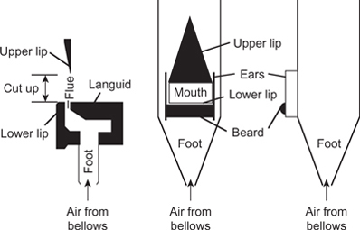
Figure 4.13 The main elements of the sound source in organ flue pipes based on a wooden flue pipe (left) and additional features found on some metal pipes (center and left).
Air enters the pipe from the organ bellows via the foot and a thin sheet of air emerges from the flue. If the upper lip were not present, the air emerging from the flue would be heard as noise. This indicates that the airstream is turbulent. A similar effect can be observed if you form the mouth shape for the “ff” in far, in which the bottom lip is placed in contact with the upper teeth to produce the “ff” sound. The airflow is turbulent, producing the acoustic noise which can be clearly heard. If the airstream flow rate is reduced, there is an air velocity below which turbulent flow ceases and acoustic noise is no longer heard. At this point the airflow has become smooth or “laminar.” Turbulent airflow is the mechanism responsible for the non-pitched sounds in speech such as the “sh” in shoe and the “ss” in sea, for which waveforms and spectra are shown in Figure 3.9.
When a wedge-like obstruction is placed in the airstream emerging from the flue a definite sound is heard known as an “edgetone.” Hall suggests a method for demonstrating this by placing a thin card in front of the mouth and blowing on its edge. Researchers are not fully agreed on the mechanism which underlies the sound source in flues. The preferred explanation is illustrated in Figure 4.14, and it is described in relation to the sequence of snapshots in the figure as follows. Air flows to one side of the obstruction, causing a local increase in pressure on that side of it. This local pressure increase causes air in its local vicinity to be moved out of the way, and some finds its way in a circular motion into the pipe via the mouth. This has the effect of “bending” the main stream of air increasingly, until it flips into the pipe. The process repeats itself, only this time the local pressure increase causes air to move in a circular motion out of the pipe via the mouth, gradually bending the main airstream until it flips outside the pipe again. The cycle then repeats providing a periodic sound source to the pipe itself. This process is sometimes referred to as a vibrating “air reed” due to the regular flipping to and fro of the airstream.

Figure 4.14 Sequence of events to illustrate the sound source mechanism in a flue organ pipe.
The f0 of the pulses generated by this air reed mechanism in the absence of a pipe resonator is directly proportional to the airflow velocity from the flue, and inversely proportional to the length of the cut-up:
![]()
where ∝ | means "is proportional to" |
f0 = | fundamental frequency of air reed oscillation in absence of pipe resonator |
vj = | airflow velocity |
and Lcut-put = | length of cut-up |
In other words, f0 can be raised by either increasing the airflow velocity or reducing the cut-up. As the airflow velocity is increased or the cut-up size is decreased, there comes a point where the f0 jumps up in value. This effect can be observed in the presence of a resonator with respect to increasing the airflow velocity by blowing with an increasing flow rate into a recorder (or if available, a flue organ pipe). It is often referred to as an “overblown” mode.
The acoustic nature of the sound source in flues is set by the pipe voicer, whose job it is to determine the overall sound from individual pipes and to establish an even tone across complete ranks of pipes. The following comments on the voicer’s art in relation to the sound source in flue pipes are summarized from Norman and Norman (1980), who give the main modifications made by the voicer in order of application as:
- adjusting the cut-up;
- “nicking” the languid and lower lip;
- adjusting languid height with respect to that of the lower lip.
Adjusting the cut-up needs to be done accurately to achieve an even tone across a rank of pipes. This is achieved on metal pipes by using a sharp, short, thick-bladed knife. A high cut-up produces a louder and more “hollow” sound, and a lower cut-up gives a softer and “edgier” sound. The higher the cut-up, the greater the airflow required from the foot. However, the higher the airflow, the less prompt the speech of the pipe.
Nicking relates to a series of small nicks that are made in the approximating edges of the languid and the upper lip. This has the effect of reducing the high-frequency components in the sound source spectrum and giving the pipe a smoother, but slower, onset to its speech. More nicking is customarily applied to pipes which are heavily blown. A pipe which is not nicked has a characteristic consonantal attack to its sound, sometimes referred to as a “chiff.” A current trend in organ voicing is the use of less or no nicking in order to take advantage of the onset chiff musically to give increased clarity to notes, particularly in contrapuntal music (e.g., Hurford, 1994).
The height of the languid is fixed at manufacture for wooden pipes, but it can be altered for metal pipes. The languid controls, in part, the direction of the air flowing from the flue. If it is too high, the pipe will be slow to speak and may not speak at all if the air misses the upper lip completely. If it is too low the pipe will speak too quickly, or speak in an uncontrolled manner. A pipe is adjusted to speak more rapidly if it is set to speak with a consonantal chiff by means of little or no nicking. Narrow scaled pipes (small diameter compared with the length) usually have a “stringy” tone color and often have ears added (see Figure 4.12) which stabilize air reed oscillation. Some bass pipes also have a wooden roller or “beard” placed between the ears to aid prompt pipe speech.
4.3.2 Sound Modifiers in Organ Flue Pipes
The sound modifier in an organ flue pipe is the main body of the pipe itself, or its “resonator” (see Figure 4.12). Organ pipe resonators are made in a variety of shapes developed over a number of years to achieve subtleties of tone color, but the most straightforward to consider are resonators whose dimensions do not vary along their length, or resonators of “uniform cross-section.” Pipes made of metal are usually round in cross-section and those made of wood are generally square (some builders make triangular wooden pipes, partly to save on raw material). These shapes arise mainly from ease of construction with the material involved.
There are two basic types of organ flue pipe: those that are open and those that are stopped at the end farthest from the flue itself (see Figure 4.12). The flue end of the pipe is acoustically equivalent to an open end. Thus the open flue pipe is acoustically open at both ends, and the stopped flue pipe is acoustically open at one end and closed at the other. The air reed sound source mechanism in flue pipes as illustrated in Figure 4.14 launches a pulse of acoustic energy into the pipe. When a compression (positive amplitude) pulse of sound pressure energy is launched into a pipe, for example at the instant in the air reed cycle illustrated in the lower-right snapshot in Figure 4.14, it travels down the pipe at the velocity of sound as a compression pulse.
When the compression pulse reaches the far end of the pipe, it is reflected in one of the two ways described in the “standing waves” section of Chapter 1 (Section 1.5.7), depending on whether the end is open or closed. At a closed end there is a pressure antinode and a compression pulse is reflected back down the pipe. At an open end there is a pressure node and a compression pulse is reflected back as a rarefaction pulse to maintain atmospheric pressure at the open end of the pipe. Similarly, a rarefaction pulse arriving at a closed end is reflected back as a rarefaction pulse, but as a compression pulse when reflected from an open end. All four conditions are illustrated in Figure 4.15.

Figure 4.15 The reflected pulses resulting from a compression (upper) and rarefaction (lower) pulse arriving at an open (left) and a stopped (right) end of a pipe of uniform cross-section. (Note: Time axes are marked in equal arbitrary units.)
When the action of the resonator on the air reed sound source in a flue organ pipe is considered (see Figure 4.14), it is found that the f0 of air reed vibration is entirely controlled by: (a) the length of the resonator, and (b) whether the pipe is open or stopped. This dependence of the f0 of the air reed vibration can be appreciated by considering the arrival and departure of pulses at each end of the open and the stopped pipes.
Figure 4.16 shows a sequence of snapshots of pressure pulses generated by the air reed traveling down an open pipe of length Lo (left) and a stopped pipe of length Ls (right), and how they drive the vibration of the air reed. (Air reed vibration is illustrated in a manner similar to that used in Figure 4.14.) The figure shows pulses moving from left to right in the upper third of each pipe, those moving from right to left in the center third, and the summed pressure in the lower third. A time axis with arbitrary but equal units is marked in the figure to show equal time intervals. The pulses travel an equal distance in each frame of the figure since an acoustic pulse moves at a constant velocity. The flue end of the pipe acts as an open end in terms of the manner in which pulses are reflected (see Figure 4.15). At every instant when a pulse arrives and is reflected from the flue end, the air reed is flipped from inside to outside when a compression pulse arrives and is reflected as a rarefaction pulse, and vice versa when a rarefaction pulse arrives. This can be observed in Figure 4.16.

Figure 4.16 Pulses traveling in open (left) and stopped (right) pipes when they drive an air reed sound source. (Note: Time axis is marked in equal arbitrary time units; pulses traveling left to right are shown in the upper part of each pipe, those going right to left are shown in the center, and the sum is shown in the lower part.)
For the open pipe, the sequence in the figure begins with a compression pulse being launched into the pipe, and another compression pulse just leaving the open end (the presence of this second pulse will be explained shortly). The next snapshot (2) shows the instant when these two pulses reach the center of the pipe, their summed pressure being a maximum at this point. The pulses effectively travel through each other and emerge with their original identities due to “superposition” (see Chapter 1). In the third snapshot the compression pulse is being reflected from the open end of the pipe as a rarefaction pulse, and the air reed flips outside the pipe, generating a rarefaction pulse. (This may seem strange at first, but it is a necessary consequence of the event happening in the fifth snapshot.) The fourth snapshot shows two rarefactions at the center giving a summed pressure which is a minimum at this instant of twice the rarefaction pulse amplitude. In the fifth snapshot, when the rarefaction pulse is reflected from the flue end as a compression pulse, the air reed is flipped from outside to inside the pipe. One cycle is complete at this point since events in the fifth and first snapshots are similar. (A second cycle is illustrated on the right-hand side of Figure 4.1 to enable comparison with events in the stopped pipe.)
The fundamental period for the open pipe is the time taken to complete a complete cycle (i.e., the time between a compression pulse leaving the flue end of the pipe and the next compression pulse leaving the flue end of the pipe). In terms of Figure 4.16 it is four time frames (snapshot one Stopped pipe to snapshot five), being the time taken for the pulse to travel down to the other end and back (see Figure 4.15), or twice the open pipe length:
![]()
where T0(open) = | fundamental period of open pipe |
Lo = | lenght of the open pipe |
and c = | velocity of sound |
The f0 value for the open pipe is therefore:

In the stopped pipe, the sequence in Figure 4.15 again begins with a compression pulse being launched into the pipe, but there is no second pulse. Snapshot two shows the instant when the pulses reach the center of the pipe, and the third snapshot the instant when the compression pulse is reflected from the stopped end as a compression pulse (see Figure 4.15) and the summed pressure is a maximum for the cycle of twice the amplitude of the compression pulse. The fourth snapshot shows the compression pulse at the center and in the fifth, the compression pulse is reflected from the flue end as a rarefaction pulse, flipping the air reed from inside to outside the pipe. The sixth snapshot shows the rarefaction pulse halfway down the pipe and the seventh shows its reflection as a rarefaction pulse from the stopped end when the summed pressure there is the minimum for the cycle of twice the amplitude of the rarefaction pulse. The eighth snapshot shows the rarefaction pulse halfway back to the flue end and, by the ninth, one cycle is complete, since events in the ninth and first snapshots are the same.
It is immediately clear that one cycle for the stopped pipe takes twice as long as one cycle for the open pipe if the pipe lengths are equal (ignoring a small end correction which has to be applied in practice). Its fundamental period is therefore double that for the open pipe, and its f0 is therefore half that for the open pipe, or an octave lower. This can be quantified by considering that the time taken to complete a complete cycle is the time required for the pulse to travel to the other end of the pipe and back twice, or four times the stopped pipe length (see Figure 4.15):
![]()
where T0(stopped) = | fundamental period of open pipe |
Ls = | lenght of the stopped pipe |
and c = | velocity of sound |
Therefore:

Example 4.2
If an open pipe and a stopped pipe are the same length, what is the relationship between their f0 values?
Let (Ls = Lo = L) and substitute into Equations 4.5 and 4.6:

Therefore:
![]()
Therefore f0(stopped) is an octave lower than f0(open) (frequency ratio 1:2).
The natural modes of a pipe are constrained as described in the “standing waves” section of Chapter 1. Equation 1.35 gives the frequencies of the modes of an open pipe and Equation 1.36 gives the frequencies of the modes of a stopped pipe. In both equations, the velocity is the velocity of sound (c).
The frequency of the first mode of the open pipe is given by Equation 1.30 when (n = 1):

which is the same value obtained in Equation 4.5 by considering pulses in the open pipe. Using Equation 1.35, the frequencies of the other modes can be expressed in terms of its f0 value as follows:
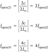
In general:
![]()
The modes of the open pipe are thus all harmonically related and all harmonics are present. The musical intervals between the modes can be read from Figure 3.3.
The frequency of the fundamental mode of the stopped pipe is given by Equation 1.36 when (n = 1):
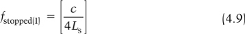
This is the same value obtained in Equation 4.6 by considering pulses in the stopped pipe. The frequencies of the other stopped pipe modes can be expressed in terms of its f stopped using Equation 1.36 as follows:

![]()
where n = 1, 2, 3, 4, …
Thus the modes of the stopped pipe are harmonically related, but only the odd-numbered harmonics are present. The musical intervals between the modes can be read from Figure 3.3.
In open and stopped pipes the pipe’s resonator acts as the sound modifier and the sound source is the air reed. The nature of the spectrum of the air reed source depends on the detailed shape of the pulses launched into the pipe, which in turn depends on the pipe’s voicing summarized above. If a pipe is overblown, its f0 jumps to the next higher mode that the resonator can support: up one octave to the second harmonic for an open pipe, and up an octave and a fifth to the third harmonic for the stopped pipe.
The length of the resonator controls the f0 of the air reed (see Figure 4.15) and the natural modes of the pipe are the frequencies that the pipe can support in its output. The amplitude relationship between the pipe modes is governed by the material from which the pipe is constructed and the diameter of the pipe with respect to its length. In particular, wide pipes tend to be weak in upper harmonics. Organ pipes are tuned by adjusting the length of their resonators. In open pipes this is usually done nowadays by means of a tuning slide fitted round the outside of the pipe at the open end, and for stopped pipes by moving the stopper (see Figure 4.12).
A stopped organ pipe has an f0 value which is an octave below that of an open organ pipe (Example 4.2), and, where space is limited in an organ, stopped pipes are often used in the bass register and played by the pedals. However, the trade-off is between the physical space saved and the acoustic result in that only the odd-numbered harmonics are supported. Figure 4.17 illustrates this with waveforms and spectra for middle C played on a gedackt 8″ and a principal 8′ (Section 5.4 describes organ stop footages: 8′, 4′, etc.). The gedackt stop has stopped wooden pipes, and the spectrum clearly shows the presence of odd harmonics only, in particular the first, third and fifth. The principal stop consists of open metal pipes, and odd and even harmonics exist in its output spectrum. Although the pitch of these stops is equivalent, and they are therefore both labeled 8′, the stopped gedackt pipe is half the length of the open principal pipe.

Figure 4.17 Waveforms and spectra for middle C (C4) played on a gedackt 8′ (stopped flue) and a principal 8′ (open flue).
4.3.3 Woodwind Flue Instruments
Other musical instruments which have an air reed sound source include the recorder and the flute. Useful additional material on woodwind flue instruments can be found in Benade (1976) and Fletcher and Rossing (1999). The air reed action is controlled by oscillatory changes in flow of air in and out of the flue (see Figure 4.16), often referred to as a “flow-controlled valve,” and therefore there must be a velocity antinode and a pressure node. Hence the flue end of the pipe is acting as an open end, and woodwind flue instruments act acoustically as pipes open at both ends (see Figure 4.18).

Figure 4.18 The first four pressure and velocity modes of an open and a stopped pipe of uniform cross-section. (Note: The plots show maximum and minimum amplitudes of pressure and velocity.)
Players are able to play a number of different notes on the same instrument by changing the effective acoustic length of the resonator. This can be achieved, for example, by means of the sliding piston associated with a swanee whistle or more commonly when particular notes are required, by covering and uncovering holes in the pipe walls known as “finger holes.” A hole in a pipe will act in an acoustically similar manner to an open pipe end (pressure node, velocity antinode). The extent to which it does this is determined by the diameter of the hole with respect to the pipe diameter. When this is large with respect to the pipe diameter, as in the flute, the uncovered hole acts acoustically as if the pipe had an open end at that position. Smaller finger holes result acoustically in the effective open end being further down the pipe (away from the flue end). This is an important factor in the practical design of bass instruments with long resonators since it can enable the finger holes to be placed within the physical reach of a player’s hands. It does, however, have an important consequence on the frequency relationship between the modes, and this is explored in detail below in connection with woodwind reed instruments. The other way to give a player control over finger holes which are out of reach, for example on a flute, is by providing each hole with a pad controlled by a key mechanism of rods and levers operated by the player’s fingers to close or open the hole (depending on whether the hole is normally open or closed by default).
In general, a row of finger holes is gradually uncovered to effectively shorten the acoustic length of the resonator as an ascending scale is played. Occasionally some cross-fingering is used in instruments with small holes or small pairs of holes such as the recorder as illustrated in Figure 4.19. Here, the pressure node is further away from the flue than the first uncovered hole itself such that the state of other holes beyond it will affect its position. The figure shows typical fingerings used to play a two octave C major scale on a descant or tenor recorder. Hole fingerings are available to enable notes to be played which cover a full chromatic scale across one octave. To play a second octave on woodwind flue instruments, such as the recorder or flute, the flue is overblown. Since these instruments are acoustically open at both ends, the overblown flue jumps to the second mode which is one octave higher than the first (see Equation 4.8 and Figure 3.3). The finger holes can be reused to play the notes of the second octave.

Figure 4.19 Fingering chart for recorders in C (descants and tenors).
Once an octave and a fifth above the bottom note has been reached, the flue can be over-blown to the third mode (an octave and a fifth above the first mode) and the fingering can be started again to ascend higher. The fourth mode is available at the start of the third octave, and so on. Overblowing is supported in instruments such as the recorder by opening a small “register” or “vent” hole which is positioned such that it is at the pressure antinode for unwanted modes and these modes will be suppressed. The register hole marked in Figure 4.19 is a small hole on the back of the instrument which is controlled by the thumb of the left hand which either covers it completely, half covers it by pressing the thumb nail end-on against it, or uncovers it completely. To suppress the first mode in this way without affecting the second, this hole should be drilled in a position where the undesired mode has a pressure maximum. When all the tone holes are covered, this would be exactly halfway down the resonator—a point where the first mode has a pressure maximum and is therefore reduced, but the second mode has a pressure node and is therefore unaffected (see Figure 4.18). Register holes can be placed at other positions to enable overblowing to different modes. In practice, register holes may be set in compromise positions because they have to support all the notes available in that register, for which the effective pipe length is altered by uncovering tone holes.
A flute has a playing range between B3 and D7, and the piccolo sounds one octave higher between B4 and D8 (see Figure 4.3). Flute and piccolo players can control the stability of the overblown modes by adjusting their lip position with respect to the embouchure hole as illustrated in Figure 4.20. The air reed mechanism can be compared with that of flue organ pipes illustrated in Figures 4.13 and 4.14 as well as the associated discussion relating to organ pipe voicing. The flautist is able to adjust the distance between the flue outlet (the player’s lips) and the edge of the mouthpiece, marked as the “cut-up” in the figure, a term borrowed from organ nomenclature (see Figure 4.13), by rolling the flute as indicated by the double-ended arrow. In addition, the airflow velocity can be varied as well as the fine detailed nature of the airstream dimensions by adjusting the shape, width and height of the opening between the lips. The flautist therefore has direct control over the stability of the overblown modes (Equation 4.4).

Figure 4.20 Illustration of lip to embouchure adjustments available to a flautist.
4.3.4 Sound Source in Organ Reed Pipes
The basic components of an organ reed pipe are shown in Figure 4.12. The sound source results from the vibrations of the reed, which is slightly larger than the shallot opening, against the edges of the shallot. Very occasionally, organ reeds make use of “free reeds,” which are cut smaller than the shallot opening and move in and out of the shallot without coming into contact with its edges. In its rest position, as illustrated in Figure 4.12, there is a gap between the reed and shallot, enabled by the slight curve in the reed itself. The vibrating length of the reed is governed by the position of the “tuning wire,” or “tuning spring,” which can be nudged up or down to make the vibrating length longer or shorter, accordingly lowering or raising the f0 of the reed vibration.
The reed vibrates when the stop is selected and a key on the appropriate keyboard is pressed. This causes air to enter the boot and flow past the open reed via the shallot to the resonator. The gap between the reed and shallot is narrow, and for air to flow there must be a higher pressure in the boot than in the shallot, which tends to close the reed fractionally, resulting in the gap between the reed and shallot being narrowed. When the gap is narrowed, the airflow rate is increased and the pressure difference which supports this higher airflow is raised. The increase in pressure difference exerts a slightly greater closing force on the reed, and this series of events continues, accelerating the reed towards the shallot until it hits the edge of the shallot, closing the gap completely and rapidly.
The reed is springy and once the gap is closed and the flow has dropped to zero, the reed’s restoring force causes the reed to spring back towards its equilibrium position, opening the gap. The reed overshoots its equilibrium position, stops, and returns towards the shallot, in a manner similar to its vibration if it had been displaced from its equilibrium position and released by hand. Airflow is restored via the shallot and the cycle repeats.
In the absence of a resonator, the reed would vibrate at its natural frequency. This is the frequency at which it would vibrate if it were plucked. If a plucked reed continues to vibrate for a long time, then it has a strong tendency to vibrate at a frequency within a narrow range but, if it vibrates for a short time, there is a wide range of frequencies over which it is able to vibrate. This effect is illustrated in Figure 4.21. This difference is exhibited depending on the material from which the reed is made and how it is supported. A reed which vibrates over a narrow frequency range is usually made from brass and supported rigidly, and is known as a “hard” reed. A reed which vibrates over a wide range might be made from cane or plastic, held in a pliable support, and known as a “soft” reed. As shown in the figure, the natural period (TN) is related to the natural frequency (FN) as:

Figure 4.21 Time (left) and frequency (right) responses of hard (upper) and soft (lower) reeds when plucked. Natural frequency (FN) and natural period (TN) are shown.
![]()
A reed vibrating against a shallot shuts off the flow of air rapidly and totally, and the consequent acoustic pressure variations are the sound source provided to the resonator. The rapid shutting off of the airflow produces a rapid, instantaneous drop in acoustic pressure within the shallot (as air flowing fast into the shallot is suddenly cut off). A rapid amplitude change in a waveform indicates a relatively high proportion of high harmonics are present. The exact nature of the sound source spectrum depends on the particular reed, shallot and bellows pressure being considered. Free reeds which do not make contact with a shallot, as found for example in a harmonica or harmonium, do not produce as high a proportion of high harmonics since the airflow is never completely shut off.
4.3.5 Sound Modifiers in Organ Reed Pipes
All reed pipes have resonators. The effect of a resonator has already been described and illustrated in Figure 4.16 in connection with air reeds. The same principles apply to reed pipes, but there is a major difference in that the shallot end of the resonator acts as a stopped end (as opposed to an open end as in the case of a flue). This is because during reed vibration, the pipe is either closed completely at the shallot end (when the reed is in contact with the shallot) or open with a very small aperture compared with the pipe diameter.
Organ reed pipes have hard reeds, which have a narrow natural frequency range (see Figure 4.21). Unlike the air reed, the presence of a resonator does not control the frequency of vibration of the hard reed. The sound-modifying effect of the resonator is based on the modes it supports (see Figure 4.18), bearing in mind the closed end at the shallot. Because the reed itself fixes the f0 of the pipe, the resonator does not need to reinforce the fundamental and fractional length resonators are sometimes used to support only the higher harmonics. Figure 4.22 shows waveforms and spectra for middle C (C4) played on a hautbois 8′, or oboe 8′, and a trompette 8′, or trumpet 8′. Both spectra exhibit an overall peak around the sixth/seventh harmonic. For the trompette this peak is quite broad with the odd harmonics dominating the even ones up to the tenth harmonic, probably a feature of its resonator shape. The hautbois spectrum exhibits more dips in the spectrum than the trompette—these are all features which characterize the sounds of different instruments as being different.

Figure 4.22 Waveform and spectra for middle C (C4) played on a hautbois 8′ and a trompette 8′.
4.3.6 Woodwind Reed Instruments
Woodwind reed instruments make use of either a single or a double vibrating reed sound source which controls the flow of air from the player’s lungs to the instrument. The action of a vibrating reed at the end of a pipe is controlled as a function of the relative air pressure on either side of it in terms of when it opens and closes. It is therefore usually described as a pressure-controlled valve, and the reed end of the pipe acts as a stopped end (pressure antinode and velocity node—see Figure 4.18). Note that although the reed opens and closes such that airflow is not always zero, the reed opening is very much smaller than the pipe diameter elsewhere, making a stopped end reasonable. This is in direct contrast to the air reed in woodwind flue instruments such as the flute and recorder (see above), which, as a flow-controlled valve, provides a velocity antinode and a pressure node, and where the flue end of the pipe acts as an open end (see Figure 4.18).
Soft reeds are employed in woodwind reed instruments which can vibrate over a wide frequency range (see Figure 4.21). The reeds in clarinets and saxophones are single reeds which can close against the edge of the mouthpiece as in organ reed pipes where they vibrate against their shallots. The oboe and bassoon on the other hand use double reeds, but the basic opening and closing action of the sound source mechanism is the same.
Woodwind reed instruments have resonators whose modal behavior is crucial to the operation of these instruments and provide the sound modifier function. Woodwind instruments incorporate finger holes to enable chromatic scales to be played from the first mode to the second mode when the fingering can be used again as the reed excites the second mode. These mode changes continue up the chromatic scale to cover the full playing range of the instrument (see Figure 4.3). Clearly it is essential that the modes of the resonator retain their frequency ratios relative to each other as the tone holes are opened, or else the instrument’s tuning will be adversely affected as higher modes are reached. Benade (1976) summarizes this effect and indicates the resulting constraint as follows:
Preserving a constant frequency ratio between the vibrational modes as the holes are opened is essential in all woodwinds and provides a limitation on the types of air column (often referred to as the bore) that are musically useful.
The musically useful bores in this context are based on tubing that is either cylindrical, as in the clarinet, or conical as in the oboe, cor Anglais, and members of the saxophone and bassoon families. The cylindrical resonator of a clarinet acts as a pipe that is stopped at the reed end (see above) but is open at the other. Odd numbered modes only are supported by such a resonator (see Figure 4.18), and its f0 is an octave lower (see Example 4.2) than that of an instrument with a similar length pipe which is open at both ends, such as a flute (see Figure 4.3). The first overblown mode of a clarinet is therefore the third mode, an interval of an octave and a fifth (see Figure 3.3), and therefore, unlike a flute or recorder, it has to have sufficient holes to enable at least 19 chromatic notes to be fingered within the first mode prior to transition to the second.
Conical resonators that are stopped at the reed end and open at the other support all modes in a harmonically related manner. Taylor (1976) gives a description of this effect as follows:
Suppose by some means we can start a compression from the narrow end; the pipe will behave just as our pipe open at both ends until the rarefaction has returned to the start. Now, because the pipe has shrunk to a very small bore, the speed of the wave slows down and no real reflection occurs…. The result is that we need only consider one journey out and one back regardless of whether the pipe is open or closed at the narrow end…. The conical pipe will behave something like a pipe open at both ends as far as its modes are concerned.
The conical resonator therefore supports all modes, and the overblown mode of instruments with conical resonators, such as the oboe, cor Anglais, bassoon and saxophone family, is therefore to the second mode, or up an octave. Sufficient holes are therefore required for at least 12 chromatic notes to be fingered to enable the player to arrive at the second mode from the first.
The presence of a sequence of open tone holes in a pipe resonator of any shape is described by Benade (1976) as a tone-hole lattice. The effective acoustical end-point of the pipe varies slightly as a function of frequency when there is a tone-hole lattice, and therefore the effective pipe length is somewhat different for each mode. A pipe with a tone-hole lattice is acoustically shorter for low-frequency standing wave modes compared with higher-frequency modes, and therefore the higher-frequency modes are increasingly lowered slightly in frequency (lengthening the wavelength lowers the frequency). Above a particular frequency, described by Benade (1976) as the open-holes lattice cut-off frequency (given as around 350–500 Hz for quality bassoons, 1500 Hz for quality clarinets and between 1100 and 1500 Hz for quality oboes), sound waves are not reflected due to the presence of the lattice. Benade notes that this has a direct effect on the perceived timbre of woodwind instruments, correlating well with descriptions such as bright or dark given to instruments by players. It should also be noted that holes that are closed modify the acoustic properties of the pipe also, and this can be effectively modeled as a slight increase in pipe diameter at the position of the tone hole. The resulting acoustic change is considered below.
In order to compensate for these slight variations in the frequencies of the modes produced by the presence of open and closed tone holes, alterations can be made to the shape of the pipe. These might include flaring the open end, adding a tapered section, or small local voicing adjustments by enlarging or constricting the pipe, which on a wooden instrument can be achieved by reaming out or adding wax respectively (e.g., Nederveen, 1969). The acoustic effect on individual pipe mode frequencies of either enlarging or constricting the size of the pipe depends directly on the mode’s distribution of standing wave pressure nodes and antinodes (or velocity antinodes and nodes respectively). The main effect of a constriction in relation to pressure antinodes (velocity nodes) is as follows (Kent and Read, 1992):
- A constriction near a pressure node (velocity antinode) lowers that mode’s frequency.
- A constriction near a pressure antinode (velocity node) raises that mode’s frequency.
A constriction at a pressure node (velocity antinode) has the effect of reducing the flow at the constriction since the local pressure difference across the constriction has not changed. Benade (1976) notes that this is equivalent to raising the local air density, and the discussion in Chapter 1 indicates that this will result in a lowering of the velocity of sound (see Equation 1.1) and therefore a lowering in the mode frequency (see Equations 4.7 and 4.9). A constriction at a pressure antinode (velocity node), on the other hand, provides a local rise in acoustic pressure which produces a greater opposition to local airflow of the sound waves that combine to produce the standing wave modes. This is equivalent to raising the local springiness in the medium (air), which is shown in Chapter 1 to be equivalent for air in Young’s modulus (Egas), which raises the velocity of sound (see Equation 1.5) and therefore raises the mode frequency (see Equations 4.7 and 4.9). By the same token, the effect of locally enlarging a pipe will be exactly opposite to that of constricting it.
Knowledge of the position of the pressure and velocity nodes and antinodes for the standing wave modes in a pipe therefore allows the effect on the mode frequencies of a local constriction or enlargement of a pipe to be predicted. Figure 4.23 shows the potential mode frequency variation for the first three modes of a cylindrical stopped pipe that could be caused by a constriction or enlargement at any point along its length. (The equivalent diagram for a cylindrical pipe open at both ends could be readily produced with reference to Figures 4.18 and 4.23; this is left as an exercise for the interested reader.)
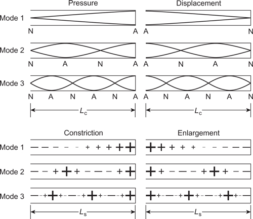
Figure 4.23 The effect of locally constricting or enlarging a stopped pipe on the frequencies of its first three modes: “+” indicates raised modal frequency, “–” indicates lowered modal frequency, and the magnitude of the change is indicated by the size of the “+” or “−” signs. The first three pressure and velocity modes of a stopped pipe are shown for reference: “N” and “A” indicate node and antinode positions respectively
The upper part of Figure 4.23 (taken from Figure 4.18) indicates the pressure and velocity node and antinode positions for the first three standing wave modes. The lower part of the figure exhibits plus and minus signs to indicate where that particular mode’s frequency would be raised or lowered respectively by a local constriction or enlargement at that position in the pipe. The size of the signs indicates the sensitivity of the frequency variation based on how close the constriction is to the mode’s pressure/velocity nodes and antinodes shown in the upper part of the figure. For example, a constriction close to the closed end of a cylindrical pipe will raise the frequencies of all modes since there is a pressure antinode at a closed end, whereas an enlargement at that position would lower the frequencies of all modes. However, if a constriction or enlargement were made one-third the way along a stopped cylindrical pipe from the closed end, the frequencies of the first and third modes would be raised somewhat, but that of the second would be lowered maximally. By creating local constrictions or enlargements, the skilled maker is able to set up a woodwind instrument to compensate for the presence of tone holes such that the modes remain close to being in integer frequency ratios over the playing range of the instrument.
Figure 4.24 shows waveforms and spectra for the note middle C played on a clarinet and a tenor saxophone. The saxophone spectrum contains all harmonics since its resonator is conical. The clarinet spectrum exhibits the odd harmonics clearly as its resonator is a cylindrical pipe closed at one end (see Figure 4.18), but there is also energy clearly visible in some of the even harmonics. Although the resonator itself does not support the even modes, the spectrum of the sound source does contain all harmonics (the saxophone and the clarinet are both single reed instruments). Therefore some energy will be radiated by the clarinet at even harmonics.

Figure 4.24 Waveforms and spectra for middle C (C4) played on a clarinet and a tenor saxophone.
Sundberg (1989) summarizes this effect for the clarinet as follows:
This means that the even-numbered modes are not welcome in the resonator…. A common misunderstanding is that these partials are all but missing in the spectrum. The truth is that the second partial may be about 40 dB below the fundamental, so it hardly contributes to the timbre. Higher up in the spectrum the differences between odd- and even-numbered neighbors are smaller. Further … the differences can be found only for the instruments’ lower tones.
This description is in accord with the spectrum in Figure 4.24, where the amplitude of the second harmonic is approximately 40 dB below that of the fundamental, and the odd/even differences become less with increased frequency.
The brass instrument family has an interesting history from early instruments derived from natural tube structures such as the horns of animals, seashells and plant stems, through a variety of wooden and metal instruments to today’s metal brass orchestral family (e.g., Campbell and Greated, 1998; Fletcher and Rossing, 1999). The sound source in all brass instruments is the vibrating lips of the player in the mouthpiece. They form a double soft reed, but the player has the possibility of adjusting the physical properties of the double reed by lip tension and shape. The lips act as a pressure-controlled valve in the manner described in relation to the woodwind reed sound source, and therefore the mouthpiece end of the instrument acts acoustically as a stopped end (pressure antinode and velocity node—see Figure 4.18).
The double reed action of the lips can be illustrated if the lips are held slightly apart, and air is blown between them. For slow airflow rates nothing is heard, but, as the airflow is increased, acoustic noise is heard as the airflow becomes turbulent. If the flow is increased further, the lips will vibrate together as a double reed. This vibration is sustained by the physical vibrational properties of the lips themselves, and an effect known as the “Bernoulli effect.”
As air flows past a constriction, in this case the lips, its velocity increases. The Bernoulli effect is based on the fact that at all points the sum of the energy of motion, or “kinetic” energy, plus the pressure energy, or “potential” energy, must be constant at all points along the tube. Figure 4.25 illustrates this effect in a tube with a flexible constriction. Airflow direction is represented by the lines with arrows, and the velocity of airflow is represented by the distance between these lines. Since airflow increases as it flows through the constriction, the kinetic energy increases. In order to satisfy the Bernoulli principle that the total energy remains constant, the potential energy or the pressure at the point of constriction must therefore reduce. This means that the force on the tube walls is lower at the point of constriction.
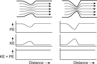
Figure 4.25 An illustration of the Bernoulli effect (potential energy + kinetic energy = a constant) in a tube with a constriction. (Note: Lines with arrows represent airflow direction, and the distance between them is proportional to the airflow velocity. PE = potential energy; KE = kinetic energy.)
If the wall material at the point of constriction is elastic and the force exerted by the Bernoulli effect is sufficient to move the walls’ mass (such as the brass player’s lips) from its rest (equilibrium) position, then the walls are sucked together a little (compare the right- and left-hand illustrations in the figure). Now the kinetic energy (airflow velocity) becomes greater because the constriction is narrower; thus the potential energy (pressure) must reduce some more to compensate (compare the graphs in the figure), and the walls of the tube are sucked together with greater force. Therefore the walls are accelerated together as the constriction narrows until they smack together, cutting off the airflow. The air pressure in the tube tends to push the constriction apart, as does the natural tendency of the walls to return to their equilibrium position. Like two displaced pendulums, the walls move past their equilibrium position, stop and return towards each other, and the Bernoulli effect accelerates them together again. The oscillation of the walls will be sustained by the airflow, and the vibration will be regular if the two walls at the point of constriction have similar masses and tensions, such as the lips.
The lip reed vibration is supported by the resonator of the brass instrument formed by a length of tubing attached to a mouthpiece. Some mechanism is provided to enable the player to vary the length of the tube, which was done originally, for example, in the horn family by adding different lengths of tubing or “crooks” by hand. Nowadays this is accomplished by means of a sliding section as in the trombone or by adding extra lengths of tubing by means of valves. The tube profile in the region of the trombone slide or tunable valve mechanism has to be cylindrical in order for slides to function.
All brass instruments consist of four sections (see Figure 4.26): mouthpiece, a tapered mouthpipe, a main pipe fitted with slide or valves which is cylindrical (e.g., trumpet, French horn, trombone) or conical (e.g., cornet, flugelhorn, baritone horn, tuba), and a flared bell (Benade, 1976; Hall, 2001). If a brass instrument consisted only of a conical main pipe, all modes would be supported (see discussion on woodwind reed instruments above), but, if it were cylindrical, it acts as a stopped pipe due to the pressure-controlled action of the lip reed and therefore only odd-numbered modes would be supported (see Figure 4.18). However, instruments in the brass family support almost all modes which are essentially harmonically related due to the acoustic action of the addition of the mouthpiece and bell.

Figure 4.26 Basic sections of a brass instrument.
The bell modifies as a function of frequency the manner in which the open end of the pipe acts as a reflector of sound waves arriving there from within the pipe. A detailed discussion is provided by Benade (1976) from which a summary is given here. Lower-frequency components are reflected back into the instrument from the narrower part of the bell while higher-frequency components are reflected from the wider regions of the bell. Frequencies higher than a cut-off frequency determined by the diameter of the outer edge of the bell (approximately 1500 Hz for a trumpet) are not reflected appreciably by the bell. Adding a bell to the main bore of the instrument has the effect of making the effective pipe length longer with increasing frequency. The frequency relationship between the modes of the stopped cylindrical pipe (odd-numbered modes only: 1f, 3f, 5f, 7f, etc.) will therefore be altered such that they are brought closer together in frequency. This effect is greater for the first few modes of the series.
The addition of a mouthpiece at the other end of the main bore also affects the frequency of some of the modes. The mouthpiece consists of a cup-shaped cavity which communicates via a small aperture with a short conical pipe. The mouthpiece has a resonant frequency associated with it, which is generally in the region of 850 Hz for a trumpet, which is otherwise known as the “popping frequency” since it can be heard by slapping its lip contact end on the flattened palm of one hand (Benade, 1976). The addition of a mouthpiece effectively extends the overall pipe length by an increasing amount. Benade notes that this effect “is a steady increase nearly to the top of the instrument’s playing range,” and that a mouthpiece with a “lower popping frequency will show a greater total change in effective length as one goes up in frequency” (Benade, 1976, p. 416). This pipe length extension caused by adding a mouthpiece therefore has a greater downwards frequency shifting effect on the higher compared with the lower modes.
In a complete brass instrument, it is possible through the use of an appropriately shaped bell, mouthpiece and mouthpipe to construct an instrument whose modes are frequency shifted from the odd only modes of a stopped cylindrical pipe to being very close to a complete harmonic series. In practice, the result is a harmonic series where all modes are within a few per cent of being integer multiples of a common lower-frequency value except for the first mode itself, which is well below that lower-frequency value common to the higher modes and therefore it is not harmonically related to them. The effects of the addition of the bell and mouthpiece/mouthpipe on the individual lowest six modes are broadly as summarized in Figure 4.27. Here the odd-numbered modal frequencies of the stopped cylindrical pipe are denoted as integer multiples of frequency “f,” and the resulting brass instrument modal frequencies are shown as multiples of another frequency “F.”

Figure 4.27 Brass instrument mode frequency modification to stopped cylindrical pipe by the addition of mouthpiece/mouthpipe and bell.
The second mode is therefore the lowest musically usable mode available in a brass instrument (note that the lowest mode does not correspond with 1 F). Overblowing from the second mode to the third mode results in a pitch jump of a perfect fifth, or seven semitones. The addition of three valves to brass instruments (except the trombone), each of which adds a different length of tubing when it is depressed, enables six semitones to be played, sufficient to progress from the first to the second mode. Assuming this is from the written notes C4 to G4, the six required semitones are: C#4, D4, D#4, E4, F4, and F#4.
Figure 4.28 shows how this is achieved. The center (or second) valve lowers the pitch by one semitone, the first valve (nearest the mouthpiece) by two semitones, and the third valve by three semitones. Combinations of these valves therefore, in principle, enable the required six semitones to be played. It may at first sight seem odd that there are two valve fingerings for a lowering of three semitones (third valve alone or first and second valves together) as shown in the figure. This relates to a significant problem in relation to the use of valves for this purpose which is described below.

Figure 4.28 The basic valve combinations used on brass instruments to enable 6 semitones to be fingered. (Note: Black circle = valve depressed; white circle = valve not depressed; on a trumpet, first valve is nearest mouthpiece, second in the middle and third nearest the bell.)
Assuming equal tempered tuning for the purposes of this section, it was shown in Chapter 3 that the frequency ratio for one semitone (![]() of one octave) is:
of one octave) is:
![]()
The decrease in frequency required to lower a note by one semitone is therefore 5.95%, and this is also the factor by which a pipe should be lengthened by the second valve on a brass instrument. Depressing the first valve only should lower the f0 and hence lengthen the pipe by 12.25% since the frequency ratio for two semitones is the square of that for one semitone (1.05952 = 1.1225). Depressing the first and second valve together will lengthen the pipe by 18.2% (12.25% + 5.95%), which is not sufficient for three semitones since this requires the pipe to be lengthened by 18.9% (1.05953 = 1.1893). The player must lip notes using this valve combination down in pitch. The third valve is also set nominally to lower the f0 by three semitones but, because of the requirement to add a larger length the further down that is progressed, it is set to operate with the first valve to produce an accurate lowering of five semitones. Five semitones is equivalent to 33.51% (1.05955 = 1.3351), and subtracting the lowering produced by the first valve gives the extra pipe length required from the third valve as 21.26% (33.51–12.25%), which is rather more than both the 18.2% available from the combination of the first and second valves and the 18.9% required for an accurate three-semitone lowering.
In practice, on a trumpet, for example, the third valve is often fitted with a tuning slide so that the player can alter the added pipe length while playing. No such issues arise for the trombonist, who can alter the slide position accurately to ensure the appropriate additional pipe lengths are added for accurate tuning of the intervals.
Figure 4.29 shows waveforms and spectra for the note C3 played on a trombone and a tuba. The harmonics in the spectrum of the trombone extend far higher in frequency than those of the tuba. This effect can be seen by comparing the shape of their waveforms where the trombone has many more oscillations during each cycle than the tuba. In these examples, the first three harmonics dominate the spectrum of the tuba in terms of amplitude and eight harmonics can be readily seen, whereas the fifth harmonic dominates the spectrum of the trombone, and harmonics up to about the 29th can be identified.

Figure 4.29 Waveforms and spectra for C3 played on a trombone and a tuba.
The percussion family is an important body of instruments which can also be described acoustically in terms of the “black box” model. Humans have always struck objects, whether to draw attention to or to imbue others and themselves with rhythm. Rhythm is basic to all forms of music in all cultures and members of the percussion family are often used to support it. Further reading in this area can be found in Benade (1976); Rossing (2001); Hall (2001); and Fletcher and Rossing (1999).
4.4.1 Sound Source in Percussion Instruments
The sound source in percussion instruments usually involves some kind of striking. This is most often by means of a stick or mallet which may be made of wood or metal and may have a plastic or cloth-covered, padded striking end. However, this is not the case in a cymbal crash when two cymbals are struck together. Such a sound source is known as an “impulse.” The spectrum of a single impulse is continuous since it is non-periodic (i.e., it never repeats), and all frequency components are present. Therefore any instrument which is struck is excited by an acoustic sound source of short duration in which all frequencies are present. All modes that the instrument can support will be excited, and each will respond in the same way that the plucked reed vibrates as illustrated in Figure 4.21. The narrower the frequency band of the mode, the longer it will “ring” for. (One useful analogy is the impulse provided if a parent pushes a child on a swing just once. The child will swing back and forth at the natural frequency of the swing and child, and the amplitude of the swinging will gradually diminish. A graph of swing position against time would be similar to the time response for the hard reed plotted in Figure 4.21.)
4.4.2 Sound Modifiers in Percussion Instruments
Percussion instruments are characterized acoustically by the modes of vibration they are able to support, and the position of the strike point with respect to the node and antinode points of each mode (e.g., see the discussion on plucked and struck strings earlier in this chapter). Percussion instruments can be considered in three classes: those that make use of bars (e.g., xylophone, glockenspiel, Celeste, triangle); membranes (e.g., drums); or plates (e.g., cymbals). In each case, the natural mode frequencies are not harmonically related, with the exception of longitudinal modes excited in a bar which is stimulated by stroking with a cloth or glove coated with rosin whose mode frequencies are given by Equation 1.35 if the bar is free to move (unfixed) at both ends, and equation 1.36 if it is supported at one end and free at the other.
Percussion instruments using bars or plates are known as “idiophones” and those using membranes are known as “membrano-phones.”
Transverse modes are excited in bars that are struck, as, for example, when playing a xylophone or triangle, and these are not harmonically related. The following equations (adapted from Fletcher and Rossing, 1999) relate the frequencies of higher modes to that of the first mode.
For transverse modes in a bar resting on supports (e.g., glockenspiel, xylophone):
![]()
where n = | mode numbers from 2 (i.e., 2, 3, 4, …) |
and f1 = | frequency of first mode |
For transverse modes in a bar clamped at one end (e.g., celeste):
![]()
![]()
where n = | mode numbers from 3 (i.e., 3, 4, 5, …) |
and f1 = | frequency of first mode |
The frequencies of the transverse modes in a bar are inversely proportional to the square of the length of the bar:
![]()
whereas those of the longitudinal modes are inversely proportional to the length (from Equations 1.35 and 1.36):
![]()
Therefore halving the length of a bar will raise its transverse mode frequencies by a factor of four, or two octaves, whereas the longitudinal modes will be raised by a factor of two, or one octave. The transverse mode frequencies vary as the square of the mode number, apart from the second mode of the clamped bar (see Equation 4.13) whose factor (2.988) is very close to (3). Table 4.1 shows the frequencies of the first five modes relative to the frequency of the first mode as a ratio and in equal tempered semi-tones (Appendix 2 gives a frequency ratio to semitone conversion equation) for a bar resting on supports (Equation 4.12) and one clamped at one end (Equation 4.13).
Table 4.1 Frequency ratios (Equations 4.20 and 4.21) and semitone spacings (see Appendix 2) of the first five theoretical modes relative to the first mode for a bar clamped at one end and a bar resting on supports

The first three modes of a bar resting on supports and a bar clamped at one end are shown in the upper and lower parts respectively of Figure 4.30 along with the appropriate frequency ratio to the first mode (see Table 4.1). Note that the clamped modes are those found for a tuning fork which can be considered as a pair of bars clamped at one end.

Figure 4.30 The first three modes of a free bar (upper) and a clamped bar (lower).
None of the higher modes is a whole number of equal tempered semitones above the fundamental and none forms an interval available within a musical scale. The intervals between the modes are very wide compared with harmonic spacing as they are essentially related by the square of odd integers (i.e., 32, 52, 72, 92, …). The relative excitation strength of each mode is in part governed by the point at which the bar is hit.
Benade (1976) notes that often the measured frequencies of the vibrating modes of instruments which use bars differ somewhat from the theoretical modes (in Table 4.1) due to the effect of “mounting hole(s) drilled in the actual bar and the grinding away of the underside of the center of the bar which is done for tuning purposes.”
In order that notes can be played which have a clearly perceived pitch on percussion instruments such as the xylophone, marimba, and vibraphone (with playing ranges from C5 (523 Hz) to C8 (4186 Hz), A2 (110 Hz) to C7 (2093 Hz), and F3 (175 Hz) to F6 (1397 Hz) respectively), the bars are shaped with an arch on their undersides to tune the modes to be close to harmonics of the first mode. In the marimba and vibraphone the second mode is tuned to two octaves above the first mode, and in the xylophone it is tuned to a twelfth above the first mode. These instruments have resonators, which consist of a tube closed at one end, mounted under each bar. The first mode of these resonators is tuned to the f0 of the bar to enhance its loudness, and therefore the length of the resonator is a quarter of the wavelength of f0 (see Equation 1.36).
In percussion instruments which make use of membranes and plates, the modal patterns which can be adopted by the membranes or plates themselves govern the frequencies of the modes that are supported. The membrane in a drum and the plate of a cymbal are circular, and the first 10 mode patterns which they can adopt in terms of where displacement nodes and antinodes can occur are shown in the upper part of Figure 4.31. Displacement nodes occur in circles and/or diametrically across and these are shown in the figure. They are identified by the numbers given in brackets as follows: (number of diametric modes, number of circular modes). The drum membrane always has at least one circular mode where there is a displacement node, which is the clamped edge.

Figure 4.31 The first ten modes of a stretched drum membrane (upper) and the first six modes of a plate cymbal (lower). The mode numbers are given in brackets as (number of diametric nodes, number of circular nodes). The plus and minus signs show the relative phasing of the vibration of different parts of the structure within each mode. (Adapted from Fletcher and Rossing, 1999.)
The frequencies of the modes can be calculated mathematically, but the result is rather more complicated than for the bars. Table 4.2 gives the frequencies of each mode relative to the first mode (Fletcher and Rossing, 1999) and the equivalent number of semitones (calculated using the equation given in Appendix 3). As with the bars, none of the modes is an exact number of equal tempered semitones apart or in an integer ratio and therefore they are not harmonically related.
Table 4.2 Modes and frequency ratios (from Fletcher and Rossing, 1999) as well as semitone (ST) distances (see Appendix 3 for details of converting frequency ratios to semitones) between each of the first 10 theoretical modes relative to the first mode for an ideal circular membrane but without a bowl (left), a circular membrane mounted on a bowl as a timpani (center) and an ideal circular plate (right). The asterisks indicate those modes that tend not to be excited strongly when a timpani is struck at the normal playing position (see text)
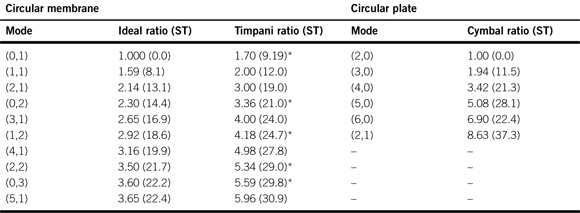
Drums consist of membranes or “drum heads,” which are either made of a synthetic material or animal skin, stretched across a supporting frame which is usually round. A small hand-drum, such as the tabor which is commonly used in early music, consists of a cylindrical ring with the drum head stretched across one end, the other end being open. This construction is also used for the tambourine, which is like a tabor but with small cymbal-like disks, or “jingles,” mounted in pairs on pins in slots around the cylindrical ring. These rattle together when the instrument is mechanically excited, either by striking it with the knuckles or fingertips to set the jingles ringing briefly, or by rubbing a thumb around the head near the edge to set the jingles ringing continuously. Larger drums exist which have a single head stretched over a long cylinder, such as congas and bongos, and these are usually struck with the player’s hands.
The drums found in a drum kit are the bass drum, snare drum and two or more tom-toms of different sizes. These, along with the orchestral bass drum, have two drum heads—one mounted on each side of their cylindrical ring. Bass and snare drums are set up so as to be essentially non-pitched by setting a different tension on each of the drum heads, and therefore spreading the non-harmonic modes produced by the two heads widely in frequency. When they are struck the result is not pitch specific, and therefore they can be used to provide rhythm for music in any key. The snare drum (or “side drum” in marching bands) has a set of metal wires stretched across its lower head (or “snare head”), which vibrate against the snare head when the drum’s upper head or “batter head” is struck. The snares can be dropped from the snare head by means of a lever to allow the drum to be used without the vibrating snare. Tom-toms on the other hand are often tuned so as to provide a more definite sense of pitch by matching more closely the tuning of the upper and lower heads on each drum. They are often used in fills to give rising or, more commonly, falling groups of multiple strikes during a fill.
While the tom–tom can produce a more definite sense of pitch, it is not the clearest that can be achieved from a drum. The main orchestral drum is the kettledrum, and there will usually be between two and five kettle-drums used in today’s orchestras with a single player devoted to playing them. Such a group of kettledrums is referred to as “timpani” (the Oxford Companion to Music notes that “tympani” is a common misspelling of “timpani”); therefore a single kettledrum would be a “timpano.” As the music modulates from one key to another, composers can continue to make use of the timpani in the new key since they can be retuned rapidly.
A kettledrum has a single membrane which is stretched over a metal bowl (or kettle) that is suspended on a supporting frame. Absolute tuning of a kettledrum head is set by means of adjusting screws (usually eight) around its rim, to enable it to be tuned to the appropriate absolute pitch reference. During a performance, its tuning can be changed in semitone steps by means of a lever tensioning system operated by a pedal, which typically enables a pitch variation over five semitones. The head tension varies as the lever is moved from note to note, and, if the kettledrum is struck immediately prior to the lever being moved, a rising (or falling) pitch is heard as a glide or glissando. This is sometimes used for musical effect.
The modes produced when a kettledrum is struck are the same shape as those given in Figure 4.31, but their mode frequencies are different from those of an unmounted head (shown as “ideal” in Table 4.2), because of the effect of the air in the bowl over which the head is stretched and the position at which it is struck. Hall (2001) describes this as follows: “When sections of the head move into and out of the bowl, other sections move in the opposite direction (out of and into the bowl respectively).” These are marked in Figure 4.31 with plus and minus signs. The (0,1) mode is an exception to this, and it is marked with “−/+” since it involves the whole head moving either into or out of the bowl, as it attempts to compress and rarefy the trapped air respectively.
In practice, this mode is damped by means of a vent hole in the bowl which allows air to move out of and into the bowl in response to this mode, thereby absorbing its energy. This vent hole has no such effect on the other modes since they all involve compensating movements by sections of the head as indicated by the equal numbers of plus and minus signs in Figure 4.31. Hall notes that the usual strike position for a kettledrum is half to three quarters of the distance from the center to the rim, and that this is reasonably close to the circular node positions for all modes that have two or three circular nodes: {(0,2), (1,2), (2,2) and (0,3)} in Figure 4.31. These modes will not be greatly excited since they will be unable to realize strong circular nodes due to the strike producing a significant velocity in their circular nodal regions (see Section 4.2.1 on modes not excited when a string is plucked).
In summary, only modes with one circular node (the one they must all have at the rim) except the first mode (0,1) contribute significantly to the sound produced by a kettledrum, bearing in mind that this depends on the strike position being between a half and three quarters of the distance from the drum center to the rim. The presence of the bowl lowers the frequencies of these contributing modes since the head is effectively made more massive due to the presence of the air trapped in the bowl which loads it. The extent of the pitch flattening of the modes is dependent on the shape of the bowl itself, and the aim for the kettledrum maker is to achieve modal frequencies for the modes with one circular mode that are close to being members of the same harmonic series.
Table 4.2 shows the frequency ratios for the lowest 10 modes of an ideal supported membrane (these are the modes shown in Figure 4.31), and those for a kettledrum (adapted from Rossing, 2001). The modes that do not contribute significantly to the overall output from a kettledrum {(0,1), (0,2), (1,2), (2,2) and (0,3)} are indicated with an asterisk. It can be seen that the frequency ratios of the remaining modes are very close to being the second, third, fourth, fifth and sixth harmonics—making the kettledrum an orchestral instrument whose output has a “missing fundamental”—but this does not affect our ability to perceive its pitch as being associated with the missing fundamental as discussed in Section 3.2.1. A kettledrum then will output a strongly pitched note, provided it is struck in a position that tends not to favor those modes marked with an asterisk in Table 4.2.
The player does then have some control over the output spectrum from a kettledrum depending on where it is struck. Note that a strike in the center is not very satisfactory in terms of the resulting sound because almost all of the first 10 modes have nodes in the center, and therefore they will tend not to be excited. Another form of control is from the use of different mallets. Small hard mallets produce a large excitation that is focused over a small area and therefore can excite a number of modes extending to high frequencies, while the excitation from large soft mallets is somewhat muffled, duller and less strong due to it being spread over a larger area, thereby tending to excite more strongly the lower frequency modes. This muffling effect was produced on early kettledrums by placing a cloth over the drum head. The normal orchestral playing effects for timpani are the roll and repeated notes.
The lower part of Figure 4.31 shows the first six modes of a cymbal (Rossing, 2001). It should be noted that unlike the stretched membrane a metal plate is not supported around its outer edge, and therefore the low-frequency modes have no circular nodes. Rossing notes that the modes above the sixth tend to be combinations of more than one individual mode, and are therefore rather difficult to pin down in terms of their modal patterns, but they do tend to have at least one circular node. The mode frequencies do not approximate closely to a harmonic series and therefore no strong pitch is produced by cymbals. Cymbals are struck in a variety of ways, either as a pair of orchestral crash cymbals or as a “hi-hat” in a drum kit or with hard or soft beaters. Crash and hi-hat cymbals excite all modes since all modes have antinodes around the edges of the cymbals. The use of beaters gives the player some control of the output spectrum in the same way that is described for a kettledrum above.
4.5 The Speaking and Singing Voice
The singing voice is probably the most versatile of all musical instruments. Anyone who can speak is capable of singing, but we are not all destined to be opera or pop stars. While considerable mystique surrounds the work of some singing teachers and how they achieve their results, the acoustics of the singing voice is now established as a research topic in its own right. Issues such as the following are being considered:
- the differences between adult male and adult female voices;
- the effects of singing training;
- the development of pitching skills by children;
- “tone deafness;”
- the acoustic nature of different singing styles;
- the effect of different acoustics on choral singing;
- electronic synthesis of the singing voice;
- choral blend in choirs;
- solo voice.
Knowledge of the acoustics of the singing and speaking voice can be helpful to music technologists when they are developing synthetic sounds since humans are remarkably good at vocalizing the sound they desire. In such cases, knowledge of the acoustics of the singing and speaking voice can help in the development of synthesis strategies. This section discusses the human singing voice in terms of the input/system/output model and points to some of the key differences between the speaking and singing voice. The discussion presented in this section is necessarily brief. A number of texts are available which consider the acoustics of the speaking voice (e.g., Fant, 1960; Fry, 1979; Borden and Harris, 1980; Baken, 1987; Baken and Danilof, 1991; Kent and Read, 1992; Howard, 1998; Howard and Angus, 1998), and the acoustics of the singing voice (e.g., Benade, 1976; Sundberg, 1987; Bunch, 1993; Dejonckere et al., 1995; Howard, 1999).
The sound source in singing is the acoustic result of the vocal folds vibrating in the larynx which is sustained by air flowing from the lungs. The sound modifiers in singing are the spaces between the larynx and the lips and nostrils, known as the “vocal tract,” which can be changed in shape and size by moving the “articulators,” for example the jaw, tongue and lips (see Figure 4.32). As we sing or speak, the shape of the vocal tract is continually changing to produce different sounds. The soft palate acts as a valve to shut off and open the nasal cavity (nose) from the airstream.

Figure 4.32 A cross-section of the vocal tract.
Vocal fold vibration in a healthy larynx is a cyclic sequence in which the vocal folds close and open regularly when a note is being sung. Thus the vocal folds of a soprano singing A4 (f0 = 440.0 Hz) will complete this vocal fold closing and opening sequence 440 times a second. Singers have two methods by which they can change the f0 of vocal fold vibration: they alter the stiffness of the folds themselves by changing the tension of the fold muscle tissue, or by altering the vibrating mass by supporting an equal portion of each fold in an immobile position. Adjustments of the physical properties of the folds themselves allow many trained singers to sing over a pitch range of well over two octaves.
The vocal folds vibrate as a result of the Bernoulli effect in much the same way as the lips of a brass player. A consequence of this is that the folds close more rapidly than they open. An acoustic pressure pulse is generated at each instant when the vocal folds snap together, rather like a hand clap. As these closures occur regularly during singing, the acoustic input to the vocal tract consists of a regular series of pressure pulses (see Figure 4.33), the note being sung depending on the number per second. The pressure pulses are shown as negative-going in the figure since the rapid closure of the vocal folds suddenly causes the airflow from the lungs to stop, resulting in a pressure drop immediately above the vocal folds. The time between each pulse is the fundamental period. Benade (1976) notes though that the analogy between the lip vibration of brass players and vocal fold vibration speakers and singers should not be taken too far because the vocal folds can vibrate with little influence being exerted by the presence of the vocal tract, whereas the brass player’s lip vibration is very strongly influenced by the presence of the instrument’s pipe.

Figure 4.33 Idealized waveform (left) and spectrum (right) of acoustic excitation due to normal vocal fold vibration. (Note that T0 indicates the period of the acoustic excitation waveform, and f0 indicates the fundamental frequency.)
Figure 4.34 shows a schematic vocal fold vibration sequence as if viewed from the front associated with an idealized airflow waveform between the vibrating vocal folds. This is referred to as “glottal” airflow since the space between the vocal folds is known as the “glottis.” Three key phases of the vibration cycle are usefully identified: closed phase (vocal folds together), opening phase (vocal folds parting), and closing phase (vocal folds coming together). The opening and closing phases are often referred to as the “open phase” as shown in the figure, because this is the time during which air flows. It should also be noted that airflow is not necessarily zero during the closed phase since there are vocal fold vibration configurations for which the vocal folds do not come together over their whole length (e.g., Sundberg, 1987; Howard, 1998, 1999).

Figure 4.34 Schematic sequence for two vocal fold vibration cycles to illustrate vocal fold vibration sequence as if viewed from the front, and idealized glottal airflow waveform. Vocal fold opening, closing, open and closed phases are indicated.
The nature of vocal fold vibration changes with voice training, whether for oratory, acting or singing. The time for which the vocal folds are in contact in each cycle, known as “larynx closed quotient” or “CQ,” has been investigated as a possible means by which trained adult male (Howard et al., 1990) and female (Howard, 1995) singers can be helped in producing a more efficient acoustic output. Experimental measurements on trained and untrained singers suggest that CQ is higher at all pitches for trained adult males, and that it tends to increase with pitch for trained adult females in a patterned manner.
Howard et al. suggest that the higher CQ provides the potential for a more efficient voice output by three means: (i) the time in each cycle during which there is an acoustic path via the open vocal folds to the lungs, where sound is essentially completely absorbed, is reduced, (ii) longer notes can be sustained since less air is lost via the open vocal folds in each cycle, and (iii) the voice quality is less breathy since less air flows via the open vocal folds in each cycle.
The frequency spectrum of the regular pressure pulses generated by the vibrating vocal folds during speech and singing consists of all harmonics with an amplitude change on average of–12 dB per octave rise in frequency (see the illustration on the right in Figure 4.33). Thus for every doubling in frequency, equivalent to an increase of one octave, the amplitude reduces by 12 dB. The amplitudes of the first, second, fourth and eighth harmonics (which are separated by octaves) in the figure illustrate this effect.
The shape of the acoustic excitation spectrum remains essentially constant while singing, although the amplitude change of – 12 dB per octave is varied for artistic effect and singing style and to aid voice projection by professional singers (e.g., Sundberg, 1987). The spacing between the harmonics will change as different notes are sung; Figure 4.38 shows three input spectra for sung notes an octave apart. Trained singers, particularly those with Western operatic voices, exhibit an effect known as “vibrato” in which their f0 is varied at a rate of approximately 5.5–7.5 Hz with a range of between ± 0.5 and ± 2 semitones (Dejonckere et al., 1995).
4.5.2 Sound Modifiers in Singing
The regular series of pulses from the vibrating vocal folds are modified by the acoustic properties of the vocal tract (see Figure 4.32). In acoustic terms, the vocal tract can be considered as a stopped tube (closed at the larynx, which operates as a flow-controlled reed, and open at the lips) which is approximately 17.5 cm in length for an adult male. When the vowel at the end of announcer is produced, the vocal tract is set to what is referred to as a “neutral” position, in which the articulators are relaxed, and the soft palate (see Figure 4.32) is raised to cut off the nose; the vowel is termed “non-nasalized.” The neutral vocal tract approximates quite closely to a tube of constant diameter throughout its length and therefore the equation governing modal frequencies in a cylindrical stopped pipe can be used to find the vocal tract standing wave mode frequencies for this vowel.
Example 4.3
Calculate the first three mode frequencies of the neutral adult male vocal tract. (Take the velocity of sound in air as 344 ms−1.)
The vocal tract length is 17.5 cm, or 0.175 m.
From Equation 4.9, the fundamental or first mode:
![]()
From Equation 4.10, the higher mode frequencies are:
fstopped(n) = | (2n − 1) fstopped(1) |
where n = | 1, 2, 3, 4, … |
Thus the second mode frequency (n = 2) is: 3 × 491.4 = 1474 Hz and the third mode frequency (n = 3) is: 5 × 491.4 = 2457 Hz.
Example 4.3 gives the frequencies for the neutral vowel, and these are often rounded to 500 Hz, 1500 Hz and 2500 Hz for convenience. When considering the acoustics of speech and singing, the standing wave modes are generally referred to as “formants.” Idealized frequency response curves for a vocal tract set to produce the vowels in the words fast, feed and food are shown in Figure 4.35 and the center frequency of each formant is labeled starting with “F1” or “first formant” for the peak that is lowest in frequency, continuing with “F2” (second formant) and “F3” (third formant) as shown in the figure. The formants are acoustic resonances of the vocal tract itself resulting from the various dimensions of the vocal tract spaces. These are modified during speech and singing by movements of the articulators.

Figure 4.35 Idealized vocal tract response plots for the vowels in the words fast (a), feed (b), and food (c).
When considering the different sounds produced during speech, usually just the first, second and third formants are considered since these are the only formants whose frequencies tend to vary. Six or seven formants can often be identified in the laboratory and the higher formants are thought to contribute to the individual identity of a speaking or singing voice. However, in singing, important contributions to the overall projection of sound are believed to be made by formants higher than the third.
In order to produce different sounds, the shape of the vocal tract is altered by means of the articulators to change its acoustic properties. The perturbation theory principles explored in the context of woodwind reed instruments (see Figure 4.23) can be employed here also (Kent and Read, 1992). Figure 4.36 shows the velocity nodes and antinode positions for the first three formants of the vocal tract during a neutral non-nasalized vowel, which can be confirmed with reference to the upper-right-hand part of Figure 4.23. Following the same line of reasoning as that presented in the context of Figure 4.23, the effect of constrictions (and therefore enlargements) on the first three formants of the vocal tract can be predicted as shown in Figure 4.37. For example, all formants have a volume velocity antinode at the lips, and a lip constriction therefore lowers the frequencies of all formants. (It should be noted that there are two other means of lowering all formant frequencies by means of vocal tract lengthening either by protruding the lip or by lowering the larynx.)

Figure 4.36 Velocity nodes and antinode positions for the first three modes (or formants: F1, F2, F3) of the vocal tract during a neutral non-nasalized vowel.

Figure 4.37 Formant frequency modification with position of vocal tract of constriction.
A commonly referenced set of average formant frequency values for men, women and children for a number of vowels, taken from Peterson and Barney (1952), is shown in Table 4.3. Formant frequency values for these vowels can be predicted with reference to their articulation. For example, the vowel in beat has a constriction towards the front of the tongue in the region of both N2 and N3 (see Figure 4.36), and reference to Figure 4.37 suggests that F1 is lowered in frequency and F2 and F3 are raised from the values one would expect for the neutral vowel. The vowel in part, on the other hand, has a significant constriction in the region of both A2 and A3 (see Figure 4.36) resulting in a raising of F1, and a lowering of both F2 and F3 from their neutral vowel values. The vowel in boot has a constriction at the lips, which are also rounded so as to extend the length of the vocal tract, and thus all formant frequencies are lowered from their neutral vowel values. These changes can be confirmed from Table 4.3.
Table 4.3 Average formant frequencies in Hz for men, women and children for a selection of vowels. (From Peterson and Barney, 1952.)

The input/system/output model for singing consists of the acoustic excitation due to vocal fold vibration (input) and the vocal tract response (system) to give the output. These are usually considered in terms of their spectra, and both the input and system change with time during singing. Figure 4.38 shows the model for the vowel in fast sung on three different notes. This is to allow one of the main effects of singing at different pitches to be illustrated.

Figure 4.38 Singing voice input/system/output model idealized for the vowel in fast sung on three notes an octave apart.
The input in each case is the acoustic spectrum resulting from vocal fold vibration (see Figure 4.33). The output is the result of the response of the vocal tract for the vowel in fast acting on the input vocal fold vibration. The effect of this is to multiply the amplitude of each harmonic of the input by the response of the vocal tract at that frequency. This effectively imparts the formant peaks of the vocal tract response curve onto the harmonics of the input spectrum. In this example, there are three formant peaks shown, and it can be seen that in the cases of the lower two notes the formant structure can be readily seen in the output, but that in the case of the highest note the formant peaks cannot be identified in the output spectrum because the harmonics of the input are too far apart to represent clearly the formant structure.
The representation of the formant structure in the output spectrum is important if the listener is to identify different vowels. Figure 4.38 suggests that somewhere between the G above middle C and the G an octave above, vowel identification will become increasingly difficult. This is readily tested by asking a soprano to sing different vowels on mid and top G, as shown in the figure, and listening to the result. In fact, when singing these higher notes, professional sopranos adopt vocal tract shapes which place the lower formants over individual harmonics of the excitation so that they are transmitted via the vocal tract with the greatest amplitude. In this way, sopranos can produce sounds of high intensity which will project well. This effect is used from approximately the C above middle C where the vocal tract is, in effect, being “tuned in” to each individual note sung, but at the expense of vowel clarity.
This tuning-in effect is not something that tenors need to do since the ratio between the formant frequencies and the f0 of the tenor’s range is higher than that for sopranos. However, all singers who do not use amplification need to project above accompaniment, particularly when this is a full orchestra and the performance is in a large auditorium. The way in which professional opera singers achieve this can be seen with reference to Figure 4.39, which shows idealized spectra for the following:

Figure 4.39 Idealized spectra: (a) a singer speaking the text of an opera aria, (b) the orchestra playing the accompaniment to the aria, (c) the aria being sung with orchestral accompaniments (adapted from Sundberg, 1987).
- a professional opera singer speaking the text of an operatic aria;
- the orchestra playing the accompaniment to the aria; and
- the aria sung by the singer with the orchestral accompaniment.
It should be noted that the amplitude levels cannot be directly compared between (a) and (b) in the figure (i.e. the singer does not speak as loudly as the orchestral accompaniment!) since they have been normalized for comparison.
The idealized spectrum for the text read alone has the same general shape as that for the orchestra playing alone. When the professional singer sings the aria with orchestral accompaniment, it can be seen that this combined response curve has a shape similar to both the speech and orchestral accompaniment at low frequencies, but with an additional broad peak between approximately 2.5 kHz and 4 kHz and centered at about 3 kHz. This peak relates to the acoustic output from the singer when singing but not when speaking, since it is absent for the read text and also in the orchestral accompaniment alone.
This peak has similar characteristics to the formants in the vocal tract response, and for this reason it is known as the “singer’s formant.” The presence of energy in this peak enables the singer to be heard above an accompanying orchestra because it is a section of the frequency spectrum in which the singer’s output prevails. This is what gives the professional singing voice its characteristic “ring,” and it is believed to be the result of lowering the larynx and widening the pharynx (see Figure 4.32) which is adopted by trained Western operatic singers. (The lower plot in Figure 5.5 in Chapter 5 is an analysis of a CD recording of a professional tenor whose singer’s formant is very much in evidence.)
Singing teachers set out to achieve these effects from pupils by suggesting that pupils: “sing on the point of the yawn,” or “sing as if they have swallowed an apple which has stuck in their throat.” Sundberg (1987) discusses the articulatory origin of the singer’s formant as follows: “it shows a strong dependence on the larynx tube,” concluding that: “it is necessary, however, that the pharynx tube be lengthened and that the cross-sectional area in the pharynx at the level of the larynx tube opening be more than six times the area of that opening.”
Professional singing is a complex task which extends the action of the instrument used for speech. It is salutary to note that the prime function of the vocal folds is to act as a valve to protect the lungs, and not to provide the sound source basic to human communication by means of speech and song.
4.5.3 Tuning in a Capella (Unaccompanied) Singing
Experienced singers are able to vary their intonation (sung pitch) to a very fine degree with respect either to the pitch of any accompanying instrument(s) or, if singing a capella (unaccompanied), to the pitches of the other singers. If singing with accompaniment that is being provided by a modern piano or pipe organ, then the tuning system will be equal tempered where all the semitones have a twelfth root of two frequency ratio (see Section 3.4.3).
When singing a capella though, there is no requirement to stick to equal tempered tuning and the possibility exists for singers to make use of the more consonant just intonation where the intervals are maximally consonant (see Section 3.3.3), for example with perfect fifths (frequency ratio 3:2) and just major and minor thirds (frequency ratios 5:4 and 6:5 respectively). Bearing in mind that just intonation cannot be used to tune a 12-note chromatic musical keyboard if the octaves are to remain in the ratio 2:1 (see Section 3.4), there could be musical situations where singing in just intonation causes the overall pitch to drift as a piece modulates through different keys and back to the starting key.
When singers take care with their listening, they will tend away from non-equal tempered tuning towards just tuning (Helmholtz, 1954; Bohrer, 2002). A note sung by one singer has many harmonics whose relative amplitudes depend mainly on the setting of the sound modifiers and therefore the formant frequencies (see Section 4.5.2). When singing a chord, each harmonic of the note produced by one singer will have a nearest neighbor in the set of harmonics produced by another singer and the overall consonance of the result will depend heavily on the tuning accuracy. This is maximized when the fundamental frequencies are in an integer relationship and are harmonics of each other (see Section 3.3.3).
When a capella singing group adopts the non-equal temperament of just tuning, there is the question of whether the group’s pitch remains in-tune or not if the music modulates away from the starting key and back again. In order to test this, some musical exercises were written by Howard (2007a) for a four-part (soprano, alto, tenor, bass or SATB) quartet which involved a four-part block chord movement that visited a large number (compared with the total number) of key chords. An example (Exercise 3) is shown in Figure 4.40 where the first and last chords are spaced by one octave. This exercise was one of a set that has been used to test the hypothesis that an SATB a capella vocal quartet will drift in pitch with key modulation if it tends to non-equal temperament.

Figure 4.40 Tuning exercise to test for pitch drift in a capella singing (from Howard, 2007a).
The f0 of each of the four singers was measured when they sang the set of exercises by means of an electrolaryngograph (Abberton et al., 1989), which monitors vocal fold vibration directly. It makes use of two electrodes that are placed externally on the neck at the level of the larynx. A small high-frequency electrical current flows between the electrodes that is higher when the vocal folds are in contact than when they are apart. Note that acoustic measurements could not be used for f0 measurement in this experiment for four singers since the recordings of each singer would be contaminated with the sound from the other singers.
The predicted pitch drift for just tuning of the chords in the exercise shown in Figure 4.40 is shown in Figure 4.41. It is based on the tuning of the just scale (see Section 3.4.2), and it can be seen that the prediction is for the pitch to drift a semitone flat (rather surprising for an exercise consisting of only 13 chords!).
Figure 4.41 Predicted pitch drift based on just tuning for the exercise shown in. The 13 chords of the exercise are predicted for each part separately and therefore indicated as “note number” on the X axis (adapted from Howard, 2007a).
Figure 4.42 shows the measured results for a quartet where the average f0 for each sung note of each chord has been used (Howard, 2007a). The measured results have a similar trend to that predicted, but with some variation in detail. The singers tend to drift flat more gently than the prediction in the early stages then more rapidly afterwards, with individual singers generally moving together except for the bass whose pitch swings are quite wide from chord to chord. The soprano and to some extent the alto in this quartet seem to be reluctant to allow the pitch to drift any further flat towards the end, almost maintaining it in the position it has reached somewhat against the efforts of the tenor and to some extent the bass to shift it further in line with the prediction. The overall measured pitch change is quite close to the semitone flat shift predicted. The experiment was repeated with this quartet and another quartet sang the exercise twice (Howard, 2007b); the results in each case were similar.

Figure 4.42 Measured pitch drift for a quartet singing the exercise shown in. The 13 chords of the exercise (see Figure 4.40) are analyzed for each part separately and therefore indicated as “note number” on the X axis (adapted from Howard, 2007a).
This experiment confirms that singers do tend towards just tuning and that they maintain this overall tuning even at the expense of the overall pitch of the piece. Thus a dichotomy is presented to choral singers and their conductors in terms of whether to keep the overall pitch in-tune and make some compromise to the tuning of individual chords or whether to allow the overall pitch to drift. Since equal temperament is at the heart of music heard by most people brought up within the Western musical tradition, its compromised intervals in terms of their lack of consonance (all intervals except the octave are out-of-tune) form the basis of how musical intervals are learned.
It is therefore interesting to note the tendency of a capella choral singers towards the more consonant intervals of just intonation which are based on minimum beats, whilst at the same time noting the difficulty of tuning in equal temperament for which there is no readily available physical guide such as the absence of beating. Tuning notes in equal temperament is therefore likely to rely on memories of music from an early age rather than relying on any physical attributes of the relations between the notes themselves.
Howard (2007b) lists a number of basic points in relation to singing a capella in just intonation including:
- Singers do seem able to change their tuning, even subconsciously.
- Singers are not completely “locked” to equal temperament.
- Some consistency in approach has been demonstrated.
- Natural shift is towards just intonation.
- Present one note to start a piece—not an equal tempered chord.
- Have good listening skills.
In addition, he notes some points which tend to work against achieving just tuning including:
- choir practice with a piano or other keyboard tuned in equal temperament;
- listening to recorded and live music in equal temperament;
- working with choral conductors who are unaware of the implications;
- presenting an equal tempered chord to start a piece rather than one note;
- being trained to remain in-tune;
- poor listening skills.
This aspect of a capella singing is one that many choral conductors are unaware of: knowledge of acoustics and psychoacoustics provides the basis for a proper understanding of its underlying causes. Conductors and directors should be aware of the effect and then they can make their own musical judgment in terms of what to do about pitch drift when it arises.
References
Abberton, E.R.M., Howard, D.M., Fourcin, A.J., 1989. Laryngographic assessment of normal voice: a tutorial. Clin. Linguist. Phon. 3, 281–296.
Askenfelt, A. (ed.), 1990. Five Lectures on the Acoustics of the Piano, with compact disc, Publication No. 64. Royal Swedish Academy of Music, Stockholm.
Audsley, G.A., 1965. The Art of Organ-Building 2 Vols. Dover, New York (reprint of 1905 edition, New York: Dodd, Mead and Company).
Baken, R.J., 1987. Clinical Measurement of Speech and Voice. Taylor and Francis, London.
Baken, R.J., Danilof, R.G., 1991. Readings in Clinical Spectrography of Speech. Singular Publishing Group, San Diego.
Benade, A.H., 1976. Fundamentals of Musical Acoustics. Oxford University Press, New York.
Bohrer, J.C.S., 2002. Intonational Strategies in Ensemble Singing [Doctoral thesis]. University of London, London
Borden, G.J., Harris, K.S., 1980. Speech Science Primer. Williams and Wilkins, Baltimore.
Bunch, M., 1993. Dynamics of the Singing Voice. Springer-Verlag, New York.
Campbell, M., Greated, C., 1998. The Musician’s Guide to Acoustics. Oxford University Press, Oxford.
Dejonckere, P.H., Hirano, M., Sundberg, J. (eds), 1995. Vibrato. Singular Publishing Group, San Diego.
Fant, C.G.M., 1960. Acoustic Theory of Speech Production. Mouton, The Hague.
Fletcher, N.H., Rossing, T.D., 1999. The Physics of Musical Instruments, Second edn. Springer-Verlag, New York.
Fry, D.B., 1979. The Physical of Speech. Cambridge University Press, Cambridge
Hall, D.E., 2001. Musical Acoustics: An Introduction, Third edn. Wadsworth Publishing Company, Belmont, CA.
Helmholtz, H., 1954. On the Sensations of Tone, 2nd edn. (1885 translation by A. J. Ellis of the 1877 4th edn.), Dover, New York.
Howard, D.M., 1995. Variation of electrolaryngographically derived closed quotient for trained and untrained adult female singers. J. Voice 9, 163–172.
Howard, D.M., 1998. Practical voice measurement. In: Harris, T., Harris, S., Rubin, J.S., Howard, D.M. (eds), The Voice Clinic Handbook. Whurr Publishing Company, London, 323–382.
Howard, D.M., 1999. The human singing voice. In: Day, P. (Ed.), Killers in the Brain. Oxford University Press, Oxford, pp. 113–134.
Howard, D.M., 2007a. Intonation drift in a capella Soprano, Alto, Tenor, Bass quartet singing with key modulation. J. Voice 21 (3), 300–315.
Howard, D.M., 2007b. Equal or non-equal temperament in a capella SATB singing. Logop. Phoniatr. Vocol. 32 (2), 87–94.
Howard, D.M., Angus, J.A.S., 1998. Introduction to human speech production, human hearing and speech analysis. In: Westall, F.A., Johnson, R.D., Lewis, A.V. (Eds), Speech Technology for Telecommunications. Chapman and Hall, London, pp. 30–72.
Howard, D.M., Lindsey, G.A., Allen, B., 1990. Towards the quantification of vocal efficiency. J. Voice 4, 205–221 (See also errata: (1991). J. Voice, 5, 93–95.)
Hurford, P., 1994. Making Music on the Organ, sixth edn. Oxford University Press, Oxford.
Hutchins, C.M. (ed.), 1975a. Musical Acoustics, Part I: Violin Family Components. Dowden, Hutchinson and Ross Inc, Pennsylvania.
Hutchins, C.M. (ed.), 1975b. Musical Acoustics, Part II: Violin Family Functions. Dowden, Hutchinson and Ross Inc, Pennsylvania.
Hutchins, C.M. (ed.), 1978. The Physics of Music. Reprints from Scientific American, W.H. Freeman and Company, San Francisco.
Kent, R.D., Read, C., 1992. The Acoustic Analysis of Speech. Singular Publishing Group, San Diego.
Martin, D., Ward, D., 1961. Subjective evaluation of musical scale temperament in pianos. J. Acoust. Soc. Am. 33, 582–585.
Nederveen, C.J., 1969. Acoustical Aspects of Woodwind Instruments. Frits Knuf, Amsterdam.
Norman, H., Norman, H.J., 1980. The Organ Today. David and Charles, London.
Peterson, G.E., Barney, H.E., 1952. Control methods used in the study of vowels. J. Acoust. Soc. Am. 24, 175–184.
Rossing, T.D., 2001. The Science of Sound, third edition. Addison-Wesley, New York.
Sumner, W.L., 1975. The Organ, Fifth edn. Macdonald and Company, London.
Sundberg, J., 1987. The Science of the Singing Voice. Illinois University Press, DeKalb.
Sundberg, J., 1989. The Science of Musical Sounds. Academic Press, San Diego.
Taylor, C.A., 1976. Sounds of Music. Butler and Tanner Ltd, London.