Chapter 3: Notes and Harmony

Music of all cultures is based on the use of instruments (including the human voice) which produce notes of different pitches. The particular set of pitches used by any culture may be unique but the psychoacoustic basis on which pitch is perceived is basic to all human listeners. This chapter explores the acoustics of musical notes which are perceived as having a pitch, and the psychoacoustics of pitch perception. It then considers the acoustics and psychoacoustics of different tuning systems that have been used in W estern music.

The representation of musical pitch can be confusing because a number of different notation systems are in use. In this book the system which uses A4 to represent the A above middle C has been adopted. The number changes between the notes B and C, and capital letters are always used for the names of the notes. Thus middle C is C4, the B immediately below it is B3, etc. The bottom note on an 88-note piano keyboard is therefore A0 since it is the fourth A below middle C, and the top note on an 88-note piano keyboard is C8. (This notation system is shown for reference against a keyboard later in the chapter in Figure 3.21.)

Figure 3.21 Fundamental frequency values to four significant figures for eight octaves of notes, four either side of middle C, tuned in equal temperament with a tuning reference of A4 = 440 Hz. (Middle C is marked with a black spot.)

3.1.1 Musical Notes and their Fundamental Frequency

When we listen to a note played on a musical instrument and we perceive it as having a clear unambiguous musical pitch, this is because that instrument produces an acoustic pressure wave which repeats regularly. For example, consider the acoustic pressure waveforms recorded by means of a microphone and shown in Figure 3.1 for A4 played on four orchestral instruments: violin, trumpet, flute and oboe. Notice that in each case, the waveshape repeats regularly, or the waveform is “periodic” (see Chapter 1). Each section that repeats is known as a “cycle” and the time for which each cycle lasts is known as the “fundamental period” or “period” of the waveform. The number of cycles which occur in one second gives the fundamental frequency of the note in hertz (or Hz). The fundamental frequency is often notated as “f₀”, pronounced “F zero” or “F nought”, a practice which will be used throughout the rest of this book. Thus f₀ of any waveform can be found from its period as:

Figure 3.1 Acoustic pressure waveform of A4 (440 Hz) played on a violin, trumpet, flute and oboe. (Note: T indicates one cycle of the waveform.)

and the period from a known f₀ as:

Example 3.1

Find the period of the note G5, and the note an instrument is playing if its measured period is 5.41 ms.

Figure 3.21 gives the f₀ of G5 as 784.0 Hz; therefore its period from Equation 3.2 is:

The f₀ of a note whose measured period is 5.405 ms can be found using Equation 3.1 as:

The note whose f₀ is nearest to 184.8 Hz (from Figure 3.21) is F#3.

For the violin note shown in Figure 3.1, the f₀ equivalent to any cycle can be found by measuring the period of that cycle from the waveform plot from which the f₀ can be calculated. The period is measured from any point in one cycle to the point in the next (or last) cycle where it repeats, for example a positive peak, a negative peak or a point where it crosses the zero amplitude line. The distance marked “T” for the violen in the figure shows where the period could be measured between negative peaks, and this measurement was made in the laboratory to give the period as 2.27 ms. Using Equation 3.1:

This is close to 440 Hz, which is the tuning reference f₀ for A4 (see Figure 3.21). Variation in tuning accuracy, intonation or, for example, vibrato if the note were not played on an open string, will mean that the f₀ measured for any particular individual cycle is not likely to be exactly equivalent to one of the reference f₀ values in Figure 3.21. An average f₀ measurement over a number of individual periods might be taken in practice.

3.1.2 Musical Notes and their Harmonics

Figure 3.1 also shows the acoustic pressure waveforms produced by other instruments when A4 is played. While the periods and therefore the f₀ values of these notes are similar, their waveform shapes are very different. The perceived pitch of each of these notes will be A4 and the distinctive sound of each of these instruments is related to the differences in the detailed shape of their acoustic pressure waveforms, which is how listeners recognize the difference between, for example, a violin, a clarinet and an oboe. This is because acoustic pressure variations produced by a musical instrument that impinge on the listener’s tympanic membrane are responsible for the pattern of vibration set up on the basilar membrane of that ear. It is this pattern of vibration that is then analyzed in terms of the frequency components of which they are comprised (see Chapter 2). If the pattern of vibration on the basilar membrane varies when comparing different sounds, for example from a violin and a clarinet, then the sounds are perceived as having a different “timbre” (see Chapter 5) whether or not they have the same pitch.

Every instrument therefore has an underlying set of partials in its spectrum (see Chapter 1) from which we are able to recognize it from other instruments. These can be thought of as the frequency component “recipe” underlying the particular sound of that instrument. Figure 3.1 shows the acoustic pressure waveform for different notes played on four orchestral instruments and Figure 3.2 shows the amplitude–frequency spectrum for each. Notice that the shape of the waveform for each of the notes is different and so is the recipe of frequency components. Each of these notes would be perceived as being the note A4 but as having different timbres. The frequency components of notes produced by any pitched instrument, such as a violin, oboe, clarinet, trumpet, etc., are harmonics, or integer (1, 2, 3, 4, 5, etc.) multiples of f₀ (see Chapter 1). Thus the only possible frequency components for the acoustic pressure waveform of the violin note shown in Figure 3.1 whose f₀ is 440.5 Hz are: 440.5 Hz (1 × 440.5 Hz); 881.0 Hz (2 × 440.5 Hz); 1321.5 Hz (3 × 440.5 Hz); 1762 Hz (4 × 440.5 Hz); 2202.5 Hz (5 × 440.5 Hz); etc. Figure 3.2 shows that these are the only frequencies at which peaks appear in each spectrum (see Chapter 1). These harmonics are generally referred to by their “harmonic number,” which is the integer by which f₀ is multiplied to calculate the frequency of the particular component of interest.

Figure 3.2 Spectra of waveforms shown in Figure 3.1 for A4 (f₀ = 440Hz) played on a violin, trumpet, flute and oboe.

An earlier term still used by many authors for referring to the components of a periodic waveform is “overtones.” The first overtone refers to the first frequency component that is “over” or above f₀, which is the second harmonic. The second overtone is the third harmonic, and so on. Table 3.1 summarizes the relationship between f₀, overtones and harmonics for integer multipliers from 1 to 10.

Table 3.1 The relationship between overtone series, harmonic series and fundamental frequency for the first 10 components of a period waveform

Example 3.2

Find the fourth harmonic of a note whose f₀ is 101 Hz, and the sixth overtone of a note whose f₀ is 120 Hz.

The fourth harmonic has a frequency that is (4 f₀), which is (4 × 101) Hz = 404 Hz.

The sixth overtone has a frequency that is (7 f₀), which is (7 × 120) Hz = 840 Hz.

There is no theoretical upper limit to the number of harmonics which could be present in the output from any particular instrument, although for many instruments there are acoustic limits imposed by the structure of the instrument itself. An upper limit can be set though, in terms of the number of harmonics which could be present based on the upper frequency limit of the hearing system, for which a practical limit might be 16 000 Hz (see Chapter 2). Thus an instrument playing the A above middle C, which has an f₀ of 440 Hz, could theoretically contain 36 (= 16 000/440) harmonics within the human hearing range. If this instrument played a note an octave higher, f₀ is doubled to 880 Hz, and the output could now theoretically contain 18 (= 16 000/880) harmonics. This is an increasingly important consideration since although there is often an upper frequency limit to an acoustic instrument which is well within the practical upper frequency range of human hearing, it is quite possible with electronic synthesizers to produce sounds with harmonics which extend beyond this upper frequency limit.

3.1.3 Musical Intervals between Harmonics

Acoustically, a note perceived to have a distinct pitch contains frequency components that are integer multiples of f₀ usually known as “harmonics.” Each harmonic is a sine wave and since the hearing system analyzes sounds in terms of their frequency components it turns out to be highly instructive, in terms of understanding how to analyze and synthesize periodic sounds, as well as being central to the development of Western musical harmony, to consider the musical relationship between the individual harmonics themselves. The frequency ratios of the harmonic series are known (see Table 3.1) and their equivalent musical intervals, frequency ratios and staff notation in the key of C are shown in Figure 3.3 for the first 10 harmonics. The musical intervals (apart from the octave) are only approximated on a modern keyboard due to the tuning system used, as discussed in Section 3.3.

Figure 3.3 Frequency ratios and common musical intervals between the first 10 harmonics of the natural harmonic series of C3 against a musical stave and keyboard.

The musical intervals of adjacent harmonics in the natural harmonic series starting with the fundamental or first harmonic, illustrated on a musical stave and as notes on a keyboard in Figure 3.3, are: octave (2:1), perfect fifth (3:2), perfect fourth (4:3), major third (5:4), minor third (6:5), flat minor third (7:6), sharp major second (8:7), a major whole tone (9:8), and a minor whole tone (10:9). The frequency ratios for intervals between non-adjacent harmonics in the series can also be inferred from the figure. For example, the musical interval between the fourth harmonic and the fundamental is two octaves and the frequency ratio is 4:1, equivalent to a doubling for each octave. Similarly the frequency ratio for three octaves is 8:1, and for a twelfth (octave and a fifth) is 3:1.

Ratios for other commonly used musical intervals can be found from the ones just mentioned (musical intervals which occur within an octave are illustrated in Figure 3.15). To demonstrate this for a known result, the frequency ratio for a perfect fourth (4:3) can be found from that for a perfect fifth (3:2) since together they make one octave (2:1): C to G (perfect fifth) and G to C (perfect fourth). The perfect fifth has a frequency ratio 3:2 and the octave a ratio of 2:1. Bearing in mind that musical intervals are ratios in terms of their frequency relationships and that any mathematical manipulation must therefore be carried out by means of division and multiplication, the ratio for a perfect fourth is that for an octave divided by that for a perfect fifth, or up one octave and down a fifth:

Figure 3.15 All two-note musical intervals occurring up to an octave related to C4.

Two other common intervals are the major sixth and minor sixth, and their frequency ratios can be found from those for the minor third and major third respectively since in each case they combine to make one octave.

Example 3.3

Find the frequency ratio for a major and a minor sixth given the frequency ratios for an octave (2:1), a minor third (6:5) and a major third (5:4).

A major sixth and a minor third together span one octave. Therefore:

A minor sixth and a major third together span one octave. Therefore:

These ratios can also be inferred from knowledge of the musical intervals and the harmonic series. Figure 3.3 shows that the major sixth is the interval between the fifth and third harmonics—in this example these are G4 and E5—and therefore their frequency ratio is 5:3. Similarly the interval of a minor sixth is the interval between the fifth and eighth harmonics, in this case E5 and C6; therefore the frequency ratio for the minor sixth is 8:5. Knowledge of the notes of the harmonic series is both musically and acoustically useful and is something that all brass players and organists who understand mutation stops (see Section 5.4) are particularly aware of.

Figure 3.4 shows the positions of the first 10 harmonics of A3 (f₀ = 220.0Hz), plotted on a linear and a logarithmic axis. Notice that the distance between the harmonics is equal on the linear plot and therefore the harmonics becomes progressively closer together as frequency increases on the logarithmic axis. While the logarithmic plot might appear more complex than the linear plot at first glance in terms of the distribution of the harmonics themselves, particularly given that nature often appears to make use of the most efficient process, notice that when different notes are plotted, in this case E4 (f₀ = 329.6 Hz) and A4 (f₀ = 440.0 Hz), the patterning of the harmonics remains constant on the logarithmic scale but they are spaced differently on the linear scale. This is an important aspect of timbre perception which will be explored further in Chapter 5.

Figure 3.4 The positions of the first 10 harmonics of A3 (f₀ = 220Hz), E4 (f₀ = 330Hz), and A4(f₀ = 440 Hz) on linear (upper) and logarithmic (lower) axes.

Bearing in mind that the hearing system carries out a frequency analysis due to the place analysis which is based on a logarithmic distribution of position with frequency on the basilar membrane, the logarithmic plot most closely represents the perceptual weighting given to the harmonics of a note played on a pitched instrument.

The use of a logarithmic representation of frequency in perception has the effect of giving equal weight to the frequencies of components analyzed by the hearing system that are in the same ratio. Figure 3.5 shows a number of musical intervals plotted on a logarithmic scale and in each case they continue up to around the upper useful frequency limit of the hearing system. In this case they are all related to A1 (f₀ = 55 Hz) for convenience. Such a plot could be produced relative to an f₀ value for any note and it is important to notice that the intervals themselves would remain a constant distance on a given logarithmic scale. This can be readily verified with a ruler, for example by measuring the distance equivalent to an octave from 100 Hz (between 100 and 200 Hz, 200 and 400 Hz, 400 and 800 Hz, etc.) on the x axis of Figure 3.5 and comparing this with the distance between any of the points on the octave plot. The distance anywhere on a given logarithmic axis that is equivalent to a particular ratio such as 2:1, 3:2, 4:3, etc. will be the same no matter where on the axis it is measured.

Figure 3.5 Octaves, perfect fifths, perfect fourths, major sixths and minor thirds plotted on a logarithmic scale relative to A1 (f₀ = 55 Hz).

A musical interval ruler could be made which is calibrated in musical intervals to enable the frequencies of notes separated by particular intervals to be readily found on a logarithmic axis. Such a calibration must, however, be carried out with respect to the length of the ratios of interest: octave (2:1), perfect fifth (3:2), major sixth (5:3), etc. If the distance equivalent to a perfect fifth is added to the distance equivalent to a perfect fourth, the distance for one octave will be obtained since a fifth plus a fourth equals one octave. Similarly, if the distance equivalent to a major sixth is added to that for a minor third, the distance for one octave will again be obtained since a major sixth plus a minor third equals one octave (see Example 3.3).

A doubling (or halving) of a value anywhere on a logarithmic frequency scale is equivalent perceptually to a raising (or lowering) by a musical interval of one octave, and multiplying by (or by ) is equivalent perceptually to a raising (or lowering) by a musical interval of a perfect fifth, and so on. We perceive a given musical interval (octave, perfect fifth, perfect fourth, major third, etc.) as being similar no matter where in the frequency range it occurs. For example, a two-note chord a major sixth apart whether played on two double basses or two flutes gives a similar perception of the musical interval. In this way, the logarithmic nature of the place analysis mechanism provides a basis for understanding the nature of our perception of musical intervals and of musical pitch.

By way of contrast and to complete the story, sounds which have no definite musical pitch (but a pitch, nevertheless—see below) associated with them, such as the “ss” in sea (Figure 3.9 later in the chapter), have an acoustic pressure waveform that does not repeat regularly, and is often random in its variation with time and is therefore not periodic. Such a waveform is referred to as being “aperiodic” (see Chapter 1). The spectrum of such sounds contains frequency components that are not related as integer multiples of some frequency, and there are no harmonic components. The spectrum will often contain all frequencies, in which case it is known as a “continuous” spectrum. An example of an acoustic pressure waveform and spectrum for a non-periodic sound is illustrated in Figure 3.6 for a snare drum being brushed.

Figure 3.9 Waveforms and spectra for “ss” as in sea and “sh” as in shoe.

Figure 3.6 Acoustic pressure waveform (upper) and spectrum (lower) for a snare drum being brushed

3.2 Hearing Pitch

The perception of pitch is basic to the hearing of tonal music. Familiarity with current theories of pitch perception as well as other aspects of psychoacoustics enables a well founded understanding of musically important matters such as tuning, intonation, perfect pitch, vibrato, electronic synthesis of new sounds, and pitch paradoxes (see Chapter 5).

Pitch relates to the perceived position of a sound on a scale from low to high and its formal definition by the American National Standards Institute (1960) is couched in these terms as: “pitch is that attribute of auditory sensation in terms of which sounds may be ordered on a scale extending from low to high.” The measurement of pitch is therefore “subjective” because it requires a human listener (the “subject”) to make a perceptual judgment. This is in contrast to the measurement in the laboratory of, for example, the fundamental frequency (f₀) of a note, which is an “objective” measurement.

In general, sounds which have a periodic acoustic pressure variation with time are perceived as having a pitch associated with them, and sounds whose acoustic pressure waveform is non-periodic are perceived as having no pitch. The relationship between the waveforms and spectra of pitched and non-pitched sounds is summarized in Table 3.2 and examples of each have been discussed in relation to Figures 3.2 and 3.6. The terms “time domain” and “frequency domain” are widely used when considering time (waveform) and frequency (spectral) representations of signals.

Table 3.2 The nature of the waveforms and spectra for pitched and non-pitched sounds

	Pitched	Non-pitched
Waveform	Periodic	Non-periodic
(time domain)	regular repetitions	no regular repetitions
Spectrum	Line	Continuous
(frequency domain)	harmonic components	no harmonic components

The pitch of a note varies as its f₀ is changed: the greater the f₀ the higher the pitch and vice versa. Although the measurement of pitch and f₀ are subjective and objective and measured on a scale of high/low and Hz respectively, a measurement of pitch can be given in Hz. This is achieved by asking a listener to compare the sound of interest by switching between it and a sine wave with a variable frequency. The listener would adjust the frequency of the sine wave until the pitches of the two sounds are perceived as being equal, at which point the pitch of the sound of interest is equal to the frequency of the sine wave in Hz.

Two basic theories of pitch perception have been proposed to explain how the human hearing system is able to locate and track changes in the f₀ of an input sound: the “place” theory and the “temporal” theory. These are described below along with their limitations in terms of explaining observed pitch perception effects.

3.2.1 Place Theory of Pitch Perception

The place theory of pitch perception relates directly to the frequency analysis carried out by the basilar membrane in which different frequency components of the input sound stimulate different positions, or places, on the membrane. Neural firing of the hair cells occurs at each of these places, indicating to higher centers of neural processing and the brain which frequency components are present in the input sound. For sounds in which all the harmonics are present, the following are possibilities for finding the value of f₀ based on a place analysis of the components of the input sound and allowing for the possibility of some “higher processing” of the component frequencies at higher centers of neural processing and/or the brain.

Method 1: Locate the f₀ component itself.
Method 2: Find the minimum frequency difference between adjacent harmonics. The frequency difference between the (n + 1)th and the (n)th harmonic, which are adjacent by definition if all harmonics are present, is:

Method 3: Find the highest common factor (the highest number that will divide into all the frequencies present giving an integer result) of the components present. Table 3.3 illustrates this for a sound consisting of the first 10 harmonics whose f₀ is 100 Hz, by dividing each frequency by integers, in this case up to 10, and looking for the largest number in the results which exists for every frequency. The frequencies of the harmonics are given in the left-hand column (the result of a place analysis), and each of the other columns shows the result of dividing the frequency of each component by integers (m = 2 to 10). The highest common factor is the highest value appearing in all rows of the table, including the frequencies of the components themselves (f₀ ÷ 1) or (m = 1), and is 100 Hz, which would be perceived as the pitch.
In addition, it is of interest to notice that every value which appears in the row relating to the f₀, in this case 100 Hz, will appear in each of the other rows if the table were extended far enough to the right. This is the case because by definition, 100 divides into each harmonic frequency to give an integer result (n) and all values appearing in the 100 Hz row are found by integer (m) division of 100 Hz; therefore all values in the 100 Hz row can be gained by division of harmonic frequencies by (m × n), which must itself be an integer. These are f₀ values (50 Hz, 33 Hz, 25 Hz, 20 Hz, etc.) whose harmonic series also contain all the given components, and they are known as “sub-harmonics.” This is why it is the highest common factor which is used.

Table 3.3 Processing method to find the highest common factor of the frequencies of the first 10 harmonics of a sound whose f₀ = 100 Hz (calculations to four significant figures)

One of the earliest versions of the place theory suggests that the pitch of a sound corresponds to the place stimulated by the lowest frequency component in the sound which is f₀ (Method 1 above). The assumption underlying this is that f₀ is always present in sounds and the theory was encapsulated by Ohm in his second or “acoustical” law¹: “a pitch corresponding to a certain frequency can only be heard if the acoustic wave contains power at that frequency.”

This theory came under close scrutiny when it became possible to carry out experiments in which sounds could be synthesized with known spectra. Schouten (1940) demonstrated that the pitch of a pulse wave remained the same when the fundamental component was removed, thus demonstrating: (i) that f₀ did not have to be present for pitch perception, and (ii) that the lowest component present is not the basis for pitch perception because the pitch does not jump up by one octave (since the second harmonic is now the lowest component after f₀ has been removed). This experiment has become known as “the phenomenon of the missing fundamental,” and suggests that Method 1 cannot account for human pitch perception.

Method 2 seems to provide an attractive possibility since the place theory gives the positions of the harmonics, whether or not f₀ is present, and it should provide a basis for pitch perception provided some adjacent harmonics are present. For most musical sounds, adjacent harmonics are indeed present. However, researchers are always looking for ways of testing psychoacoustic theories, in this case pitch perception, by creating sounds for which the perceived pitch cannot be explained by current theories. Such sounds are often generated electronically to provide accurate control over their frequency components and temporal development.

Figure 3.7 shows an idealized spectrum of a sound which contains just odd harmonics (1 f₀, 3 f₀, 5 f₀, …) and shows that measurement of the frequency distance between adjacent harmonics would give f₀, 2 f₀, 2 f₀, 2 f₀, etc. The minimum spacing between the harmonics is f₀, which gives a possible basis for pitch perception. However, if the f₀ component were removed (imagine removing the dotted f₀ component in Figure 3.7), the perceived pitch would not change. Now, however, the spacings between adjacent harmonics is 3 f₀, 2 f₀, 2 f₀, 2 f₀, etc. and the minimum spacing is 2 f₀, but the pitch does not jump up by an octave.

Figure 3.7 An idealized spectrum for a sound with odd harmonics only to show the spacing between adjacent harmonics when the fundamental frequency component (shown dashed) is present or absent.

The third method will give an appropriate f₀ for: (i) sounds with missing f₀ components (see Table 3.3 and ignore the f₀ row), (ii) sounds with odd harmonic components only (see Table 3.3 and ignore the rows for the even har monics), and (iii) sounds with odd harmonic components only with a missing f₀ component (see Table 3.3 and ignore the rows for f₀ and the even harmonics). In each case, the highest common factor of the components is f₀. This method also provides a basis for understanding how a pitch is perceived for non-harmonic sounds, such as bells or chime bars, whose components are not exact harmonics (integer multipliers) of the resulting f₀.

As an example of such a non-harmonic sound, Schouten in one of his later experiments produced sounds whose component frequencies were 1040 Hz, 1240 Hz, and 1440 Hz and found that the perceived pitch was approximately 207 Hz (consider track 4C on the accompanying CD). The f₀ for these components, based on the minimum spacing between the components (Method 2), is 200 Hz. Table 3.4 shows the result of applying Method 3 (searching for the highest common factor of these three components) up to an integer divisor of 10. Schouten’s proposal can be interpreted in terms of this table by looking for the closest set of values in the table that would be consistent with the three components being true harmonics and taking their average to give an estimate of f₀. In this case, taking 1040 Hz as the fifth “harmonic,” 1240 Hz as the sixth “harmonic” and 1440 Hz as the seventh “harmonic” gives 208 Hz, 207 Hz and 206 Hz respectively. The average of these values is 207 Hz, and Schouten referred to the pitch perceived in such a situation as the “residue pitch” or “pitch of the residue.” It is also sometimes referred to as “virtual pitch.”

Table 3.4 Illustration of how finding the highest common factor of the frequencies of the three components—1040 Hz, 1240 Hz and 1440 Hz—gives a basis for explaining a perceived pitch of approximately 207 Hz (calculations to four significant figures)

By way of a coda to this discussion, it is interesting to note that these components 1040 Hz, 1240 Hz and 1440 Hz do, in fact, have a true f₀ of 40 Hz of which they are the 26th, 31st and 36th harmonics, which would appear if the table were continued well over to the right. However, the auditory system appears to find an f₀ for which the components present are adjacent harmonics.

3.2.2 Problems with the Place Theory

The place theory provides a basis for understanding how f₀ could be found from a frequency analysis of components. However, there are a number of problems with the place theory because it does not explain:

the fine degree of accuracy observed in human pitch perception;
pitch perception of sounds whose frequency components are not resolved by the place mechanism;
the pitch perceived for some sounds which have continuous (non-harmonic) spectra; or
pitch perception for sounds with an f₀ less than 50 Hz.

Each will be considered in turn.

Psychoacoustically, the ability to discriminate between sounds that are nearly the same except for a change in one aspect (f₀, intensity, duration, etc.) is measured as a “difference limen” (DL), or “just noticeable difference” (JND). JND is preferred in this book. The JND for human pitch perception is shown graphically in Figure 3.8 along with the critical bandwidth curve. This JND graph is based on an experiment by Zwicker et al. (1957) in which sinusoidal stimuli were used (fixed waveshape) and the sound intensity level and sound duration remained constant. It turns out that the JND is approximately one thirtieth of the critical bandwidth across the hearing range. Musically, this is equivalent to approximately one twelfth of a semitone. Thus the JND in pitch is much smaller than the resolution of the analysis filters (critical bandwidth).

Figure 3.8 Just noticeable difference (JND) for pitch perception and the equivalent rectangular bandwidth.

The place mechanism will resolve a given harmonic of an input sound provided that the critical bandwidth of the filter concerned is sufficiently narrow to exclude adjacent harmonics. It turns out that, no matter what the f₀ of the sound is, only the first five to seven harmonics are resolved by the place analysis mechanism. This can be illustrated with an example as follows with reference to Table 3.5.

Table 3.5 Illustration of resolution of place mechanism for an input consisting of the first 10 harmonics and an f₀ of 110 Hz (calculations to four significant figures). Key: CB = critical bandwidth, CF = center frequency

Consider a sound consisting of all harmonics (f₀, 2 f₀, 3 f₀, 4 f₀, 5 f₀, etc.) whose f₀ is 110 Hz. The frequencies of the first 10 harmonics are given in the left-hand column of the table. The next column shows the critical bandwidth of a filter centered on each of these harmonics by calculation using Equation 2.6. The critical bandwidth increases with filter center frequency (see Figure 3.8), and the frequency analysis action of the basilar membrane is equivalent to a bank of filters. Harmonics will cease to be resolved by the place mechanism when the critical bandwidth exceeds the frequency spacing between adjacent harmonics, which is f₀ when all adjacent harmonics are present.

In the table, it can be seen that the critical bandwidth is greater than f₀ for the filter centered at 770 Hz (the seventh harmonic), but this filter will resolve the seventh harmonic since it is centered over it and its bandwidth extends half above and half below 770 Hz. In order to establish when harmonics are not resolved, consider the filters centered midway between adjacent harmonic positions (their center frequencies and critical bandwidths are shown in Table 3.5).

The filter centered between the seventh and eighth harmonics has a critical bandwidth of 113.7 Hz which exceeds f₀ (110 Hz in this example) and therefore the seventh and eighth harmonics will not be resolved by this filter. Due to the continuous nature of the wave traveling along the basilar membrane, no harmonics will be resolved in this example above the sixth, since there will be areas on the membrane responding to at least adjacent pairs of harmonics everywhere above the place where the sixth harmonic stimulates it. Appendix 2 shows a method for finding the filter center frequency whose critical bandwidth is equal to a given f₀ by solving Equation 2.6 mathematically.

Example 3.4

Confirm the result illustrated in Table 3.5 that the sixth harmonic will be resolved but the seventh harmonic will not be resolved for an f₀ of 110 Hz.

Using Equation A1.2 in Appendix 1:

Find the center frequency (f_c) for which the critical bandwidth (ERB) equals 110.0 Hz by substituting 110 Hz for ERB. (Bear in mind that the center frequency is in kHz in this equation.)

The center frequency of the filter whose critical bandwidth is 110.0 Hz is 790 Hz. All filters above 790 Hz will have bandwidths that are greater than its bandwidth of 110 Hz, because we know that the critical bandwidth increases with center frequency (see Figure 3.8). As it lies below the center frequency of the filter midway between the seventh (770 Hz) and eighth (880 Hz) harmonics, those harmonics will not be resolved, since the filter that does lie between them will have a bandwidth that is greater than 110 Hz. Therefore harmonics up to the sixth will be resolved and harmonics from the seventh upwards will not be resolved.

Observation of the relationship between the critical bandwidth and center frequency plotted in Figure 3.8 allows the general conclusion that no harmonic above about the fifth to seventh is resolved for any f₀ to be approximately validated as follows. The center frequency for which the critical band exceeds the f₀ of the sound of interest is found from the graph and no harmonic above this center frequency will be resolved. To find the center frequency, plot a horizontal line for the f₀ of interest on the y axis, and find the frequency on the x axis where the line intersects the critical band curve. Only harmonics below this frequency will be resolved and those above will not. It is worth trying this exercise for a few f₀ values to reinforce the general conclusion about resolution of harmonics, since this is vital to the understanding of other aspects of psychoacoustics as well as pitch perception.

There are sounds which have non-harmonic spectra for which a pitch is perceived; these are exceptions to the second part of the general statement given earlier that “sounds whose acoustic pressure waveform is non-periodic are perceived as having no pitch.” For example, listen to examples of the “ss” in sea and the “sh” in shell (produce these yourself or ask someone else to) in terms of which one has the higher pitch. Most listeners will readily respond that “ss” has a higher pitch than “sh.” The spectrum of both sounds is continuous and an example for each is shown in Figure 3.9. Notice that the energy is biased more towards lower frequencies for the “sh” with a peak around 2.5 kHz, compared with the “ss” where the energy has a peak at about 5 kHz.

This “center of gravity” of the spectral energy of a sound is thought to convey a sense of higher or lower pitch for such sounds which are noise based, but the pitch sensation is far weaker than for that perceived for periodic sounds. This pitch phenomenon is, however, important in music when considering the perception of the non-periodic sounds produced, for example, by some groups of instruments in the percussion section (consider track 5 on the accompanying CD), but the majority of instruments on which notes are played in musical performances produce periodic acoustic pressure variations.

The final identified problem is that the pitch perceived for sounds with components only below 50 Hz cannot be explained by the place theory, because the pattern of vibration on the basilar membrane does not appear to change in that region. Sounds of this type are rather unusual, but not impossible to create by electronic synthesis. Since the typical lowest audible frequency for humans is 20 Hz, a sound with an f₀ of 20 Hz would have harmonics at 40 Hz, 60 Hz, etc., and only the first two fall within this region where no change is observed in basilar membrane response. Harmonics falling above 50 Hz will be analyzed by the place mechanism in the usual manner. Sinusoids in the 20–50 Hz range are perceived as having different pitches and the place mechanism cannot explain this.

These are some of the key problems which the place mechanism cannot explain, and attention will now be drawn to the temporal theory of pitch perception which was developed to explain some of these problems with the place theory.

3.2.3 Temporal Theory of Pitch Perception

The temporal theory of pitch perception is based on the fact that the waveform of a sound with a strong musical pitch repeats or is periodic (see Table 3.2). An example is shown in Figure 3.1 for A4 played on four instruments. The f₀ for a periodic sound can be found from a measurement of the period of a cycle of the waveform using Equation 3.1.

The temporal theory of pitch perception relies on the timing of neural firings generated in the organ of Corti (see Figure 2.3) which occur in response to vibrations of the basilar membrane. The place theory is based on the fact that the basilar membrane is stimulated at different places along its length according to the frequency components in the input sound. The key to the temporal theory is the detailed nature of the actual waveform exciting the different places along the length of the basilar membrane. This can be modeled using a bank of electronic band-pass filters whose center frequencies and bandwidths vary according to the critical bandwidth of the human hearing system as illustrated, for example, in Figure 3.8.

Figure 3.10 shows the output waveforms from such a bank of electronic filters, implemented using transputers by Howard et al. (1995), with critical bandwidths based on the ERB equation (Equation 2.6) for C4 played on a violin. The nominal f₀ for C4 is 261.6 Hz (see Figure 3.21 later in the chapter). The output waveform from the filter with a center frequency just above 200 Hz, the lowest center frequency represented in the figure, is a sine wave at f₀. This is because the f₀ component is resolved by the analyzing filter, and an individual harmonic of a complex periodic waveform is a sine wave (see Chapter 1).

Figure 3.10 Output from a transputer-based model of human hearing to illustrate the nature of basilar membrane vibration at different places along its length for C4 played on a violin.

The place theory suggests (see calculation associated with Table 3.5) that the first six harmonics will be resolved by the basilar membrane. It can be seen in the example note shown in Figure 3.10 that the second (around 520 Hz), third (around 780 Hz), fourth (around 1040 Hz) and fifth (around 1300 Hz) harmonics are resolved and their waveforms are sinusoidal. Some amplitude variation is apparent on these sine waves, particularly on the fourth and fifth, indicating the dynamic nature of the acoustic pressure output from a musical instrument. The sixth harmonic (around 1560 Hz) has greater amplitude variation, but the individual cycles are clear.

Output waveforms for filter center frequencies above the sixth harmonic in this example are not sinusoidal because these harmonics are not resolved individually. At least two harmonics are combined in the outputs from filters which are not sinusoidal in Figure 3.10. When two components close in frequency are combined, they produce a “beat” waveform whose amplitude rises and falls regularly if the components are harmonics of some fundamental. The period of the beat is equal to the difference between the frequencies of the two components. Therefore if the components are adjacent harmonics, then the beat frequency is equal to their f₀ and the period of the beat waveform is (1/f₀). This can be observed in the figure by comparing the beat period for filter outputs above 1.5 kHz with the period of the output sinewave at f₀. Thus the period of output waveforms for filters with center frequencies higher than the sixth harmonic will be at (1/f₀) for an input consisting of adjacent harmonics.

The periods of all the output waveforms which stimulate the neural firing in the organ of Corti form the basis of the temporal theory of pitch perception. There are nerve fibers available to fire at all places along the basilar membrane, and they do so in such a manner that a given nerve fiber may only fire at one phase or instant in each cycle of the stimulating waveform, a process known as “phase locking.” Although the nerve firing is phase locked to one instant in each cycle of the stimulating waveform, it has been observed that no single nerve fiber is able to fire continuously at frequencies above approximately 300 Hz. It turns out that the nerve does not necessarily fire in every cycle and that the cycle in which it fires tends to be random, which according to Pickles (1982) may be “perhaps as little as once every hundred cycles on average.”

However, due to phase locking, the time between firings for any particular nerve will always be an integer (1, 2, 3, 4, …) multiple of periods of the stimulating waveform and there are a number of nerves involved at each place. A “volley firing” principle has also been suggested by Wever (1949) in which groups of nerves work together, each firing in different cycles to enable frequencies higher than 300 Hz to be coded. A full discussion of this area is beyond the scope of this book, and the interested reader is encouraged to consult, for example, Pickles (1982), Moore (1982, 1986) and Roederer (1975). What follows relies on the principle of phase locking.

The minimum time between firings (1 period of the stimulating waveform) at different places along the basilar membrane can be inferred from Figure 3.10 for the violin playing C4, since it will be equivalent to the period of the output waveform from the analysis filter. For places which respond to frequencies below about the sixth harmonic, the minimum time between firings is at the period of the harmonic itself, and, for places above, the minimum time between firings is the period of the input waveform itself (i.e., 1/f₀).

The possible instants of nerve firing are illustrated in Figure 3.11. This figure enables the benefit to be illustrated that results from the fact that nerves fire phase locked to the stimulating waveform but not necessarily during every cycle. The figure shows an idealized unrolled basilar membrane with the places corresponding to where maximum stimulation would occur for input components at multiples of f₀ up to the sixteenth harmonic, for any f₀ of input sound. The assumption on which the figure is based is that harmonics up to and including the seventh are analyzed separately. The main part of the figure shows the possible instants where nerves could fire based on phase locking and the fact that nerves may not fire every cycle; the lengths of the vertical lines illustrate the proportion of firings which might occur at that position, on the basis that more firings are likely with reduced times between them. These approximate to the idea of a histogram of firings being built up, sometimes referred to as an “inter-spike interval” histogram, where a “spike” is a single nerve firing.

Figure 3.11 The possible instants for nerve firing across the places on the basilar membrane for the first 16 harmonics of an input sound.

Thus at the place on the basilar membrane stimulated by the f₀ component, possible times between nerve firing are: (1/f₀), (2/f₀) and (3/f₀) in this figure as shown, with fewer firings at the higher intervals. For the place stimulated by the second harmonic, possible firing times are: [1/(2 f₀)], [2/(2 f₀)] or (1/f₀), [3/(2 f₀)], [4/(2 f₀)] or (2/f₀), and so on. This is the case for each place stimulated by a harmonic of f₀ up to the seventh. For places corresponding to higher frequencies than (7 f₀), the stimulating waveform is beat-like and its fundamental period is (1/f₀), and therefore the possible firing times are: (1/f₀), (2/f₀) and (3/f₀) in this figure as shown.

Visually it can be seen in Figure 3.11 that if the entries in all these inter-spike interval histograms were added together vertically (i.e., for each firing time interval), then the maximum entry would occur for the period of f₀. This is reinforced when it is remembered that all places higher than those shown in the figure would exhibit outputs similar to those shown above the eighth harmonic. Notice how all the places where harmonics are resolved have an entry in their histograms at the fundamental period as a direct result of the fact that nerves may not fire in every cycle. This is the basis on which the temporal theory of pitch perception is thought to function.

3.2.4 Problems with the Temporal Theory

The temporal theory gives a basis for understanding how the fundamental period could be found from an analysis of the nerve firing times from all places across the basilar membrane. However, not all observed pitch perception abilities can be explained by the temporal theory alone, the most important being the pitch perceived for sounds whose f₀ is greater than 5 kHz. This cannot be explained by the temporal theory because phase locking breaks down above 5 kHz. Any ability to perceive the pitches of sounds with f₀ greater than 5 kHz is therefore thought to be due to the place theory alone.

Given that the upper frequency limit of human hearing is at best 20 kHz for youngsters, with a more practical upper limit being 16 kHz for those over 20 years of age, a sound with an f₀ greater than 5 kHz is only going to provide the hearing system with two harmonics (f₀ and 2 f₀) for analysis. In practice it has been established that human pitch perception for sounds whose f₀ is greater than 5 kHz is rather poor, with many musicians finding it difficult to judge accurately musical intervals in this frequency range. Moore (1982) notes that this ties in well with f₀ for the upper note of the piccolo being approximately 4.5 kHz. On large organs, some stops can have pipes whose f₀ exceeds 8 kHz, but these are provided to be used in conjunction with other stops (see Section 5.4).

3.2.5 Contemporary Theory of Pitch Perception

Psychoacoustic research has tended historically to consider human pitch perception with reference to the place or the temporal theory, and it is clear that neither theory alone can account for all observed pitch perception abilities. In reality, place analysis occurs giving rise to nerve firings from each place on the basilar membrane that is stimulated. Thus nerve centers and the parts of the brain concerned with auditory processing are provided not only with an indication of the place where basilar membrane stimulation occurs (frequency analysis) but also with information about the nature of that stimulation (temporal analysis). Therefore neither theory is likely to explain human pitch perception completely, since the output from either the place or temporal analysis makes use of the other in communicating itself on the auditory nerve.

Figure 3.12 shows a model for pitch perception of complex tones based on that of Moore (1982) which encapsulates the benefits described for both theories. The acoustic pressure wave is modified by the frequency response of the outer and middle ears (see Chapter 2), and analyzed by the place mechanism which is equivalent to a filter bank analysis. Neural firings occur stimulated by the detailed vibration of the membrane at places equivalent to frequency components of the input sound based on phase locking but not always once per cycle—the latter is illustrated on the right-hand side of the figure. The fact that firing is occurring from particular places provides the basis for the place theory of pitch perception. The intervals between neural firings (spikes) are analyzed and the results are combined to allow common intervals to be found which will tend to be at the fundamental period and its multiples, but predominantly at (1/f₀). This is the basis of the temporal theory of pitch perception. The pitch of the sound is based on the results.

Figure 3.12 A model for human pitch perception based on Moore (1982).

3.2.6 Secondary Aspects of Pitch Perception

The perceived pitch of a sound is primarily affected by changes in f₀, which is why the pitch of a note is usually directly related to its f₀, for example by stating that A4 has an f₀ of 440 Hz as a standard pitch reference. The estimation of f₀ forms the basis of both the place and temporal theories of pitch perception. A change in pitch of a particular musical interval manifests itself if the f₀ values of the notes concerned are in the appropriate frequency ratio to give the primary acoustic (objective) basis for the perceived (subjective) pitch of the notes and hence the musical interval. Changes in pitch are also, however, perceived by modifying the intensity or duration of a sound while keeping f₀ constant. These are by far secondary pitch change effects compared with the result of varying f₀, and they are often very subtle.

These secondary pitch effects are summarized as follows. If the intensity of a sine wave is varied between 40 dBSPL and 90 dBSPL while keeping its f₀ constant, a change in pitch is perceived for all f₀ values other than those around 1–2 kHz. For f₀ values greater than 2 kHz the pitch becomes sharper as the intensity is raised, and for f₀ values below 1 kHz the pitch becomes flatter as the intensity is raised. This effect is illustrated in Figure 3.13, and the JND for pitch is shown with reference to the pitch at 60 dBSPL to enable the frequencies and intensities of sine waves for which the effect might be perceived to be inferred. This effect is for sine waves which are rarely encountered in music, although electronic synthesizers have made them widely available.

Figure 3.13 The pitch shifts perceived when the intensity of a sine wave with a constant fundamental frequency is varied (after Rossing, 2001).

With complex tones the effect is less well defined; Rossing (2001) suggests around 17 cents (0.17 of a semitone) for an intensity change between 65 dBSPL and 95 dBSPL. Rossing gives two suggestions as to where this effect could have musical consequences: (i) he cites Parkin (1974) to note that this pitch shift phenomenon is apparent when listening in a highly reverberant building to the release of a final loud organ chord which appears to sharpen as the sound level diminishes, and (ii) he suggests that the pitch shift observed for sounds with varying rates of waveform amplitude change, while f₀ is kept constant, should be “taken into account when dealing with percussion instruments.”

The effect that the duration of a sound has on the perception of the pitch of a note is not a simple one, but it is summarized graphically in Figure 3.14 in terms of the minimum number of cycles required at a given f₀ for a definite distinct pitch to be perceived. Shorter sounds may be perceived as being pitched rather than non-pitched, but the accuracy with which listeners can make such a judgment worsens as the duration of the sound drops below that shown in the figure.

Figure 3.14 The effect of duration on pitch in terms of the number of cycles needed for a definite distinct pitch to be perceived for a given fundamental frequency (data from Rossing, 2001).

By way of a coda to this section on the perception of pitch, a phenomenon known as “repetition pitch” is briefly introduced, particularly now that electronic synthesis and studio techniques make it relatively straightforward to reproduce (consider track 6 on the accompanying CD). Repetition pitch is perceived (by most but not all listeners) if a non-periodic noise-based signal, for example the sound of a waterfall, the consonants in see, shoe, fee, or a noise generator, is added to a delayed version of itself and played to listeners. When the delay is altered a change in pitch is perceived. The pitch is equivalent to a sound whose f₀ is equal to (1/delay), and the effect works for delays between approximately 1 ms and 10 ms depending on the listener, giving an equivalent f₀ range for the effect of 100 to 1000 Hz. With modern electronic equipment it is quite possible to play tunes using this effect!

3.3 Hearing Notes

The music of different cultures can vary considerably in many aspects including, for example, pitch, rhythm, instrumentation, available dynamic range, and the basic melodic and harmonic usage in the music. Musical taste is always evolving with time; what one composer is experimenting with may well become part of the established tradition a number of years later. The perception of chords and the development of different tuning systems are discussed in this section from a psychoacoustic perspective to complement the acoustic discussion earlier in this chapter in consideration of the development of melody and harmony in Western music.

3.3.1 Harmonics and the Development of Western Harmony

Hearing harmony is basic to music appreciation, and in its basic form harmony is sustained by means of chords. A chord consists of at least two notes sounding together and it can be described in terms of the musical intervals between the individual notes which make it up.

A basis for understanding the psychoacoustics of a chord is given by considering the perception of any two notes sounding together. The full set of commonly considered two-note intervals and their names are shown in Figure 3.15 relative to middle C. Each of the augmented and diminished intervals sounds the same as another interval shown if played on a modern keyboard, for example the augmented unison and minor second, the augmented fourth and diminished fifth, the augmented fifth and minor sixth, and the major seventh and diminished octave, but they are notated differently on the stave and, depending on the tuning system in use, these “enharmonics” would sound different also.

The development of harmony in Western music can be viewed in terms of the decreasing musical interval size between adjacent members of the natural harmonic series as the harmonic number is increased. Figure 3.3 shows the musical intervals between the first 10 harmonics of the natural harmonic series. The musical interval between adjacent harmonics must reduce as the harmonic number is increased since it is determined in terms of the f₀ of the notes concerned by the ratio of the harmonic numbers themselves (e.g. 2:1 > 3:2 > 4:3 > 5:4 > 6:5, etc.).

The earliest polyphonic Western music, known as “organum,” made use of the octave, the perfect fifth, and its inversion, the perfect fourth. These are the intervals between the 1st and 2nd, the 2nd and 3rd, and the 3rd and 4th members of the natural harmonic series respectively (see Figure 3.3). Later, the major and minor third began to be accepted, the intervals between the 4th and 5th, and the 5th and 6th natural harmonics, with their inversions, the minor and major sixth respectively which are the intervals between the 5th and 8th, and the 3rd and 5th harmonics respectively. The major triad, consisting of a major third and a minor third, and the minor triad, a minor third and a major third, became the building block of Western tonal harmony. The interval of the minor seventh started to be incorporated, and its inversion the major second, the intervals between the 4th and 7th, and the 7th and 8th harmonics respectively. Twentieth century composers have explored music composed using major and minor whole tones (the intervals between the 8th and 9th, and between the 9th and 10th harmonics respectively), semitones (adjacent harmonics above the 11th are spaced by intervals close to semitones) and microtones or intervals of less than a semitone (adjacent harmonics above the 16th are spaced by microtones.)

3.3.2 Consonance and Dissonance

The development of Western harmony follows a pattern where the intervals central to musical development have been gradually ascending the natural harmonic series. These changes have occurred partly as a function of increasing acceptance of intervals which are deemed to be musically “consonant,” or pleasing to listen to, as opposed to “dissonant,” or unpleasant to the listener. The psychoacoustic basis behind consonance and dissonance relates to critical bandwidth, which provides a means for determining the degree of consonance (or dissonance) of musical intervals.

Figure 2.6 illustrates the perceived effect of two sine waves heard together when the difference between their frequencies was increased from 0 to above one critical bandwidth. Listeners perceive a change from “rough” to “smooth” when the frequency difference crosses the critical bandwidth. In addition, a change occurs between “rough fused” to “rough separate” as the frequency difference is increased within the critical bandwidth. Figure 3.16 shows the result of an experiment by Plomp and Levelt (1965) to determine to what extent two sine waves played together sound consonant or dissonant as their frequency difference is altered. Listeners with no musical training were asked to indicate the consonance, or pleasantness, of two sine waves played together. (Musicians were not used in the experiment since they would have preconceived ideas about musical intervals which are consonant.) The result is the continuous pattern of response shown in the figure, with no particular musical interval being prominent in its degree of perceived consonance. Intervals greater than a minor third were judged to be consonant for all frequency ratios. The following can be concluded:

Figure 3.16 The perceived consonance and dissonance of two pure tones (after Plomp and Levelt, 1965, reproduced with permission).

When the frequencies are equal (unison) the tones are judged to be “perfectly consonant.”
When their frequency difference is greater than one critical bandwidth, they are judged consonant.
For frequency differences of between 5 and 50% of the critical bandwidth the interval is dissonant.
Maximum dissonance occurs when the frequency difference is a quarter of a critical bandwidth.

Few musical instruments ever produce a sinusoidal acoustic waveform, and the results relating consonance and dissonance to pure tones can be extended to the perception of musical intervals heard when instruments which produce complex periodic tones play together. For each note of the chord, each harmonic that would be resolved by the hearing system if the note were played alone, that is all harmonics up to about the seventh, contributes to the overall perception of consonance or dissonance depending on its frequency proximity to a harmonic of another note in the chord. This contribution can be assessed based on the conclusions from Figure 3.16. The overall consonance (dissonance) of a chord is based on the total consonance (dissonance) contribution from each of these harmonics.

3.3.3 Hearing Musical Intervals

Musical intervals can be ordered by decreasing consonance on this psycho-acoustic basis. To determine the degree of consonance of a musical interval consisting of two complex tones, each with all harmonics present, the frequencies up to the frequency of the seventh harmonic of the lower notes are found. Then the critical bandwidth at each frequency midway between harmonics of each note that are closest in frequency is found to establish whether or not they are within 5 to 50% of a critical bandwidth and therefore adding a dissonance contribution to the overall perception when the two notes are played together. If the harmonic of the upper note is midway between harmonics of the lower note, the test is carried out with the higher frequency pair since the critical bandwidth will be larger and the positions of table entries indicate this. (This exercise is similar to that carried out using the entries in Table 3.5.)

For example, Table 3.6 shows this calculation for two notes whose f₀ values are a perfect fifth apart (f₀ frequency ratio is 3:2), the lower note having an f₀ of 220 Hz. The frequency difference between each harmonic of each note and its closest neighbor harmonic in the other note is calculated (the higher of the two is used in the case of a tied distance) to give the entries in column 3, the frequency midway between these harmonic pairs is found (column 4), and the critical bandwidth for these mid-frequencies is calculated (column 5). The contribution to dissonance of each of the harmonic pairs is given in the right-hand column as follows:

Table 3.6 The degree of consonance and dissonance of a two-note chord in which all harmonics are present for both notes a perfect fifth apart, the f₀ for the lower note being 220 Hz

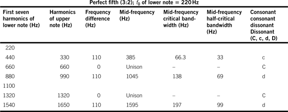
If they are in unison (equal frequencies) they are “perfectly consonant,” shown as “C” (note that their frequency difference is less than 5% of the critical bandwidth).
If their frequency difference is greater than the critical bandwidth of the frequency midway between them (i.e., the entry in column 3 is greater than that in column 5) they are “consonant,” shown as “c.”
If their frequency difference is less than half the critical bandwidth of the frequency midway between them (i.e., the entry in column 3 is less than that in column 6) they are “highly dissonant,” shown as “D.”
If their frequency difference is less than the critical bandwidth of the frequency midway between them but greater than half that critical bandwidth (i.e., the entry in column 3 is less than that in column 5 and greater than that in column 6) they are “dissonant,” shown as “d.”

The contribution to dissonance depends on where the musical interval occurs between adjacent harmonics in the natural harmonic series. The higher up the series it occurs, the greater the dissonant contribution made by harmonics of the two notes concerned. The case of a two-note unison is trivial in that all harmonics are in unison with each other and all contribute as “C.” For the octave, all harmonics of the upper note are in unison with harmonics of the lower note contributions as “C.” Tables 3.6–3.10 show the contribution to dissonance and consonance for the intervals perfect fifth (3:2), perfect fourth (4:3), major third (5:4), minor third (6:5) and major whole tone (9:8) respectively. The dissonance of the chord in each case is related to the entries in the final column which indicate increased dissonance in the order C, c, d and D; it can be seen that the dissonance increases as the harmonic number increases and the musical interval decreases.

Table 3.7 The degree of consonance and dissonance of a two-note chord in which all harmonics are present for both notes a perfect fourth apart, the f₀ for the lower note being 220 Hz

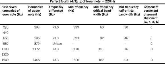
Table 3.8 The degree of consonance and dissonance of a two-note chord in which all harmonics are present for both notes a major third apart, the f₀ for the lower note being 220 Hz

Table 3.9 The degree of consonance and dissonance of a two-note chord in which all harmonics are present for both notes a minor third apart, the f₀ for the lower note being 220 Hz

Table 3.10 The degree of consonance and dissonance of a two-note chord in which all harmonics are present for both notes a major whole tone apart, the f₀ for the lower note being 220 Hz

The harmonics which are in unison with each other can be predicted from the harmonic number. For example, in the case of the perfect fourth the fourth harmonic of the lower note is in unison with the third of the upper note because their f₀ values are in the ratio (4:3). For the major whole tone (9:8), the unison will occur between harmonics (the eighth of the upper note and the ninth of the lower) which are not resolved by the auditory system for each individual note.

As a final point, the degree of dissonance of a given musical interval will vary depending on the f₀ value of the lower note, due to the nature of the critical bandwidth with center frequency (e.g., see Figure 3.8). Tables 3.11 and 3.12 illustrate this effect for the major third where the f₀ of the lower note is one octave and two octaves below that used in Table 3.8 at 110 Hz and 55 Hz respectively. The number of “D” entries increases in each case as the f₀ values of the two notes are lowered.

Table 3.11 The degree of consonance and dissonance of a two-note chord in which all harmonics are present for both notes a major third apart, the f₀ for the lower note being 110 Hz

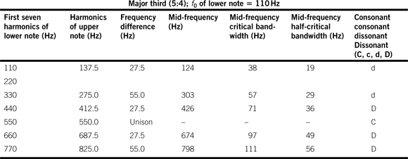
Table 3.12 The degree of consonance and dissonance of a two-note chord in which all harmonics are present for both notes a major third apart, the f₀ for the lower note being 55.0 Hz

This increase in dissonance of any given interval, excluding the unison and octave which are equally consonant at any pitch on this basis, manifests itself in terms of preferred chord spacings in classical harmony. As a rule when writing four-part harmony such as SATB (soprano, alto, tenor, bass) hymns, the bass and tenor parts are usually no closer together than a fourth except when they are above the bass staff, because the result would otherwise sound “muddy” or “harsh.”

Figure 3.17 shows a chord of C major in a variety of four-part spacings and inversions which illustrate this effect when the chords are played, preferably on an instrument producing a continuous steady sound for each note such as a pipe organ, instrumental group or suitable synthesizer sound. To realize the importance of this point, it is essential to listen to the effect. The psychoacoustics of music is, after all, about how music is perceived, not what it looks like on paper!

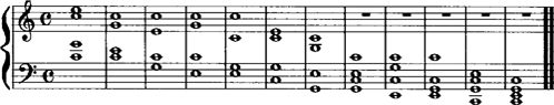
Figure 3.17 Different spacings of the chord of C major. Play each chord and listen to the degree of “muddiness” or “harshness” each produces (see text).

3.4 Tuning Systems

Musical scales are basic to most Western music. Modern keyboard instruments have 12 notes per octave with a musical interval of one semitone between adjacent notes. All common Western scales incorporate octaves whose frequency ratios are (2:1). Therefore it is only necessary to consider notes in a scale over a range of one octave, since the frequencies of notes in other octaves can be found from them. Early scales were based on one or more of the musical intervals found between members of the natural harmonic series (e.g. see Figure 3.3).

3.4.1 Pythagorean Tuning

The Pythagorean scale is built up from the perfect fifth. Starting, for example, from the note C and going up in 12 steps of a perfect fifth produces the “circle of fifths:” C, G, D, A, E, B, F#, C#, G#, D#, A#, E#, c. The final note after 12 steps around the circle of fifths, shown as c, has a frequency ratio to the starting note, C, of the frequency ratio of the perfect fifth (3:2) multiplied by itself 12 times, or:

An interval of 12 fifths is equivalent to seven octaves, and the frequency ratio for the note (c′) which is seven octaves above C is:

Thus 12 perfect fifths (C to c) is slightly sharp compared with seven octaves (C to c′) of the so-called “Pythagorean comma” which has a frequency ratio:

If the circle of fifths were established by descending by perfect fifths instead of ascending, the resulting note 12 fifths below the starting notes would be flatter than seven octaves by 1.0136433, and every note of the descending circle would be slightly different from the members of the ascending circle. Figure 3.18 shows this effect and the manner in which the notes can be notated. For example, notes such as D# and Eb, A# and Bb, Bbb and A are not the same and are known as “enharmonics,” giving rise to the pairs of intervals such as major third and diminished fourth, and major seventh and diminished octave shown in Figure 3.15. The Pythagorean scale can be built up on the starting note C by making F and G an exact perfect fourth and perfect fifth respectively (maintaining a perfect relationship for the sub-dominant and dominant respectively):

Figure 3.18 The Pythagorean scale is based on the circle of fifths formed either by ascending by 12 perfect fifths (outer) or descending by 12 perfect fifths (inner).

The frequency ratios for the other notes of the scale are found by ascending in perfect fifths from G and, when necessary, bringing the result down to be within an octave of the starting note. The resulting frequency ratios relative to the starting note C are:

The frequency ratios of the members of the Pythagorean major scale are shown in Figure 3.19 relative to C for convenience. The frequency ratios between adjacent notes can be calculated by dividing the frequency ratios of the upper note of the pair to C by that of the lower. For example:

Figure 3.19 Frequency ratios between the notes of a C major Pythagorean scale and the tonic (C).

Figure 3.18 shows the frequency ratios between adjacent notes of the Pythagorean major scale. A major scale consists of the following intervals: tone, tone, semitone, tone, tone, tone, semitone, and it can be seen that:

3.4.2 Just Tuning

Another important scale is the “just diatonic” scale which is made by keeping the intervals that make up the major triads pure: the octave (2:1), the perfect fifth (3:2) and the major third (5:4) for triads on the tonic, dominant and sub-dominant. The dominant and sub-dominant keynotes are a perfect fifth above and below the key note respectively. This produces all the notes of the major scale (any of which can be harmonized using one of these three chords). Taking the note C being used as a starting reference for convenience, the major scale is built as follows. The notes E and G are a major third (5:4) and a perfect fifth (3:2) respectively above the tonic, C:

The frequency ratios of B and D are a major third (5:4) and a perfect fifth (3:2) respectively above the dominant, G, and they are related to C as:

(The result for the D is brought down one octave to keep it within an octave of the C.)

The frequency ratios of A and C are a major third (5:4) and a perfect fifth (3:2) respectively above the sub-dominant F. The F is therefore a perfect fourth (4:3) above the C (perfect fourth plus a perfect fifth is an octave):

The “just diatonic” scale has both a major and a minor whole tone.

The frequency ratios of the members of the just diatonic major scale are shown in Figure 3.20 relative to C for convenience, along with the frequency ratios between adjacent notes (calculated by dividing the frequency ratio of the upper note of each pair to C by that of the lower). The figure shows that the just diatonic major scale (tone, tone, semitone, tone, tone, tone, semitone) has equal semitone intervals, but two different tone intervals, the larger of which is known as a “major whole tone” and the smaller as a “minor whole tone:”

Figure 3.20 Frequency ratios between the notes of a C major “just diatonic” scale and the tonic (C).

The two whole tone and the semitone intervals appear as members of the musical intervals between adjacent members of the natural harmonic series (see Figure 3.3), which means that the notes of the scale are as consonant with each other as possible for both melodic and harmonic musical phrases. However, the presence of two whole tone intervals means that this scale can only be used in one key since each key requires its own tuning. This means, for example, that the interval between D and A is:

which is a musically flatter fifth than the perfect fifth (3:2).

In order to tune a musical instrument for practical purposes to enable it to be played in a number of different keys, the Pythagorean comma has to be distributed among some of the fifths in the circle of fifths such that the note reached after 12 fifths is exactly seven octaves above the starting note (see Figure 3.18). This can be achieved by flattening some of the fifths, possibly by different amounts, while leaving some perfect, or flattening all of the fifths by varying amounts, or even by additionally sharpening some and flattening others to compensate. There is therefore an infinite variety of possibilities, but none will result in just tuning in all keys. Many tuning systems were experimented with to provide tuning of thirds and fifths which were close to just tuning in some keys at the expense of other keys whose tuning could end up being so out-of-tune as to be unusable musically.

Padgham (1986) gives a fuller discussion of tuning systems. A number of keyboard instruments have been experimented with which had split black notes (in either direction) to provide access to their enharmonics, giving C# and Db, D# and Eb, F# and Gb, G# and Ab, and A# and Bb—for example, the McClure pipe organ in the Faculty of Music at the University of Edinburgh discussed by Padgham (1986)—but these have never become popular with keyboard players.

3.4.3 Equal Tempered Tuning

The spreading of the Pythagorean comma unequally among the fifths in the circle results in an “unequal temperament.” Another possibility is to spread it evenly to give “equal temperament”, which makes modulation to all keys possible where each one is equally out-of-tune with the just scale. This is the tuning system commonly found on today’s keyboard instruments. All semitones are equal to one twelfth of an octave. Therefore the frequency ratio (r) for an equal tempered semitone is a number which when multiplied by itself 12 times is equal to 2, or:

A cent is one hundredth of a semitone.

The equal tempered semitone is subdivided into “cents,” where one cent is one hundredth of an equal tempered semitone. The frequency ratio for one cent (c) is therefore:

Cents are widely used in discussions of pitch intervals and the results of psychoacoustic experiments involving pitch. Appendix 3 gives an equation for converting frequency ratios to cents and vice versa.

Music can be played in all keys when equal tempered tuning is used, as all semitones and tones have identical frequency ratios. However, no interval is in-tune in relation to the intervals between adjacent members of the natural harmonic series (see Figure 3.3); therefore none is perfectly consonant. However, intervals of the equal tempered scale can still be considered in terms of their consonance and dissonance, because although harmonics of pairs of notes that are in unison for pure intervals (see Tables 3.6 to 3.12) are not identical in equal temperament, the difference is within the 5% critical bandwidth criterion for consonance. Beats (see Figure 2.6) will exist between some harmonics in equal tempered chords which are not present in their pure counterparts.

In today’s equal tempered scale, no interval is in-tune with integer ratios between frequencies except the octave.

Figure 3.21 shows the f₀ values and the note naming convention used in this book for eight octaves, four either side of middle C, tuned in equal temperament with a tuning reference of 440 Hz for A4: the A above middle C. The equal tempered system is found on modern keyboard instruments, but there is increasing interest among performing musicians and listeners alike in the use of unequal temperament. This may involve the use of original instruments or electronic synthesizers which incorporate various tuning systems. Padgham (1986) lists approximately 100 pipe organs in Britain which are tuned to an unequal temperament in addition to the McClure organ.

References

Howard, D.M., Hirson, A., Brookes, T., Tyrrell, A.M., 1995. Spectrography of disputed speech samples by peripheral human hearing modeling. Forensic Linguist. 2 (1), 28–38.

Moore, B.C.J., 1982. An Introduction to the Psychology of Hearing. Academic Press, London.

Padgham, C.A., 1986. The Well-tempered Organ. Positif Press, Oxford

Parkin, P.H., 1974. Pitch change during reverberant decay. J. Sound Vib. 32, 530.

Pickles, J.O., 1982. An Introduction to the Physiology of Hearing. Academic Press, London.

Plomp, R., Levelt, W.J.M., 1965. Tonal consonance and critical bandwidth. J. Acoust. Soc. Am. 38, 548.

Roederer, J.G., 1975. Introduction to the Physics and Psychophysics of Music. Springer-Verlag, New York.

Rossing, T.D., 2001. The Science of Sound, Third edition. Addison Wesley, New York.

Schouten, J.F., 1940. The perception of pitch. Philips Tech. Rev. 5, 286

Wever, E.G., 1949. Theory of Hearing. Wiley, New York

Zwicker, E., Flottorp, G., Stevens, S.S., 1957. Critical bandwidth in loudness summation. J. Acoust. Soc. Am. 29, 548.

¹His first law being basic to electrical work: voltage = current × resistance.

..................Content has been hidden....................

You can't read the all page of ebook, please click here login for view all page.

Table of Contents for Chapter 3: Notes and Harmony

Create new playlist

Sign In

Sign Up

Table of Contents for
Chapter 3: Notes and Harmony