
4
SUBSPACE TRACKING FOR SIGNAL PROCESSING
TELECOM SudParis, Evry, France
4.1 INTRODUCTION
Research in subspace and component-based techniques originated in statistics in the middle of the last century through the problem of linear feature extraction solved by the Karhunen–Loeve Transform (KLT). It began to be applied to signal processing 30 years ago and considerable progress has since been made. Thorough studies have shown that the estimation and detection tasks in many signal processing and communications applications such as data compression, data filtering, parameter estimation, pattern recognition, and neural analysis can be significantly improved by using the subspace and component-based methodology. Over the past few years new potential applications have emerged, and subspace and component methods have been adopted in several diverse new fields such as smart antennas, sensor arrays, multiuser detection, time delay estimation, image segmentation, speech enhancement, learning systems, magnetic resonance spectroscopy, and radar systems, to mention only a few examples. The interest in subspace and component-based methods stems from the fact that they consist in splitting the observations into a set of desired and a set of disturbing components. They not only provide new insights into many such problems, but they also offer a good tradeoff between achieved performance and computational complexity. In most cases they can be considered to be low-cost alternatives to computationally intensive maximum-likelihood approaches.
In general, subspace and component-based methods are obtained by using batch methods, such as the eigenvalue decomposition (EVD) of the sample covariance matrix or the singular value decomposition (SVD) of the data matrix. However, these two approaches are not suitable for adaptive applications for tracking nonstationary signal parameters, where the required repetitive estimation of the subspace or the eigenvectors can be a real computational burden because their iterative implementation needs O(n3) operations at each update, where n is the dimension of the vector-valued data sequence. Before proceeding with a brief literature review of the main contributions of adaptive estimation of subspace or eigenvectors, let us first classify these algorithms with respect to their computational complexity. If r denotes the rank of the principal or dominant or minor subspace we would like to estimate, since usually r « n, it is traditional to refer to the following classification. Algorithms requiring O(n2r) or O(n2) operations by update are classified as high complexity; algorithms with O(nr2) operations as medium complexity and finally, algorithms with O(nr) operations as low complexity. This last category constitutes the most important one from a real time implementation point of view, and schemes belonging to this class are also known in the literature as fast subspace tracking algorithms. It should be mentioned that methods belonging to the high complexity class usually present faster convergence rates compared to the other two classes. From the paper by Owsley [56], that first introduced an adaptive procedure for the estimation of the signal subspace with O(n2r) operations, the literature referring to the problem of subspace or eigenvectors tracking from a signal processing point of view is extremely rich. The survey paper [20] constitutes an excellent review of results up to 1990, treating the first two classes, since the last class was not available at the time it was written. The most popular algorithm of the medium class was proposed by Karasalo in [40]. In [20], it is stated that this dominant subspace algorithm offers the best performance to cost ratio and thus serves as a point of reference for subsequent algorithms by many authors. The merger of signal processing and neural networks in the early 1990s [39] brought much attention to a method originated by Oja [50] and applied by many others. The Oja method requires only O(nr) operations at each update. It is clearly the continuous interest in the subject and significant recent developments that gave rise to this third class. It is outside of the scope of this chapter to give a comprehensive survey of all the contributions, but rather to focus on some of them. The interested reader may refer to [29, pp. 30–43] for an exhaustive literature review and to [8] for tables containing exact computational complexities and ranking with respect to the convergence of recent subspace tracking algorithms. In the present work, we mainly emphasize the low complexity class for both dominant and minor subspace, and dominant and minor eigenvector tracking, while we briefly address the most important schemes of the other two classes. For these algorithms, we will focus on their derivation from different iterative procedures coming from linear algebra and on their theoretical convergence and performance in stationary environments. Many important issues such as the finite precision effects on their behavior (e.g. possible numerical instabilities due to roundoff error accumulation), the different adaptive stepsize strategies and the tracking capabilities of these algorithms in nonstationary environments will be left aside. The interested reader may refer to the simulation sections of the different papers that deal with these issues.
The derivation and analysis of algorithms for subspace tracking requires a minimum background in linear algebra and matrix analysis. This is the reason why in Section 2, standard linear algebra materials necessary for this chapter are recalled. This is followed in Section 3 by the general studied observation model to fix the main notations and by the statement of the adaptive and tracking of principal or minor subspaces (or eigenvectors) problems. Then, Oja's neuron is introduced in Section 4 as a preliminary example to show that the subspace or component adaptive algorithms are derived empirically from different adaptations of standard iterative computational techniques issued from numerical methods. In Sections 5 and 6 different adaptive algorithms for principal (or minor) subspace and component analysis are introduced respectively. As for Oja's neuron, the majority of these algorithms can be viewed as some heuristic variations of the power method. These heuristic approaches need to be validated by convergence and performance analysis. Several tools such as the stability of the ordinary differential equation (ODE) associated with a stochastic approximation algorithm and the Gaussian approximation to address these points in a stationary environment are given in Section 7. Some illustrative applications of principal and minor subspace tracking in signal processing are given in Section 8. Section 9 contains some concluding remarks. Finally, some exercises are proposed in Section 10, essentially to prove some properties and relations introduced in the other sections.
4.2 LINEAR ALGEBRA REVIEW
In this section several useful notions coming from linear algebra as the EVD, the QR decomposition and the variational characterization of eigenvalues/eigenvectors of real symmetric matrices, and matrix analysis as a class of standard subspace iterative computational techniques are recalled. Finally a characterization of the principal subspace of a covariance matrix derived from the minimization of a mean square error will complete this section.
4.2.1 Eigenvalue Value Decomposition
Let C be an n × n real symmetric [resp. complex Hermitian] matrix, which is also non-negative definite because C will represent throughout this chapter a covariance matrix. Then, there exists (see e.g. [37, Sec. 2.5]) an orthonormal [resp. unitary] matrix U = [u1,…, un] and a real diagonal matrix Δ = Diag(λ1, …, λn) such that C can be decomposed1 as follows

The diagonal elements of Δ are called eigenvalues and arranged in decreasing order, satisfy λ1 ≥ … ≥ λn > 0, while the orthogonal columns (ui)i=1,…, n of U are the corresponding unit 2-norm eigenvectors of C.
For the sake of simplicity, only real-valued data will be considered from the next subsection and throughout this chapter. The extension to complex-valued data is often straightforward by changing the transposition operator to the conjugate transposition one. But we note two difficulties. First, for simple2 eigenvalues, the associated eigenvectors are unique up to a multiplicative sign in the real case, but only to a unit modulus constant in the complex case, and consequently a constraint ought to be added to fix them to avoid any discrepancies between the statistics observed in numerical simulations and the theoretical formulas. The reader interested by the consequences of this nonuniqueness on the derivation of the asymptotic variance of estimated eigenvectors from sample covariance matrices (SCMs) can refer to [34], (see also Exercise 4.1). Second, in the complex case, the second-order properties of multidimensional zero-mean random variables x are not characterized by the complex Hermitian covariance matrix E(xxH) only, but also by the complex symmetric complementary covariance [58] matrix E(xxT).
The computational complexity of the most efficient existing iterative algorithms that perform EVD of real symmetric matrices is cubic by iteration with respect to the matrix dimension (more details can be sought in [35, Chap. 8]).
4.2.2 QR Factorization
The QR factorization of an n × r real-valued matrix W, with n ≥ r is defined as (see e.g. [37, Sec. 2.6])
![]()
where Q is an n × n orthonormal matrix, R is an n × r upper triangular matrix, and Q1 denotes the first r columns of Q and R1 the r × r matrix constituted with the first r rows of R. If W is of full column rank, the columns of Q1 form an orthonormal basis for the range of W. Furthermore, in this case the skinny factorization Q1R1 of W is unique if R1 is constrained to have positive diagonal entries. The computation of the QR decomposition can be performed in several ways. Existing methods are based on Householder, block Householder, Givens or fast Givens transformations. Alternatively, the Gram–Schmidt orthonormalization process or a more numerically stable variant called modified Gram–Schmidt can be used. The interested reader can seek details for the aforementioned QR implementations in [35, pp. 224–233]), where the complexity is of the order of O(nr2) operations.
4.2.3 Variational Characterization of Eigenvalues/Eigenvectors of Real Symmetric Matrices
The eigenvalues of a general n × n matrix C are only characterized as the roots of the associated characteristic equation. But for real symmetric matrices, they can be characterized as the solutions to a series of optimization problems. In particular, the largest λ1 and the smallest λn eigenvalues of C are solutions to the following constrained maximum and minimum problem (see e.g. [37, Sec. 4.2]).
![]()
Furthermore, the maximum and minimum are attained by the unit 2-norm eigenvectors u1 and un associated with λ1 and λn respectively, which are unique up to a sign for simple eigenvalues λ1 and λn. For nonzero vectors ![]() , the expression
, the expression ![]() is known as the Rayleigh's quotient and the constrained maximization and minimization (4.3) can be replaced by the following unconstrained maximization and minimization
is known as the Rayleigh's quotient and the constrained maximization and minimization (4.3) can be replaced by the following unconstrained maximization and minimization
![]()
For simple eigenvalues λ1, λ2, …, λr or λn, λn−1, …, λn−r+1, (4.3) extends by the following iterative constrained maximizations and minimizations (see e.g. [37, Sec. 4.2])
![]()
![]()
and the constrained maximum and minimum are attained by the unit 2-norm eigenvectors uk associated with λk which are unique up to a sign.
Note that when λr > λr+1 or λn−r > λn−r+1, the following global constrained maximizations or minimizations (denoted subspace criterion)

or
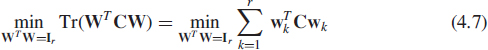
where W = [w1, …, wr] is an arbitrary n × r matrix, have four solutions (see e.g. [70] and Exercise 4.6), W = [u1, …, ur]Q or W = [un−r+1, …, un]Q respectively, where Q is an arbitrary r × r orthogonal matrix. Thus, subspace criterion (4.7) determines the subspace spanned by {u1, …, ur} or {un−r+1, …, un}, but does not specify the basis of this subspace at all.
Finally, when now, λ1 > λ2 > … > λr > λr+1 or λn−r > λn−r+1 > … > λn−1 > λn,3 if (ωk)k=1, … r denotes r arbitrary positive and different real numbers such that ω1 > ω2 > … > ωr > 0, the following modification of subspace criterion (4.7) denoted weighted subspace criterion
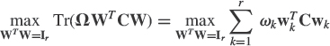
or

with Ω = Diag(ω1, …, ωr), has [54] the unique solution {±u1, …, ±ur} or {±un−r+1, …, ±un}, respectively.
4.2.4 Standard Subspace Iterative Computational Techniques
The first subspace problem consists in computing the eigenvector associated with the largest eigenvalue. The power method presented in the sequel is the simplest iterative techniques for this task. Under the condition that λ1 is the unique dominant eigenvalue associated with u1 of the real symmetric matrix C, and starting from arbitrary unit 2-norm w0 not orthogonal to u1, the following iterations produce a sequence (αi, wi) that converges to the largest eigenvalue λ1 and its corresponding eigenvector unit 2-norm ±u1.

The proof can be found in [35, p. 406], where the definition and the speed of this convergence are specified in the following. Define θi ∈ [0, π/2] by ![]() satisfying cos(θ0) ≠ 0, then
satisfying cos(θ0) ≠ 0, then

Consequently the convergence rate of the power method is exponential and proportional to the ratio ![]() for the eigenvector and to
for the eigenvector and to ![]() for the associated eigenvalue. If w0 is selected randomly, the probability that this vector is orthogonal to u1 is equal to zero. Furthermore, if w0 is deliberately chosen orthogonal to u1, the effect of finite precision in arithmetic computations will introduce errors that will finally provoke the loss of this orthogonality and therefore convergence to ±u1.
for the associated eigenvalue. If w0 is selected randomly, the probability that this vector is orthogonal to u1 is equal to zero. Furthermore, if w0 is deliberately chosen orthogonal to u1, the effect of finite precision in arithmetic computations will introduce errors that will finally provoke the loss of this orthogonality and therefore convergence to ±u1.
Suppose now that C nonnegative. A straightforward generalization of the power method allows for the computation of the r eigenvectors associated with the r largest eigenvalues of C when its first r+ 1 eigenvalues are distinct, or of the subspace corresponding to the r largest eigenvalues of C when λr > λr+1 only. This method can be found in the literature under the name of orthogonal iteration, for example, in [35], subspace iteration, for example, in [57] or simultaneous iteration method, for example, in [64]. First, consider the case where the r + 1 largest eigenvalues of C are distinct. With ![]() and Δr = Diag(λ1, …, λr), the following iterations produce a sequence (Λi, Wi) that converges to (Δr, [±u1, …, ±ur]).
and Δr = Diag(λ1, …, λr), the following iterations produce a sequence (Λi, Wi) that converges to (Δr, [±u1, …, ±ur]).
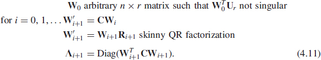
The proof can be found in [35, p. 411]. The definition and the speed of this convergence are similar to those of the power method, it is exponential and proportional to ![]() for the eigenvectors and to
for the eigenvectors and to ![]() for the eigenvalues. Note that if r = 1, then this is just the power method. Moreover for arbitrary r, the sequence formed by the first column of Wi is precisely the sequence of vectors produced by the power method with the first column of W0 as starting vector.
for the eigenvalues. Note that if r = 1, then this is just the power method. Moreover for arbitrary r, the sequence formed by the first column of Wi is precisely the sequence of vectors produced by the power method with the first column of W0 as starting vector.
Consider now the case where λr > λr+1. Then the following iteration method

where the orthonormalization (Orthonorm) procedure not necessarily given by the QR factorization, generates a sequence Wi that converges to the dominant subspace generated by {u1, …, ur} only. This means precisely that the sequence ![]() (which here is a projection matrix because
(which here is a projection matrix because ![]() ) converges to the projection matrix
) converges to the projection matrix ![]() . In the particular case where the QR factorization is used in the orthonormalization step, the speed of this convergence is exponential and proportional to
. In the particular case where the QR factorization is used in the orthonormalization step, the speed of this convergence is exponential and proportional to ![]() , that is, more precisely [35, p. 411]
, that is, more precisely [35, p. 411]
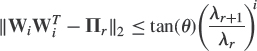
where ![]() is specified by
is specified by ![]() . This type of convergence is very specific. The r orthonormal columns of Wi do not necessary converge to a particular orthonormal basis of the dominant subspace generated by u1, …, ur, but may eventually rotate in this dominant subspace as i increases. Note that the orthonormalization step (4.12) can be realized by other means than the QR decomposition. For example, extending the r = 1 case
. This type of convergence is very specific. The r orthonormal columns of Wi do not necessary converge to a particular orthonormal basis of the dominant subspace generated by u1, …, ur, but may eventually rotate in this dominant subspace as i increases. Note that the orthonormalization step (4.12) can be realized by other means than the QR decomposition. For example, extending the r = 1 case
![]()
to arbitrary r, yields
![]()
where the square root inverse of the matrix ![]() is defined by the EVD of the matrix with its eigenvalues replaced by their square root inverses. The speed of convergence of the associated algorithm is exponential and proportional to
is defined by the EVD of the matrix with its eigenvalues replaced by their square root inverses. The speed of convergence of the associated algorithm is exponential and proportional to ![]() as well [38].
as well [38].
Finally, note that the power and the orthogonal iteration methods can be extended to obtain the minor subspace or eigenvectors by replacing the matrix C by In − μC where 0 < μ< 1/λ1 such that the eigenvalues 1 − μλn > … ≥ 1 − μλ1 > 0 of In − μC are strictly positive.
4.2.5 Characterization of the Principal Subspace of a Covariance Matrix from the Minimization of a Mean Square Error
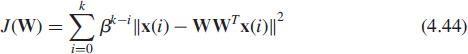
In the particular case where the matrix C is the covariance of the zero-mean random variable x, consider the scalar function J(W) where W denotes an arbitrary n × r matrix
![]()
The following two properties are proved (e.g. see [71] and Exercises 4.7 and 4.8).
First, the stationary points W of J(W) [i.e., the points W that cancel J(W)] are given by W = UrQ where the r columns of Ur denotes here arbitrary r distinct unit-2 norm eigenvectors among u1, …, un of C and where Q is an arbitrary r × r orthogonal matrix. Furthermore at each stationary point, J(W) equals the sum of eigenvalues whose eigenvectors are not included in Ur.
Second, in the particular case where λr > λr+1, all stationary points of J(W) are saddle points except the points W whose associated matrix Ur contains the r dominant eigenvectors u1, …, ur of C. In this case J(W) attains the global minimum ![]() . It is important to note that at this global minimum, W does not necessarily contain the r dominant eigenvectors u1, …, ur of C, but rather an arbitrary orthogonal basis of the associated dominant subspace. This is not surprising because
. It is important to note that at this global minimum, W does not necessarily contain the r dominant eigenvectors u1, …, ur of C, but rather an arbitrary orthogonal basis of the associated dominant subspace. This is not surprising because
![]()
with Tr(WTCW) = Tr(CWWT) and thus J(W) is expressed as a function of W through WWT which is invariant with respect to rotation WQ of W. Finally, note that when r = 1 and λ1 > λ2, the solution of the minimization of J(w) (4.14) is given by the unit 2-norm dominant eigenvector ±u1.
4.3 OBSERVATION MODEL AND PROBLEM STATEMENT
4.3.1 Observation Model
The general iterative subspace determination problem described in the previous section, will be now specialized to a class of matrices C computed from observation data. In typical applications of subspace-based signal processing, a sequence4 of data vectors ![]() is observed, satisfying the following very common observation signal model
is observed, satisfying the following very common observation signal model
![]()
where s(k) is a vector containing the information signal lying on an r-dimensional linear subspace of ![]() with r < n, while n(k) is a zero-mean additive random white noise (AWN) random vector, uncorrelated from s(k). Note that s(k) is often given by s(k) = A(k)r(k) where the full rank n × r matrix A(k) is deterministically parameterized and r(k) is a r-dimensional zero-mean full random vector (i.e., with E[r(k)rT(k)] nonsingular). The signal part s(k) may also randomly select among r deterministic vectors. This random selection does not necessarily result in a zero-mean signal vector s(k).
with r < n, while n(k) is a zero-mean additive random white noise (AWN) random vector, uncorrelated from s(k). Note that s(k) is often given by s(k) = A(k)r(k) where the full rank n × r matrix A(k) is deterministically parameterized and r(k) is a r-dimensional zero-mean full random vector (i.e., with E[r(k)rT(k)] nonsingular). The signal part s(k) may also randomly select among r deterministic vectors. This random selection does not necessarily result in a zero-mean signal vector s(k).
In these assumptions, the covariance matrix Cs(k) of s(k) is r-rank deficient and
![]()
where ![]() denotes the AWN power. Taking into account that Cs(k) is of rank r and applying the EVD (4.1) on Cx(k) yields
denotes the AWN power. Taking into account that Cs(k) is of rank r and applying the EVD (4.1) on Cx(k) yields

where the n × r and n × (n − r) matrices Us(k) and Un(k) are orthonormal bases for the denoted signal or dominant and noise or minor subspace of Cx(k) and Δs(k) is a r × r diagonal matrix constituted by the r nonzero eigenvalues of Cs(k). We note that the column vectors of Us(k) are generally unique up to a sign, in contrast to the column vectors of Un(k) for which Un(k) is defined up to a right multiplication by a (n − r) × (n − r) orthonormal matrix Q. However, the associated orthogonal projection matrices ![]() and
and ![]() respectively denoted signal or dominant projection matrices and noise or minor projection matrices that will be introduced in the next sections are both unique.
respectively denoted signal or dominant projection matrices and noise or minor projection matrices that will be introduced in the next sections are both unique.
4.3.2 Statement of the Problem
A very important problem in signal processing consists in continuously updating the estimate Us(k), Un(k), Πs(k) or Πn(k) and sometimes with Δs(k) and ![]() , assuming that we have available consecutive observation vectors x(i), i = …, k − 1, k, … when the signal or noise subspace is slowly time-varying compared to x(k). The dimension r of the signal subspace may be known a priori or estimated from the observation vectors. A straightforward way to come up with a method that solves these problems is to provide efficient adaptive estimates C(k) of Cx(k) and simply apply an EVD at each time step k. Candidates for this estimate C(k) are generally given by sliding windowed sample data covariance matrices when the sequence of Cx(k) undergoes relatively slow changes. With an exponential window, the estimated covariance matrix is defined as
, assuming that we have available consecutive observation vectors x(i), i = …, k − 1, k, … when the signal or noise subspace is slowly time-varying compared to x(k). The dimension r of the signal subspace may be known a priori or estimated from the observation vectors. A straightforward way to come up with a method that solves these problems is to provide efficient adaptive estimates C(k) of Cx(k) and simply apply an EVD at each time step k. Candidates for this estimate C(k) are generally given by sliding windowed sample data covariance matrices when the sequence of Cx(k) undergoes relatively slow changes. With an exponential window, the estimated covariance matrix is defined as
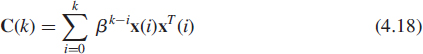
where 0 < β < 1 is the forgetting factor. Its use is intended to ensure that the data in the distant past are downweighted in order to afford the tracking capability when we operate in a nonstationary environment. C(k) can be recursively updated according to the following scheme
![]()
Note that
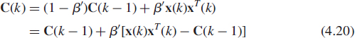
is also used. These estimates C(k) tend to smooth the variations of the signal parameters and so are only suitable for slowly changing signal parameters. For sudden signal parameter changes, the use of a truncated window may offer faster tracking. In this case, the estimated covariance matrix is derived from a window of length l
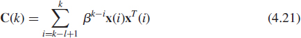
where 0 < β ≤ 1. The case β = 1 corresponds to a rectangular window. This matrix can be recursively updated according to the following scheme
![]()
Both versions require O(n2) operations with the first having smaller computational complexity and memory needs. Note that for β = 0, (4.22) gives the coarse estimate x(k)xT(k) of Cx(k) as used in the least mean square (LMS) algorithms for adaptive filtering (see e.g. [36]).
Applying an EVD on C(k) at each time k is of course the best possible way to estimate the eigenvectors or subspaces we are looking for. This approach is known as direct EVD and has high complexity which is O(n3). This method usually serves as point of reference when dealing with the different less computationally demanding approaches described in the next sections. These computationally efficient algorithms will compute signal or noise eigenvectors (or signal or noise projection matrices) at the time instant k + 1 from the associated estimate at time k and the new arriving sample vector x(k).
4.4 PRELIMINARY EXAMPLE: OJA'S NEURON
Let us introduce these adaptive procedures by a simple example: The following Oja's neuron originated by Oja [50] and then applied by many others that estimates the eigenvector associated with the unique largest eigenvalue of a covariance matrix of the stationary vector x(k).
![]()
The first term on the right side is the previous estimate of ±u1, which is kept as a memory of the iteration. The whole term in brackets is the new information. This term is scaled by the stepsize μ and then added to the previous estimate w(k) to obtain the current estimate w(k+ 1). We note that this new information is formed by two terms. The first one x(k)xT(k)w(k) contains the first step of the power method (4.9) and the second one is simply the previous estimate w(k) adjusted by the scalar wT(k)x(k)xT(k)w(k) so that these two terms are on the same scale. Finally, we note that if the previous estimate w(k) is already the desired eigenvector ±u1, the expectation of this new information is zero, and hence, w(k + 1) will be hovering around ±u1. The step size μ controls the balance between the past and the new information. Introduced in the neural networks literature [50] within the framework of a new synaptic modification law, it is interesting to note that this algorithm can be derived from different heuristic variations of numerical methods introduced in Section 4.2.
First consider the variational characterization recalled in Subsection 4.2.3. Because ![]() , the constrained maximization (4.3) or (4.7) can be solved using the following constrained gradient-search procedure
, the constrained maximization (4.3) or (4.7) can be solved using the following constrained gradient-search procedure
in which the stepsize μ is sufficiency small enough. Using the approximation μ2«μ yields

Then, using the instantaneous estimate x(k)xT(k) of Cx(k), Oja's neuron (4.23) is derived.
Consider now the power method recalled in Subsection 4.2.4. Noticing that Cx and In+ μCx have the same eigenvectors, the step ![]() of (4.9) can be replaced by
of (4.9) can be replaced by ![]() and using the previous approximations yields Oja's neuron (4.23) anew.
and using the previous approximations yields Oja's neuron (4.23) anew.
Finally, consider the characterization of the eigenvector associated with the unique largest eigenvalue of a covariance matrix derived from the mean square error E(||x − wwTx||2) recalled in Subsection 4.2.5. Because
![]()
an unconstrained gradient-search procedure yields
![]()
Then, using the instantaneous estimate x(k)xT(k) of Cx(k) and the approximation wT(k)w(k) = 1 justified by the convergence of the deterministic gradient-search procedure to ±u1 when μ → 0, Oja's neuron (4.23) is derived again.
Furthermore, if we are interested in adaptively estimating the associated single eigenvalue λ1, the minimization of the scalar function ![]() by a gradient-search procedure can be used. With the instantaneous estimate x(k)xT(k) of Cx(k) and with the estimate w(k) of u1 given by (4.23), the following stochastic gradient algorithm is obtained.
by a gradient-search procedure can be used. With the instantaneous estimate x(k)xT(k) of Cx(k) and with the estimate w(k) of u1 given by (4.23), the following stochastic gradient algorithm is obtained.
![]()
We note that the previous two heuristic derivations could be extended to the adaptive estimation of the eigenvector associated with the unique smallest eigenvalue of Cx(k). Using the constrained minimization (4.3) or (4.7) solved by a constrained gradient-search procedure or the power method (4.9) where the step ![]() of (4.9) is replaced by
of (4.9) is replaced by ![]() (where 0 < μ < 1/λ1) yields (4.23) after the same derivation, but where the sign of the stepsize μ is reversed.
(where 0 < μ < 1/λ1) yields (4.23) after the same derivation, but where the sign of the stepsize μ is reversed.
![]()
The associated eigenvalue λn could be also derived from the minimization of ![]() and consequently obtained by (4.24) as well, where w(k) is issued from (4.25).
and consequently obtained by (4.24) as well, where w(k) is issued from (4.25).
These heuristic approaches are derived from iterative computational techniques issued from numerical methods recalled in Section 4.2, and need to be validated by convergence and performance analysis for stationary data x(k). These issues will be considered in Section 4.7. In particular it will be proved that the coupled stochastic approximation algorithms (4.23) and (4.24) in which the stepsize μ is decreasing, converge to the pair (±u1, λ1), in contrast to the stochastic approximation algorithm (4.25) that diverges. Then, due to the possible accumulation of rounding errors, the algorithms that converge theoretically must be tested through numerical experiments to check their numerical stability in stationary environments. Finally extensive Monte Carlo simulations must be carried out with various stepsizes, initialization conditions, SNRs, and parameters configurations in nonstationary environments.
4.5 SUBSPACE TRACKING
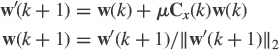
In this section, we consider the adaptive estimation of dominant (signal) and minor (noise) subspaces. To derive such algorithms from the linear algebra material recalled in Subsections 4.2.3, 4.2.4, and 4.2.5 similarly as for Oja's neuron, we first note that the general orthogonal iterative step (4.12): Wi+1 = Orthonorm{CWi} allows for the following variant for adaptive implementation
![]()
where μ > 0 is a small parameter known as stepsize, because In + μC has the same eigenvectors as C with associated eigenvalues (1 + μλi)i=1,…,n. Noting that In − μC has also the same eigenvectors as C with associated eigenvalues (1 − μλi)i=1,…, n, arranged exactly in the opposite order as (λi)i=1,…, n for μ sufficiently small (μ < 1/λ1), the general orthogonal iterative step (4.12) allows for the following second variant of this iterative procedure to converge to the r-dimensional minor subspace of C if λn−r > λn−r+1.
![]()
When the matrix C is unknown and, instead we have sequentially the data sequence x(k), we can replace C by an adaptive estimate C(k) (see Section 4.3.2). This leads to the adaptive orthogonal iteration algorithm
![]()
where the + sign generates estimates for the signal subspace (if λr > λr+1) and the − sign for the noise subspace (if λn−r > λn−r+1). Depending on the choice of the estimate C(k) and of the orthonormalization (or approximate orthonormalization), we can obtain alternative subspace tracking algorithms.
We note that maximization or minimization in (4.7) of ![]() subject to the constraint WTW = Ir can be solved by a constrained gradient-descent technique. Because
subject to the constraint WTW = Ir can be solved by a constrained gradient-descent technique. Because ![]() , we obtain the following Rayleigh quotient-based algorithm
, we obtain the following Rayleigh quotient-based algorithm
![]()
whose general expression is the same as general expression (4.26) derived from the orthogonal iteration approach. We will denote this family of algorithms as the power-based methods. It is interesting to note that a simple sign change enables one to switch from the dominant to the minor subspaces. Unfortunately, similarly to Oja's neuron, many minor subspace algorithms will be unstable or stable but non-robust (i.e., numerically unstable with a tendency to accumulate round-off errors until their estimates are meaningless), in contrast to the associated majorant subspace algorithms. Consequently, the literature of minor subspace tracking techniques is very limited as compared to the wide variety of methods that exists for the tracking of majorant subspaces.
4.5.1 Subspace Power-based Methods
Clearly the simplest selection for C(k) is the instantaneous estimate x(k)xT(k), which gives rise to the Data Projection Method (DPM) first introduced in [70] where the orthonormalization is performed using the Gram–Schmidt procedure.
![]()
In nonstationary situations, estimates (4.19) or (4.20) of the covariance Cx(k) of x(k) at time k have been tested in [70]. For this algorithm to converge, we need to select a stepsize μ such that μ « 1/λ1 (see e.g. [29]). To satisfy this requirement (in nonstationary situations included) and because most of the time we have Tr[Cx(k)] » λ1(k), the following two normalized step sizes have been proposed in [70]
![]()
where μ may be close to unity and where the choice of ν ∈ (0, 1) depends on the rapidity of the change of the parameters of the observation signal model (4.15). Note that a better numerical stability can be achieved [5] if μk is chosen, similar to the normalized LMS algorithm [36], as ![]() where α is a very small positive constant. Obviously, this algorithm (4.28) has very high computational complexity due to the Gram–Schmidt orthonormalization step.
where α is a very small positive constant. Obviously, this algorithm (4.28) has very high computational complexity due to the Gram–Schmidt orthonormalization step.
To reduce this computational complexity, many algorithms have been proposed. Going back to the DPM algorithm (4.28), we observe that we can write
![]()
where the matrix G(k + 1) is responsible for performing exact or approximate orthonormalization while preserving the space generated by the columns of ![]() . It is the different choices of G(k + 1) that will pave the way for alternative less computationally demanding algorithms. Depending on whether this orthonormalization is exact or approximate, two families of algorithms have been proposed in the literature.
. It is the different choices of G(k + 1) that will pave the way for alternative less computationally demanding algorithms. Depending on whether this orthonormalization is exact or approximate, two families of algorithms have been proposed in the literature.
The Approximate Symmetric Orthonormalization Family The columns of W′(k + 1) can be approximately orthonormalized in a symmetrical way. Since W(k) has orthonormal columns, for sufficiently small μk the columns of W′(k + 1) will be linearly independent, although not orthonormal. Then ![]() is positive definite, and W(k + 1) will have orthonormal columns if
is positive definite, and W(k + 1) will have orthonormal columns if ![]() (unique if G(k + 1) is constrained to be symmetric). A stochastic algorithm denoted Subspace Network Learning (SNL) and later Oja's algorithm have been derived in [53] to estimate dominant subspace. Assuming μk is sufficiency enough, G(k + 1) can be expanded in μk as follows
(unique if G(k + 1) is constrained to be symmetric). A stochastic algorithm denoted Subspace Network Learning (SNL) and later Oja's algorithm have been derived in [53] to estimate dominant subspace. Assuming μk is sufficiency enough, G(k + 1) can be expanded in μk as follows
Omitting second-order terms, the resulting algorithm reads5
![]()
The convergence of this algorithm has been earlier studied in [78] and then in [69], where it was shown that the solution W(t) of its associated ODE (see Subsection 4.7.1) need not tend to the eigenvectors {v1, …,vr}, but only to a rotated basis W*, of the subspace spanned by them. More precisely, it has been proved in [16] that under the assumption that W(0) is of full column rank such that its projection to the signal subspace of Cx is linearly independent, there exists a rotated basis W* of this signal subspace such that ![]() . A performance analysis has been given in [24, 25]. This issue will be used as an example analysis of convergence and performance in Subsection 4.7.3. Note that replacing x(k)xT(k) by βIn ±x(k)xT(k) (with β > 0) in (4.30), leads to a modified Oja's algorithm [15], which, not affecting its capability of tracking a signal subspace with the sign +, can track a noise subspace by changing the sign (if β > λ1). Of course, these modified Oja's algorithms enjoy the same convergence properties as Oja's algorithm (4.30).
. A performance analysis has been given in [24, 25]. This issue will be used as an example analysis of convergence and performance in Subsection 4.7.3. Note that replacing x(k)xT(k) by βIn ±x(k)xT(k) (with β > 0) in (4.30), leads to a modified Oja's algorithm [15], which, not affecting its capability of tracking a signal subspace with the sign +, can track a noise subspace by changing the sign (if β > λ1). Of course, these modified Oja's algorithms enjoy the same convergence properties as Oja's algorithm (4.30).
Many other modifications of Oja's algorithm have appeared in the literature, particularly to adapt it to noise subspace tracking. To obtain such algorithms, it is interesting to point out that, in general, it is not possible to obtain noise subspace tracking algorithms by simply changing the sign of the stepsize of a signal subspace tracking algorithm. For example, changing the sign in (4.30) or (4.85) leads to an unstable algorithm (divergence) as will be explained in Subsection 4.7.3 for r = 1. Among these modified Oja's algorithms, Chen et al. [16] have proposed the following unified algorithm
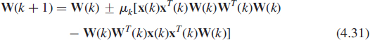
where the signs + and − are respectively associated with signal and noise tracking algorithms. While the associated ODE maintains WT(t)W(t) = Ir if WT(0)W(0) = Ir and enjoys [16] the same stability properties as Oja's algorithm, the stochastic approximation to algorithm (4.31) suffers from numerical instabilities (see e.g. the numerical simulations in [28]). Thus, its practical use requires periodic column reorthonormalization. To avoid these numerical instabilities, this algorithm has been modified [17] by adding the penalty term W(k)[In − W(k)WT(k)] to the field of (4.31). As far as noise subspace tracking is concerned, Douglas et al. [28] have proposed modifying the algorithm (4.31) by multiplying the first term of its field by WT(k)W(k) whose associated term in the ODE tends to Ir, viz
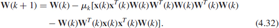
It is proved in [28] that the locally asymptotically stable points W of the ODE associated with this algorithm satisfy WTW = Ir and Span(W) = Span(Un). But the solution W(t) of the associated ODE does not converge to a particular basis W* of the noise subspace but rather, it is proved that Span[W(t)] tends to Span(Un) (in the sense that the projection matrix associated with the subspace Span[W(t)] tends to Πn). Numerical simulations presented in [28] show that this algorithm is numerically more stable than the minor subspace version of algorithm (4.31).
To eliminate the instability of the noise tracking algorithm derived from Oja's algorithm (4.30) where the sign of the stepsize is changed, Abed Meraim et al. [2] have proposed forcing the estimate W(k) to be orthonormal at each time step k (see Exercise 4.10) that can be used for signal subspace tracking (by reversing the sign of the stepsize) as well. But this algorithm converges with the same speed of convergence as Oja's algorithm (4.30). To accelerate its convergence, two normalized versions (denoted Normalized Oja's algorithm (NOja) and Normalized Orthogonal Oja's algorithm (NOOJa)) of this algorithm have been proposed in [4]. They can perform both signal and noise tracking by switching the sign of the stepsize for which an approximate closed-form expression has been derived. A convergence analysis of the NOja algorithm has been presented in [7] using the ODE approach. Because the ODE associated with the field of this stochastic approximation algorithm is the same as those associated with the projection approximation-based algorithm (4.43), it enjoys the same convergence properties.
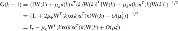
The Exact Orthonormalization Family The orthonormalization (4.29) of the columns of W′(k + 1) can be performed exactly at each iteration by the symmetric square root inverse of ![]() due to the fact that the latter is a rank one modification of the identity matrix
due to the fact that the latter is a rank one modification of the identity matrix
![]()
with ![]() and
and ![]() . Using the identity
. Using the identity
![]()
we obtain
![]()
with 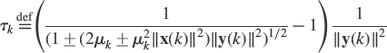 . Substituting (4.35) into (4.29) leads to
![]()
where ![]() . All these steps lead to the Fast Rayleigh quotient-based Adaptive Noise Subspace algorithm (FRANS) introduced by Attallah et al. in [5]. As stated in [5], this algorithm is stable and robust in the case of signal subspace tracking (associated with the sign +) including initialization with a nonorthonormal matrix W(0). By contrast, in the case of noise subspace tracking (associated with the sign −), this algorithm is numerically unstable because of round-off error accumulation. Even when initialized with an orthonormal matrix, it requires periodic reorthonormalization of W(k) in order to maintain the orthonormality of the columns of W(k). To remedy this instability, another implementation of this algorithm based on the numerically well behaved Householder transform has been proposed [6]. This Householder FRANS algorithm (HFRANS) comes from (4.36) which can be rewritten after cumbersome manipulations as
. All these steps lead to the Fast Rayleigh quotient-based Adaptive Noise Subspace algorithm (FRANS) introduced by Attallah et al. in [5]. As stated in [5], this algorithm is stable and robust in the case of signal subspace tracking (associated with the sign +) including initialization with a nonorthonormal matrix W(0). By contrast, in the case of noise subspace tracking (associated with the sign −), this algorithm is numerically unstable because of round-off error accumulation. Even when initialized with an orthonormal matrix, it requires periodic reorthonormalization of W(k) in order to maintain the orthonormality of the columns of W(k). To remedy this instability, another implementation of this algorithm based on the numerically well behaved Householder transform has been proposed [6]. This Householder FRANS algorithm (HFRANS) comes from (4.36) which can be rewritten after cumbersome manipulations as
![]()
with ![]() With no additional numerical complexity, this Householder transform allows one to stabilize the noise subspace version of the FRANS algorithm.6 The interested reader may refer to [75] that analyzes the orthonormal error propagation [i.e., a recursion of the distance to orthonormality
With no additional numerical complexity, this Householder transform allows one to stabilize the noise subspace version of the FRANS algorithm.6 The interested reader may refer to [75] that analyzes the orthonormal error propagation [i.e., a recursion of the distance to orthonormality ![]() from a nonorthogonal matrix W(0)] in the FRANS and HFRANS algorithms.
from a nonorthogonal matrix W(0)] in the FRANS and HFRANS algorithms.
Another solution to orthonormalize the columns of W′(k + 1) has been proposed in [29, 30]. It consists of two steps. The first one orthogonalizes these columns using a matrix G(k + 1) to give W″(k + 1) = W′(k + 1)G(k + 1), and the second one normalizes the columns of W″(k + 1). To find such a matrix G(k + 1) which is of course not unique, notice that if G(k + 1) is an orthogonal matrix having as first column, the vector ![]() with the remaining r − 1 columns completing an orthonormal basis, then using (4.33), the product
with the remaining r − 1 columns completing an orthonormal basis, then using (4.33), the product ![]() becomes the following diagonal matrix
becomes the following diagonal matrix

where ![]() and
and ![]() . It is fortunate that there exists such an orthonogonal matrix G(k + 1) with the desired properties known as a Householder reflector [35, Chap. 5], and can be very easily generated since it is of the form
. It is fortunate that there exists such an orthonogonal matrix G(k + 1) with the desired properties known as a Householder reflector [35, Chap. 5], and can be very easily generated since it is of the form
![]()
This gives the Fast Data Projection Method (FDPM)
![]()
where Normalize{W″(k + 1)} stands for normalization of the columns of W″(k + 1), and G(k + 1) is the Householder transform given by (4.37). Using the independence assumption [36, Chap. 9.4] and the approximation μk « 1, a simplistic theoretical analysis has been presented in [31] for both signal and noise subspace tracking. It shows that the FDPM algorithm is locally stable and the distance to orthonormality E(||WT(k)W(k) − Ir||2) tends to zero as O(e−ck) where c > 0 does not depend on μ. Furthermore, numerical simulations presented in [29–31] with ![]() demonstrate that this algorithm is numerically stable for both signal and noise subspace tracking, and if for some reason, orthonormality is lost, or the algorithm is initialized with a matrix that is not orthonormal, the algorithm exhibits an extremely high convergence speed to an orthonormal matrix. This FDPM algorithm is to the best to our knowledge, the only power-based minor subspace tracking methods of complexity O(nr) that is truly numerically stable since it does not accumulate rounding errors.
demonstrate that this algorithm is numerically stable for both signal and noise subspace tracking, and if for some reason, orthonormality is lost, or the algorithm is initialized with a matrix that is not orthonormal, the algorithm exhibits an extremely high convergence speed to an orthonormal matrix. This FDPM algorithm is to the best to our knowledge, the only power-based minor subspace tracking methods of complexity O(nr) that is truly numerically stable since it does not accumulate rounding errors.
Power-based Methods Issued from Exponential or Sliding Windows Of course, all of the above algorithms that do not use the rank one property of the instantaneous estimate x(k)xT(k) of Cx(k) can be extended to the exponential (4.19) or sliding windowed (4.22) estimates C(k), but with an important increase in complexity. To keep the O(nr) complexity, the orthogonal iteration method (4.12) must be adapted to the following iterations

where the matrix G(k + 1) is a square root inverse of ![]() responsible for performing the orthonormalization of W′(k + 1). It is the choice of G(k + 1) that will pave the way for different adaptive algorithms.
responsible for performing the orthonormalization of W′(k + 1). It is the choice of G(k + 1) that will pave the way for different adaptive algorithms.
Based on the approximation
![]()
which is clearly valid if W(k) is slowly varying with k, an adaptation of the power method denoted natural power method 3 (NP3) has been proposed in [38] for the exponential windowed estimate (4.19) C(k) = βC(k − 1) + x(k)xT(k). Using (4.19) and (4.39), we obtain
![]()
with ![]() . It then follows that
. It then follows that
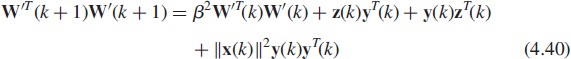
with ![]() , which implies (see Exercise 4.9) the following recursions
, which implies (see Exercise 4.9) the following recursions
![]()
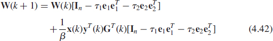
where τ1, τ2 and e1, e2 are defined in Exercise 4.9.
Note that the square root inverse matrix G(k + 1) of ![]() is asymmetric even if G(0) is symmetric. Expressions (4.41) and (4.42) provide an algorithm which does not involve any matrix–matrix multiplications and in fact requires only O(nr) operations.
is asymmetric even if G(0) is symmetric. Expressions (4.41) and (4.42) provide an algorithm which does not involve any matrix–matrix multiplications and in fact requires only O(nr) operations.
Based on the approximation that W(k) and W(k + 1) span the same r-dimensional subspace, another power-based algorithm referred to as the approximated power iteration (API) algorithm and its fast implementation (FAPI) have been proposed in [8]. Compared to the NP3 algorithm, this scheme has the advantage that it can handle the exponential (4.19) or the sliding windowed (4.22) estimates of Cx(k) in the same framework (and with the same complexity of O(nr) operations) by writing (4.19) and (4.22) in the form
![]()
with J = 1 and x′(k) = x(k) for the exponential window and ![]() and x′(k) = [x(k), x(k − l)] for the sliding window [see (4.22)]. Among the power-based minor subspace tracking methods issued from the exponential of sliding window, this FAPI algorithm has been considered by many practitioners (e.g. [11]) as outperforming the other algorithms having the same computational complexity.
and x′(k) = [x(k), x(k − l)] for the sliding window [see (4.22)]. Among the power-based minor subspace tracking methods issued from the exponential of sliding window, this FAPI algorithm has been considered by many practitioners (e.g. [11]) as outperforming the other algorithms having the same computational complexity.
4.5.2 Projection Approximation-based Methods
Since (4.14) describes an unconstrained cost function to be minimized, it is straightforward to apply the gradient-descent technique for dominant subspace tracking. Using expression (4.90) of the gradient given in Exercise 4.7 with the estimate x(k)xT(k) of Cx(k) gives

We note that this algorithm can be linked to Oja's algorithm (4.30). First, the term between brackets is the symmetrization of the term −x(k)xT(k) + W(k)WT(k)x(k)xT(k) of Oja's algorithm (4.30). Second, we see that when WT(k)W(k) is approximated by Ir (which is justified from the stability property below), algorithm (4.43) gives Oja's algorithm (4.30). We note that because the field of the stochastic approximation algorithm (4.43) is the opposite of the derivative of the positive function (4.14), the orthonormal bases of the dominant subspace are globally asymptotically stable for its associated ODE (see Subsection 4.7.1) in contrast to Oja's algorithm (4.30), for which they are only locally asymptotically stable. A complete performance analysis of the stochastic approximation algorithm (4.43) has been presented in [24] where closed-form expressions of the asymptotic covariance of the estimated projection matrix W(k)WT(k) are given and commented on for independent Gaussian data x(k) and constant stepsize μ.
If now Cx(k) is estimated by the exponentially weighted sample covariance matrix ![]() (4.18) instead of x(k)xT(k), the scalar function J(W) becomes
(4.18) instead of x(k)xT(k), the scalar function J(W) becomes
and all data x(i) available in the time interval {0, …, k} are involved in estimating the dominant subspace at time instant k + 1 supposing this estimate is known at time instant k. The key issue of the projection approximation subspace tracking algorithm (PAST) proposed by Yang in [71] is to approximate WT(k)x(i) in (4.44), the unknown projection of x(i) onto the columns of W(k) by the expression y(i) = WT(i)x(i) which can be calculated for all 0 ≤ i ≤ k at the time instant k. This results in the following modified cost function
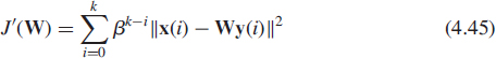
which is now quadratic in the elements of W. This projection approximation, hence the name PAST, changes the error performance surface of J(W). For stationary or slowly varying Cx(k), the difference between WT(k)x(i) and WT(i)x(i) is small, in particular when i is close to k. However, this difference may be larger in the distant past with i « k, but the contribution of the past data to the cost function (4.45) is decreasing for growing k, due to the exponential windowing. It is therefore expected that J′(W) will be a good approximation to J(W) and the matrix W(k) minimizing J′(W) be a good estimate for the dominant subspace of Cx(k). In case of sudden parameter changes of the model (4.15), the numerical experiments presented in [71] show that the algorithms derived from the PAST approach still converge. The main advantage of this scheme is that the least square minimization of (4.45) whose solution is given by ![]() where
where ![]() and
and ![]() has been extensively studied in adaptive filtering (see e.g. [36, Chap. 13] and [68, Chap. 12]) where various recursive least square algorithms (RLS) based on the matrix inversion lemma have been proposed.7 We note that because of the approximation of J(W) by J′(W), the columns of W(k) are not exactly orthonormal. But this lack of orthonormality does not mean that we need to perform a reorthonormalization of W(k) after each update. For this algorithm, the necessity of orthonormalization depends solely on the post processing method which uses this signal subspace estimate to extract the desired signal information (see e.g. Section 4.8). It is shown in the numerical experiments presented in [71] that the deviation of W(k) from orthonormality is very small and for a growing sliding window (β = 1), W(k) converges to a matrix with exactly orthonormal columns under stationary signal. Finally, note that a theoretical study of convergence and a derivation of the asymptotic distribution of the recursive subspace estimators have been presented in [73, 74] respectively. Using the ODE associated with this algorithm (see Section 4.7.1) which is here a pair of coupled matrix differential equations, it is proved that under signal stationarity and other weak conditions, the PAST algorithm converges to the desired signal subspace with probability one.
has been extensively studied in adaptive filtering (see e.g. [36, Chap. 13] and [68, Chap. 12]) where various recursive least square algorithms (RLS) based on the matrix inversion lemma have been proposed.7 We note that because of the approximation of J(W) by J′(W), the columns of W(k) are not exactly orthonormal. But this lack of orthonormality does not mean that we need to perform a reorthonormalization of W(k) after each update. For this algorithm, the necessity of orthonormalization depends solely on the post processing method which uses this signal subspace estimate to extract the desired signal information (see e.g. Section 4.8). It is shown in the numerical experiments presented in [71] that the deviation of W(k) from orthonormality is very small and for a growing sliding window (β = 1), W(k) converges to a matrix with exactly orthonormal columns under stationary signal. Finally, note that a theoretical study of convergence and a derivation of the asymptotic distribution of the recursive subspace estimators have been presented in [73, 74] respectively. Using the ODE associated with this algorithm (see Section 4.7.1) which is here a pair of coupled matrix differential equations, it is proved that under signal stationarity and other weak conditions, the PAST algorithm converges to the desired signal subspace with probability one.
To speed up the convergence of the PAST algorithm and to guarantee the orthonormality of W(k) at each iteration, an orthonormal version of the PAST algorithm dubbed OPAST has been proposed in [1]. This algorithm consists of the PAST algorithm where W(k + 1) is related to W(k) by W(k + 1) = W(k) + p(k)q(k), plus an orthonormalization step of W(k) based on the same approach as those used in the FRANS algorithm (see Subsection 4.5.1) which leads to the update W(k + 1) = W(k) + p′(k)q(k).
Note that the PAST algorithm cannot be used to estimate the noise subspace by simply changing the sign of the stepsize because the associated ODE is unstable. Efforts to eliminate this instability were attempted in [4] by forcing the orthonormality of W(k) at each time step. Although there was a definite improvement in the stability characteristics, the resulting algorithm remains numerically unstable.
4.5.3 Additional Methodologies
Various generalizations of criteria (4.7) and (4.14) have been proposed (e.g. in [41]), which generally yield robust estimates of principal subspaces or eigenvectors that are totally different from the standard ones. Among them, the following novel information criterion (NIC) [48] results in a fast algorithm to estimate the principal subspace with a number of attractive properties
![]()
given that W lies in the domain {W such that WTCW > 0}, where the matrix logarithm is defined, for example, in [35, Chap. 11]. It is proved in [48] (see also Exercises 4.11 and 4.12) that the above criterion has a global maximum that is attained when and only when W = UrQ where Ur = [u1, …, ur] and Q is an arbitrary r × r orthogonal matrix and all the other stationary points are saddle points. Taking the gradient of (4.46) [which is given explicitly by (4.92)], the following gradient ascent algorithm has been proposed in [48] for updating the estimate W(k)
![]()
Using the recursive estimate ![]() (4.18), and the projection approximation introduced in [71] WT(k)x(i) = WT(i)x(i) for all 0 ≤ i ≤ k, the update (4.47) becomes
(4.18), and the projection approximation introduced in [71] WT(k)x(i) = WT(i)x(i) for all 0 ≤ i ≤ k, the update (4.47) becomes

with ![]() . Consequently, similarly to the PAST algorithms, standard RLS techniques used in adaptive filtering can be applied. According to the numerical experiments presented in [38], this algorithm performs very similarly to the PAST algorithm also having the same complexity. Finally, we note that it has been proved in [48] that the points W = UrQ are the only asymptotically stable points of the ODE (see Subsection 4.7.1) associated with the gradient ascent algorithm (4.47) and that the attraction set of these points is the domain {W such that WTCW > 0}. But to the best of our knowledge, no complete theoretical performance analysis of algorithm (4.48) has been carried out so far.
. Consequently, similarly to the PAST algorithms, standard RLS techniques used in adaptive filtering can be applied. According to the numerical experiments presented in [38], this algorithm performs very similarly to the PAST algorithm also having the same complexity. Finally, we note that it has been proved in [48] that the points W = UrQ are the only asymptotically stable points of the ODE (see Subsection 4.7.1) associated with the gradient ascent algorithm (4.47) and that the attraction set of these points is the domain {W such that WTCW > 0}. But to the best of our knowledge, no complete theoretical performance analysis of algorithm (4.48) has been carried out so far.
4.6 EIGENVECTORS TRACKING
Although, the adaptive estimation of the dominant or minor subspace through the estimate W(k)WT(k) of the associated projector is of most importance for subspace-based algorithms, there are situations where the associated eigenvalues are simple (λ1 > … > λr > λr+1 or λn < … < λn−r+1 < λn−r) and the desired estimated orthonormal basis of this space must form an eigenbasis. This is the case for the statistical technique of principal component analysis in data compression and coding, optimal feature extraction in pattern recognition, and for optimal fitting in the total least square sense, or for Karhunen-Loève transformation of signals, to mention only a few examples. In these applications, {y1(k), …, yr(k)} or {yn(k), …, yn−r+1(k)} with ![]() where W = [w1(k), …, wr(k)] or W = [wn(k), …, wn−r+1(k)] are the estimated r first principal or r last minor components of the data x(k). To derive such adaptive estimates, the stochastic approximation algorithms that have been proposed, are issued from adaptations of the iterative constrained maximizations (4.5) and minimizations (4.6) of Rayleigh quotients; the weighted subspace criterion (4.8); the orthogonal iterations (4.11) and, finally the gradient-descent technique applied to the minimization of (4.14).
where W = [w1(k), …, wr(k)] or W = [wn(k), …, wn−r+1(k)] are the estimated r first principal or r last minor components of the data x(k). To derive such adaptive estimates, the stochastic approximation algorithms that have been proposed, are issued from adaptations of the iterative constrained maximizations (4.5) and minimizations (4.6) of Rayleigh quotients; the weighted subspace criterion (4.8); the orthogonal iterations (4.11) and, finally the gradient-descent technique applied to the minimization of (4.14).
4.6.1 Rayleigh Quotient-based Methods
To adapt maximization (4.5) and minimization (4.6) of Rayleigh quotients to adaptive implementations, a method has been proposed in [61]. It is derived from a Givens parametrization of the constraint WTW = Ir, and from a gradient-like procedure. The Givens rotations approach introduced by Regalia [61] is based on the properties that any n × 1 unit 2-norm vector and any orthogonal vector to this vector can be respectively written as the last column of an n × n orthogonal matrix and as a linear combination of the first n − 1 columns of this orthogonal matrix, that is,
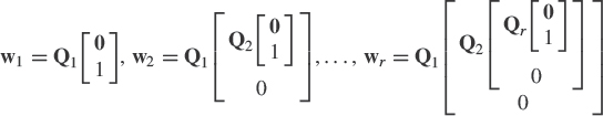
where Qi is the following orthogonal matrix of order n − i + 1
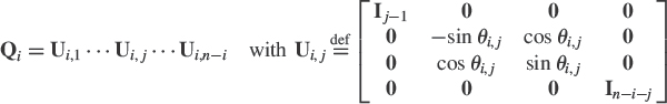
and θi,j belongs to ![]() . The existence of such a parametrization8 for all orthonormal sets {w1, …, wr} is proved in [61]. It consists of r(2n − r − 1)/2 real parameters. Furthermore, this parametrization is unique if we add some constraints on θi,j. A deflation procedure, inspired by the maximization (4.5) and minimization (4.6) has been proposed [61]. First the maximization or minimization (4.3) is performed with the help of the classical stochastic gradient algorithm, in which the parameters are θ1,1, …, θ1,n−1, whereas the maximization (4.5) or minimization (4.6) are realized thanks to stochastic gradient algorithms with respect to the parameters θi,1, …, θi,n−i, in which the preceding parameters θl,1(k), …, θl,n−l(k) for l = 1, …, i − 1 are injected from the i − 1 previous algorithms. The deflation procedure is achieved by coupled stochastic gradient algorithms
. The existence of such a parametrization8 for all orthonormal sets {w1, …, wr} is proved in [61]. It consists of r(2n − r − 1)/2 real parameters. Furthermore, this parametrization is unique if we add some constraints on θi,j. A deflation procedure, inspired by the maximization (4.5) and minimization (4.6) has been proposed [61]. First the maximization or minimization (4.3) is performed with the help of the classical stochastic gradient algorithm, in which the parameters are θ1,1, …, θ1,n−1, whereas the maximization (4.5) or minimization (4.6) are realized thanks to stochastic gradient algorithms with respect to the parameters θi,1, …, θi,n−i, in which the preceding parameters θl,1(k), …, θl,n−l(k) for l = 1, …, i − 1 are injected from the i − 1 previous algorithms. The deflation procedure is achieved by coupled stochastic gradient algorithms
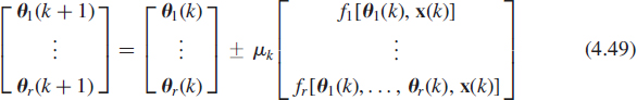
with ![]() and
and ![]() . This rather intuitive computational process was confirmed by simulation results [61]. Later a formal analysis of the convergence and performance was performed in [23] where it has been proved that the stationary points of the associated ODE are globally asymptotically stable (see Subsection 4.7.1) and that the stochastic algorithm (4.49) converges almost surely to these points for stationary data x(k) when μk is decreasing with
. This rather intuitive computational process was confirmed by simulation results [61]. Later a formal analysis of the convergence and performance was performed in [23] where it has been proved that the stationary points of the associated ODE are globally asymptotically stable (see Subsection 4.7.1) and that the stochastic algorithm (4.49) converges almost surely to these points for stationary data x(k) when μk is decreasing with ![]() = and
= and ![]() . We note that this algorithm yields exactly orthonormal r dominant or minor estimated eigenvectors by a simple change of sign in its stepsize, and requires O(nr) operations at each iteration but without accounting for the trigonometric functions.
. We note that this algorithm yields exactly orthonormal r dominant or minor estimated eigenvectors by a simple change of sign in its stepsize, and requires O(nr) operations at each iteration but without accounting for the trigonometric functions.
Alternatively, a stochastic gradient-like algorithm denoted direct adaptive subspace estimation (DASE) has been proposed in [62] with a direct parametrization of the eigenvectors by means of their coefficients. Maximization or minimization (4.3) is performed with the help of a modification of the classic stochastic gradient algorithm to assure an approximate unit norm of the first estimated eigenvector w1(k) [in fact a rewriting of Oja's neuron (4.23)]. Then, a modification of the classical stochastic gradient algorithm using a deflation procedure, inspired by the constraint WTW = Ir gives the estimates [wi(k)]i=2, …, r

This totally empirical procedure has been studied in [63]. It has been proved that the stationary points of the associated ODE are all eigenvector bases {±ui1, …, ±uir}. Using the eigenvalues of the derivative of the mean field (see Subsection 4.7.1), it is shown that all these eigenvector bases are unstable except {±u1} for r = 1 associated with the sign + [where algorithm (4.50) is Oja's neuron (4.23)]. But a closer, examination of these eigenvalues that are all real-valued, shows that for only the eigenbasis {±u1, …, ±ur} and {±un, …, ±un−r+1} associated with the sign + and − respectively, all the eigenvalues of the derivative of the mean field are strictly negative except for the eigenvalues associated with variations of the eigenvectors {±u1, …, ±ur} and {±un, …, ±un−r+1} in their directions. Consequently, it is claimed in [63] that if the norm of each estimated eigenvector is set to one at each iteration, the stability of the algorithm is ensured. The simulations presented in [62] confirm this intuition.
4.6.2 Eigenvector Power-based Methods
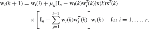
Note that similarly to the subspace criterion (4.7), the maximization or minimization of the weighted subspace criterion (4.8) ![]() subject to the constraint WTW = Ir can be solved by a constrained gradient-descent technique. Clearly, the simplest selection for C(k) is the instantaneous estimate x(k)xT(k). Because in this case, ∇WJ = 2x(k)xT(k)WΩ, we obtain the following stochastic approximation algorithm that will be a starting point for a family of algorithms that have been derived to adaptively estimate major or minor eigenvectors
subject to the constraint WTW = Ir can be solved by a constrained gradient-descent technique. Clearly, the simplest selection for C(k) is the instantaneous estimate x(k)xT(k). Because in this case, ∇WJ = 2x(k)xT(k)WΩ, we obtain the following stochastic approximation algorithm that will be a starting point for a family of algorithms that have been derived to adaptively estimate major or minor eigenvectors
![]()
in which W(k) = [w1(k), …, wr(k)] and the matrix Ω is a diagonal matrix Diag(ω1, …, ωr) with ω1 > … > ωr > 0. G(k + 1) is a matrix depending on
![]()
which orthonormalizes or approximately orthonormalizes the columns of W′(k + 1). Thus, W(k) has orthonormal or approximately orthonormal columns for all k. Depending on the form of matrix G(k + 1), variants of the basic stochastic algorithm are obtained. Going back to the general expression (4.29) of the subspace power-based algorithm, we note that (4.51) can also be derived from (4.29), where different stepsizes μkω1,…, μkωr are introduced for each column of W(k).
Using the same approach as for deriving (4.30), that is, where G(k + 1) is the symmetric square root inverse of ![]() , we obtain the following stochastic approximation algorithm
, we obtain the following stochastic approximation algorithm

Note that in contrast to the Oja's algorithm (4.30), this algorithm is different from the algorithm issued from the optimization of the cost function ![]() defined on the set of n × r orthogonal matrices W with the help of continuous-time matrix algorithms (see e.g. [21, Ch. 7.2], [19, Ch. 4] or (4.91) in Exercise 4.15).
defined on the set of n × r orthogonal matrices W with the help of continuous-time matrix algorithms (see e.g. [21, Ch. 7.2], [19, Ch. 4] or (4.91) in Exercise 4.15).
![]()
We note that these two algorithms reduce to the Oja's algorithm (4.30) for Ω = Ir and to Oja's neuron (4.23) for r = 1, which of course is unstable for tracking the minorant eigenvectors with the sign −. Techniques used for stabilizing Oja's algorithm (4.30) for minor subspace tracking, have been transposed to stabilize the weighted Oja's algorithm for tracking the minorant eigenvectors. For example, in [9], W(k) is forced to be orthonormal at each time step k as in [2] (see Exercise 4.10) with the MCA-OOja algorithm and the MCA-OOjaH algorithm using Householder transforms. Note, that by proving a recursion of the distance to orthonormality ![]() from a nonorthogonal matrix W(0), it has been shown in [10], that the latter algorithm is numerically stable in contrast to the former.
from a nonorthogonal matrix W(0), it has been shown in [10], that the latter algorithm is numerically stable in contrast to the former.
Instead of deriving a stochastic approximation algorithm from a specific orthonormalization matrix G(k + 1), an analogy with Oja's algorithm (4.30) has been used in [54] to derive the following algorithm

It has been proved in [55], that for tracking the dominant eigenvectors (i.e. with the sign +), the eigenvectors {±u1, …,±ur} are the only locally asymptotically stable points of the ODE associated with (4.54). But to the best of our knowledge, no complete theoretical performance analysis of these three algorithms (4.52), (4.53), and (4.54), has been carried out until now, except in [27] which gives the asymptotic distribution of the estimated principal eigenvectors.
If now the matrix G(k + 1) performs the Gram–Schmidt orthonormalization on the columns of W′(k + 1), an algorithm, denoted stochastic gradient ascent (SGA) algorithm, is obtained if the successive columns of matrix W(k + 1) are expanded, assuming μk is sufficiently small. By omitting the ![]() term in this expansion [51], we obtain the following algorithm
term in this expansion [51], we obtain the following algorithm

where here Ω = Diag(α1, α2, …, αr) with αi arbitrary strictly positive numbers.
The so called generalized Hebbian algorithm (GHA) is derived from Oja's algorithm (4.30) by replacing the matrix WT(k)x(k)xT(k)W(k) of Oja's algorithm by its diagonal and superdiagonal only
![]()
in which the operator upper sets all subdiagonal elements of a matrix to zero. When written columnwise, this algorithm is similar to the SGA algorithm (4.57) where αi = 1, i = 1, …, r, with the difference that there is no coefficient 2 in the sum

Oja et al. [54] proposed an algorithm denoted weighted subspace algorithm (WSA), which is similar to the Oja's algorithm, except for the scalar parameters β1, …, βr
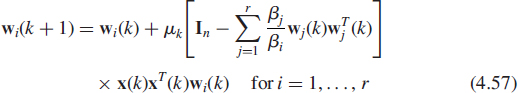
with β1 > … > βr > 0. If βi = 1 for all i, this algorithm reduces to Oja's algorithm.
Following the deflation technique introduced in the adaptive principal component extraction (APEX) algorithm [42], note finally that Oja's neuron can be directly adapted to estimate the r principal eigenvectors by replacing the instantaneous estimate x(k)xT(k) of Cx(k) by ![]() to successively estimate wi(k), i = 2, …, r
to successively estimate wi(k), i = 2, …, r
Minor component analysis was also considered in neural networks to solve the problem of optimal fitting in the total least square sense. Xu et al. [79] introduced the optimal fitting analyzer (OFA) algorithm by modifying the SGA algorithm. For the estimate wn(k) of the eigenvector associated with the smallest eigenvalue, this algorithm is derived from the Oja's neuron (4.23) by replacing x(k)xT(k) by In−x(k)xT(k), viz
![]()
and for i = n, …, n − r + 1, his algorithm reads
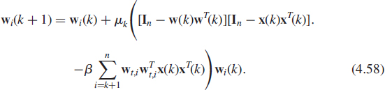
Oja [53] showed that, under the conditions that the eigenvalues are distinct, and that λn−r+1 < 1 and ![]() , the only asymptotically stable points of the associated ODE are the eigenvectors {±vn, …, ±vn−r+1}. Note that the magnitude of the eigenvalues must be controlled in practice by normalizing x(k) so that the expression between brackets in (4.58) becomes homogeneous.
, the only asymptotically stable points of the associated ODE are the eigenvectors {±vn, …, ±vn−r+1}. Note that the magnitude of the eigenvalues must be controlled in practice by normalizing x(k) so that the expression between brackets in (4.58) becomes homogeneous.
The derivation of these algorithms seems empirical. In fact, they have been derived from slight modifications of the ODE (4.75) associated with the Oja's neuron in order to keep adequate conditions of stability (see e.g. [53]). It was established by Oja [52], Sanger [67], and Oja et al. [55] for the SGA, GHA, and WSA algorithms respectively, that the only asymptotically stable points of their associated ODE are the eigenvectors {±v1, …, ±vr}. We note that the first vector (k = 1) estimated by the SGA and GHA algorithms, and the vector (r = k = 1) estimated by the SNL and WSA algorithms gives the constrained Hebbian learning rule of the basic PCA neuron (4.23) introduced by Oja [50].
A performance analysis of different eigenvector power-based algorithms has been presented in [22]. In particular, the asymptotic distribution of the eigenvector estimates and of the associated projection matrices given by these stochastic algorithms with constant stepsize μ for stationary data has been derived, where closed-form expressions of the covariance of these distributions has been given and analyzed for independent Gaussian distributed data x(k). Closed-form expressions of the mean square error of these estimators has been deduced and analyzed. In particular, they allow us to specify the influence of the different parameters (α2, …, αr), (β1, …, βr) and β of these algorithms on their performance and to take into account tradeoffs between the misadjustment and the speed of convergence. An example of such derivation and analysis is given for the Oja's neuron in Subsection 4.7.3.
Eigenvector Power-based Methods Issued from Exponential Windows Using the exponential windowed estimates (4.19) of Cx(k), and following the concept of power method (4.9) and the subspace deflation technique introduced in [42], the following algorithm has been proposed in [38]
![]()
![]()
where ![]() for i = 1, …, r. Applying the approximation
for i = 1, …, r. Applying the approximation ![]() in (4.59) to reduce the complexity, (4.59) becomes
in (4.59) to reduce the complexity, (4.59) becomes
![]()
with ![]() and
and ![]() . Equations (4.61) and (4.59) should be run successively for i = 1, …, r at each iteration k.
. Equations (4.61) and (4.59) should be run successively for i = 1, …, r at each iteration k.
Note that up to a common factor estimate of the eigenvalues λi(k + 1) of Cx(k) can be updated as follows. From (4.59), one can write
![]()
Using (4.61) and applying the approximations ![]() and ci(k) ≈ 0, one can replace (4.62) by
and ci(k) ≈ 0, one can replace (4.62) by
![]()
that can be used to track the rank r and the signal eigenvectors, as in [72].
4.6.3 Projection Approximation-based Methods
A variant of the PAST algorithm, named PASTd and presented in [71], allows one to estimate the r dominant eigenvectors. This algorithm is based on a deflation technique that consists in estimating sequentially the eigenvectors. First the most dominant estimated eigenvector w1(k) is updated by applying the PAST algorithm with r = 1. Then the projection of the current data x(k) onto this estimated eigenvector is removed from x(k) itself. Because now the second dominant eigenvector becomes the most dominant one in the updated data vector ![]() , it can be extracted in the same way as before. Applying this procedure repeatedly, all of the r dominant eigenvectors and the associated eigenvalues are estimated sequentially. These estimated eigenvalues may be used to estimate the rank r if it is not known a priori [72]. It is interesting to note that for r = 1, the PAST and the PASTd algorithms, that are identical, simplify as
, it can be extracted in the same way as before. Applying this procedure repeatedly, all of the r dominant eigenvectors and the associated eigenvalues are estimated sequentially. These estimated eigenvalues may be used to estimate the rank r if it is not known a priori [72]. It is interesting to note that for r = 1, the PAST and the PASTd algorithms, that are identical, simplify as
![]()
where ![]() with
with ![]() and
and ![]() . A comparison with Oja's neuron (4.23) shows that both algorithms are identical except for the stepsize. While Oja's neuron uses a fixed stepsize μ which needs careful tuning, (4.63) implies a time varying, self-tuning stepsize μk. The numerical experiments presented in [71] show that this deflation procedure causes a stronger loss of orthonormality between wi(k) and a slight increase in the error in the successive estimates wi(k). By invoking the ODE approach (see Section 4.7.1), it has been proved in [73] for stationary signals and other weak conditions, that the PASTd algorithm converges to the desired r dominant eigenvectors with probability one.
. A comparison with Oja's neuron (4.23) shows that both algorithms are identical except for the stepsize. While Oja's neuron uses a fixed stepsize μ which needs careful tuning, (4.63) implies a time varying, self-tuning stepsize μk. The numerical experiments presented in [71] show that this deflation procedure causes a stronger loss of orthonormality between wi(k) and a slight increase in the error in the successive estimates wi(k). By invoking the ODE approach (see Section 4.7.1), it has been proved in [73] for stationary signals and other weak conditions, that the PASTd algorithm converges to the desired r dominant eigenvectors with probability one.
In contrast to the PAST algorithm, the PASTd algorithm can be used to estimate the minor eigenvectors by changing the sign of the stepsize with an orthonormalization of the estimated eigenvectors at each step. It has been proved [65] that for β = 1, the only locally asymptotically stable points of the associated ODE are the desired eigenvectors {±vn, …, ±vn−r+1}. To reduce the complexity of the Gram–Schmidt orthonormalization step used in [65], [9] proposed a modification of this part.
4.6.4 Additional Methodologies
Among the other approaches to adaptively estimate the eigenvectors of a covariance matrix, the maximum likelihood adaptive subspace estimation (MALASE) [18] provides a number of desirable features. It is based on the adaptive maximization of the log-likelihood of the EVD parameters associated with the covariance matrix Cx for Gaussian distributed zero-mean data x(k). Up to an additive constant, this log-likelihood is given by
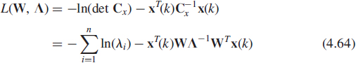
where Cx = WΛWT represents the EVD of Cx with W an orthogonal n × n matrix and Λ = Diag(λ1, …, λn). This is a quite natural criterion for statistical estimation purposes, even if the minimum variance property of the likelihood functional is actually an asymptotic property. To deduce an adaptive algorithm, a gradient ascent procedure has been proposed in [18] in which a new data x(k) is used at each time iteration k of the maximization of (4.64). Using the differential of L(W, Λ) defined on the manifold of n × n orthogonal matrices [see [21, pp. 62–63] or Exercise 4.15 (4.93)], we obtain the following gradient of L(W, Λ)
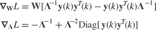
where ![]() . Then, the stochastic gradient update of W yields
. Then, the stochastic gradient update of W yields
![]()
![]()
where the stepsizes μk and ![]() are possibly different. We note that, starting from an orthonormal matrix W(0), the sequence of estimates W(k) given by (4.65) is orthonormal up to the second-order term in μk only. To ensure in practice the convergence of this algorithm, is has been shown in [18] that it is necessary to orthonormalize W(k) quite often to compensate for the orthonormality drift in
are possibly different. We note that, starting from an orthonormal matrix W(0), the sequence of estimates W(k) given by (4.65) is orthonormal up to the second-order term in μk only. To ensure in practice the convergence of this algorithm, is has been shown in [18] that it is necessary to orthonormalize W(k) quite often to compensate for the orthonormality drift in ![]() . Using continuous-time system theory and differential geometry [21], a modification of (4.65) has been proposed in [18]. It is clear that ∇WL is tangent to the curve defined by
. Using continuous-time system theory and differential geometry [21], a modification of (4.65) has been proposed in [18]. It is clear that ∇WL is tangent to the curve defined by
![]()
for t = 0, where the matrix exponential is defined, for example, in [35, Chap. 11]. Furthermore, we note that this curve lies in the manifold of orthogonal matrices if W(0) is orthogonal because exp(A) is orthogonal if and only if A is skew-symmetric (AT = −A) and matrix Λ−1y(k)yT(k) − y(k)yT(k)Λ−1 is clearly skew-symmetric. Moving on the curve W(t) from point t = 0 in the direction of increasing values of ∇WL amounts to letting t increase. Thus, a discretized version of the optimization of L(W, Λ) as a continuous function of W is given by the following update scheme
![]()
and the coupled update equations (4.66) and (4.67) form the MALASE algorithm. As mentioned above the update factor ![]() is an orthogonal matrix. This ensures that the orthonormality property is preserved by the MALASE algorithm, provided that the algorithm is initialized with an orthogonal matrix W(0). However, it has been shown by the numerical experiments presented in [18], that it is not necessary to have W(0) orthogonal to ensure the convergence, since the MALASE algorithm steers W(k) towards the manifold of orthogonal matrices. The MALASE algorithm seems to involve high computational cost, due to the matrix exponential that applies in (4.67). However, since
is an orthogonal matrix. This ensures that the orthonormality property is preserved by the MALASE algorithm, provided that the algorithm is initialized with an orthogonal matrix W(0). However, it has been shown by the numerical experiments presented in [18], that it is not necessary to have W(0) orthogonal to ensure the convergence, since the MALASE algorithm steers W(k) towards the manifold of orthogonal matrices. The MALASE algorithm seems to involve high computational cost, due to the matrix exponential that applies in (4.67). However, since ![]() is the exponential of a sum of two rank-one matrices, the calculation of this matrix requires only O(n2) operations [18]. Originally, this algorithm which updates the EVD of the covariance matrix Cx(k) can be modified by a simple preprocessing to estimate the principal or minor r signal eigenvectors only, when the remaining n − r eigenvectors are associated with a common eigenvalue σ2(k) (see Subsection 4.3.1). This algorithm, denoted MALASE(r) requires O(nr) operations by iteration. Finally, note that a theoretical analysis of convergence has been presented in [18]. It is proved that in stationary environments, the stationary stable points of the algorithm (4.66), (4.67) correspond to the EVD of Cx. Furthermore, the covariance of the asymptotic distribution of the estimated parameters is given for Gaussian independently distributed data x(k) using general results of Gaussian approximation (see Subsection 4.7.2).
is the exponential of a sum of two rank-one matrices, the calculation of this matrix requires only O(n2) operations [18]. Originally, this algorithm which updates the EVD of the covariance matrix Cx(k) can be modified by a simple preprocessing to estimate the principal or minor r signal eigenvectors only, when the remaining n − r eigenvectors are associated with a common eigenvalue σ2(k) (see Subsection 4.3.1). This algorithm, denoted MALASE(r) requires O(nr) operations by iteration. Finally, note that a theoretical analysis of convergence has been presented in [18]. It is proved that in stationary environments, the stationary stable points of the algorithm (4.66), (4.67) correspond to the EVD of Cx. Furthermore, the covariance of the asymptotic distribution of the estimated parameters is given for Gaussian independently distributed data x(k) using general results of Gaussian approximation (see Subsection 4.7.2).
4.6.5 Particular Case of Second-order Stationary Data
Finally, note that for x(k) = [x(k), x(k − 1), …, x(k − n + 1)]T comprising of time delayed versions of scalar valued second-order stationary data x(k), the covariance matrix Cx(k) = E[x(k)xT(k)] is Toeplitz and consequently centro-symmetric. This property occurs in important applications—temporal covariance matrices obtained from a uniform sampling of a second-order stationary signals, and spatial covariance matrices issued from uncorrelated and band-limited sources observed on a centro-symmetric sensor array (e.g. on uniform linear arrays). This centro-symmetric structure of Cx allows us to use for real-valued data, the property9 [14] that its EVD can be obtained from two orthonormal eigenbases of half-size real symmetric matrices. For example if n is even, Cx can be partitioned as follows
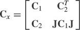
where J is a n/2 × n/2 matrix with ones on its antidiagonal and zeroes elsewhere. Then, the n unit 2-norm eigenvectors vi of Cx are given by n/2 symmetric and n/2 skew symmetric vectors ![]() where εi = ±1, respectively issued from the unit 2-norm eigenvectors ui of
where εi = ±1, respectively issued from the unit 2-norm eigenvectors ui of ![]() with
with ![]() . This property has been exploited [23, 26] to reduce the computational cost of the previously introduced eigenvectors adaptive algorithms. Furthermore, the conditioning of these two independent EVDs is improved with respect to the EVD of Cx since the difference between the two consecutive eigenvalues increases in general. Compared to the estimators that do not take the centro-symmetric structure into account, the performance ought to be improved. This has been proved in [26], using closed-form expressions of the asymptotic bias and covariance of eigenvectors power-based estimators with constant stepsize μ derived in [22] for independent Gaussian distributed data x(k). Finally, note that the deviation from orthonormality is reduced and the convergence speed is improved, yielding a better tradeoff between convergence speed and misadjustment.
. This property has been exploited [23, 26] to reduce the computational cost of the previously introduced eigenvectors adaptive algorithms. Furthermore, the conditioning of these two independent EVDs is improved with respect to the EVD of Cx since the difference between the two consecutive eigenvalues increases in general. Compared to the estimators that do not take the centro-symmetric structure into account, the performance ought to be improved. This has been proved in [26], using closed-form expressions of the asymptotic bias and covariance of eigenvectors power-based estimators with constant stepsize μ derived in [22] for independent Gaussian distributed data x(k). Finally, note that the deviation from orthonormality is reduced and the convergence speed is improved, yielding a better tradeoff between convergence speed and misadjustment.
4.7 CONVERGENCE AND PERFORMANCE ANALYSIS ISSUES
Several tools may be used to assess the convergence and the performance of the previously described algorithms. First of all, note that despite the simplicity of the LMS algorithm (see e.g. [36])
![]()
its convergence and associated analysis has been the subject of many contributions in the past three decades (see e.g. [68] and references therein). However, in-depth theoretical studies are still a matter of utmost interest. Consequently, due to their complexity with respect to the LMS algorithm, results about the convergence and performance analysis of subspaces or eigenvectors tracking will be much weaker.
To study the convergence of the algorithms introduced in the previous two sections from a theoretical point of view, the data x(k) will be supposed to be stationary and the stepsize μk will be considered as decreasing. In these conditions, according to the addressed problem, some questions arise. Does the sequence W(k)WT(k) converge almost surely to the signal Πs or the noise projector Πn? And does the sequence WT(k)W(k) converge almost surely to Ir for the subspace tracking problem? Or does the sequence W(k) converge to the signal or the noise eigenvectors [±u1, …, ±ur] or [±un−r+1, …, ±un] for the eigenvectors tracking problems? These questions are very challenging, but using the stability of the associated ODE, a partial response will be given in Subsection 4.7.1.
Now, from a practical point of view, the stepsize sequence μk is reduced to a small constant μ to track signal or noise subspaces (or signal or noise eigenvectors) with possible nonstationary data x(k). Under these conditions, the previous sequences do not converge almost surely any longer even for stationary data x(k). Nevertheless, if for stationary data, these algorithms converge almost surely with a decreasing stepsize, their estimate θ(k) (W(k)WT(k), WT(k)W(k) or W(k) according to the problem) will oscillate around their limit θ* (Πs or Πn, Ir, [±u1, …, ±ur] or [±un−r+1, …, ±un], according to the problem) with a constant small step size. In these later conditions, the performance of the algorithms will be assessed by the covariance matrix of the errors [θ(k) − θ*] using some results of Gaussian approximation recalled in Subsection 4.7.2.
Unfortunately, the study of the stability of the associated ODE and the derivation of the covariance of the errors are not always possible due to their complex forms. In these cases, the convergence and the performance of the algorithms for stationary data will be assessed by first-order analysis using coarse approximations. In practice, this analysis will be possible only for independent data x(k) and assuming the stepsize μ is sufficiently small to keep terms that are at most of the order of μ in the different used expansions. An example of such analysis has been used in [30, 75] to derive an approximate expression of the mean of the deviation from orthonormality E[WT(k)W(k) − Ir] for the estimate W(k) given by the FRANS algorithm (described in Subsection 4.5.1) that allows to explain the difference in behavior of this algorithm when estimating the noise and signal subspaces.
4.7.1 A Short Review of the ODE Method
The so-called ODE [13, 43] is a powerful tool to study the asymptotic behavior of the stochastic approximation algorithms of the general form10
![]()
with x(k) = g[ξ(k)], where ξ(k) is a Markov chain that does not depend on θ, f(θ, x) and h(θ, x) are regular enough functions, and where ![]() is a positive sequence of constants, converging to zero, and satisfying the assumption
is a positive sequence of constants, converging to zero, and satisfying the assumption ![]() . Then, the convergence properties of the discrete time stochastic algorithm (4.68) is intimately connected to the stability properties of the deterministic ODE associated with (4.68), which is defined as the first-order ordinary differential equation
. Then, the convergence properties of the discrete time stochastic algorithm (4.68) is intimately connected to the stability properties of the deterministic ODE associated with (4.68), which is defined as the first-order ordinary differential equation
![]()
where the function ![]() is defined by
is defined by
![]()
where the expectation is taken only with respect to the data x(k) and θ is assumed deterministic. We first recall in the following some definitions and results of stability theory of ODE (i.e., the asymptotic behavior of trajectories of the ODE) and then, we will specify its connection to the convergence of the stochastic algorithm (4.68). The stationary points of this ODE are the values θ* of θ for which the driving term ![]() vanishes; hence the term stationary ponts. This gives
vanishes; hence the term stationary ponts. This gives ![]() , so that the motion of the trajectory ceases. A stationary point θ* of the ODE is said to be
, so that the motion of the trajectory ceases. A stationary point θ* of the ODE is said to be
- stable if for an arbitrary neighborhood of θ*, the trajectory θ(t) stays in this neighborhood for an initial condition θ(0) in another neighborhood of θ*;
- locally asymptotically stable if there exists a neighborhood of θ* such that for all initial conditions θ(0) in this neighborhood, the ODE (4.69) forces θ(t) → θ* as t → ∞;
- globally asymptotically stable if for all possible values of initial conditions θ(0), the ODE (4.69) forces θ(t) → θ* as t → ∞;
- unstable if for all neighborhoods of θ*, there exists some initial value θ(0) in this neighborhood for which the ODE (4.69) do not force θ(t) to converge to θ* as t → ∞.
Assuming that the set of stationary points can be derived, two standard methods are used to test for stability. They are summarized in the following. The first consists in finding a Lyapunov function L(θ) for the differential equation (4.69), that is, a positive valued function that is decreasing along all trajectories. In this case, it is proved (see e.g. [12]) that the set of the stationary points θ* are asymptotically stable. This stability is local if this decrease occurs from an initial condition θ(0) located in a neighborhood of the stationary points and global if the initial condition can be arbitrary. If θ* is a (locally or globally) stable stationary point, then such a Lyapunov function necessarily exists [12]. But for general nonlinear functions ![]() , no general recipe exists for finding such a function. Instead, one must try many candidate Lyapunov functions in the hopes of uncovering one which works.
, no general recipe exists for finding such a function. Instead, one must try many candidate Lyapunov functions in the hopes of uncovering one which works.
However, for specific functions ![]() which constitute negative gradient vectors of a positive scalar function J(θ)
which constitute negative gradient vectors of a positive scalar function J(θ)
![]()
then, all the trajectories of the ODE (4.69) converge to the set of the stationary points of the ODE (see Exercise 4.16). Consequently, the set of the stationary points is globally asymptotically stable for this ODE.
The second method consists in a local linearization of the ODE (4.69) about each stationary point θ* in which case a stationary point is locally asymptotically stable if and only if the locally linearized equation is asymptotically stable. Consequently the final conclusion amounts to an eigenvalue check of the matrix ![]() . More precisely (see Exercise 4.17), if
. More precisely (see Exercise 4.17), if ![]() is a stationary point of the ODE (4.69), and ν1, …, νm are the eigenvalues of the m × m matrix
is a stationary point of the ODE (4.69), and ν1, …, νm are the eigenvalues of the m × m matrix ![]() , then (see Exercise 4.17 or [12] for a formal proof)
, then (see Exercise 4.17 or [12] for a formal proof)
- if all eigenvalues ν1, …, νm have strictly negative real parts, θ* is a locally asymptotically stable point;
- if there exists νi among ν1, …, νm such that
 is an unstable point;
 - if for all eigenvalues ν1, …, νm,
 and for at least one eigenvalue νi0 among ν1, …, νm,
  , we cannot conclude.
Considering now the connection between the stability properties of the associated deterministic ODE (4.69) and the convergence properties of the discrete time stochastic algorithm (4.68), several results are available. First, the sequence θ(k) generated by the algorithm (4.68) can only converge almost surely [13, 43] to a (locally or globally) asymptotically stable stationary point of the associated ODE (4.69). But deducing some convergence results about the stochastic algorithm (4.68) from the stability of the associated ODE is not trivial because a stochastic algorithm has much more complex asymptotic behavior than a given solution of its associated deterministic ODE. However under additional technical assumptions, it is proved [32] that if the ODE has a finite number of globally (up to a Lebesgue measure zero set of initial conditions) asymptotically stable stationary points (θ*i)i = 1,…, d and if each trajectory of the ODE converges towards one of theses points, then the sequence θ(k) generated by the algorithm (4.68) converges almost surely to one of these points. The conditions of the result are satisfied, in particular, if the mean field ![]() can be written as
can be written as ![]() where ∇θJ is a positive valued function admitting a finite number of local minima. In this later case, this result has been extended for an infinite number of isolated minima in [33].
where ∇θJ is a positive valued function admitting a finite number of local minima. In this later case, this result has been extended for an infinite number of isolated minima in [33].
In adaptive processing, we do not wish for a decreasing stepsize sequence, since we would then lose the tracking capability of the algorithms. To be able to track the possible nonstationarity of the data x(k), the sequence of stepsize is reduced to a small constant parameter μ. In this case, the stochastic algorithm (4.68) does not converge almost surely even for stationary data and the rigorous results concerning the asymptotic behavior of (4.68) are less powerful. However, when the set of all stable points (θ*i)i=1,…, d of the associated ODE (4.69) is globally asymptotically stable (up to a zero measure set of initial conditions), the weak convergence approach developed by Kushner [44] suggests that for a sufficiently small μ, θ(k) will oscillate around one of the limit points θ*i of the decreasing stepsize stochastic algorithm. In particular, one should note that, when there exists more than one possible limit (d ≠ 1), the algorithm may oscillate around one of them θ*i, and then move into a neighborhood of another equilibrium point θ*j. However, the probability of such events decreases to zero as μ → 0, so that their implication is marginal in most cases.
4.7.2 A Short Review of a General Gaussian Approximation Result
For constant stepsize algorithms and stationary data, we will use the following result proved in [13, Th. 2, p. 108] under a certain number of hypotheses. Consider the constant stepsize stochastic approximation algorithm (4.68). Suppose that θ(k) converges almost surely to the unique globally asymptotically stable point θ* in the corresponding decreasing stepsize algorithm. Then, if θμ(k) denotes the value of θ(k) associated with the algorithm of stepsize μ, we have when μ → 0 and k → ∞ (where ![]() denotes the convergence in distribution and
denotes the convergence in distribution and ![]() , the Gaussian distribution of mean m and covariance Cx)
, the Gaussian distribution of mean m and covariance Cx)
![]()
where Cθ is the unique solution of the continuous-time Lyapunov equation
![]()
where D and G are, respectively, the derivative of the mean field ![]() and the following sum of covariances of the field f[θ, x(k)] of the algorithm (4.68)
and the following sum of covariances of the field f[θ, x(k)] of the algorithm (4.68)

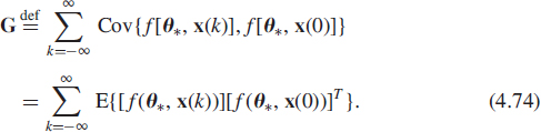
Note that all the eigenvalues of the derivative D of the mean field have strictly negative real parts since θ* is an asymptotically stable point of (4.69) and that for independent data x(k), G is simply the covariance of the field. Unless we have sufficient information about the data, which is often not the case, in practice we consider the simplifying hypothesis of independent identically Gaussian distributed data x(k).
It should be mentioned that the rigorous proof of this result (4.71) needs a very strong hypothesis on the algorithm (4.68), namely that θ(k) converges almost surely to the unique globally asymptotically stable point θ* in the corresponding decreasing step size algorithm. However, the practical use of (4.71) in more general situations is usually justified by using a general diffusion approximation result formally [13, Th. 1, p. 104].
In practice, μ is small and fixed, but it is assumed that the asymptotic distribution of ![]() when k tends to ∞ can still be approximated by a zero mean Gaussian distribution of covariance Cθ, and consequently that for large enough k, the distribution of the residual error (θμ(k) − θ*) is a zero mean Gaussian distribution of covariance μCθ where Cθ is solution of the Lyapunov equation (4.72). Note that the approximation
when k tends to ∞ can still be approximated by a zero mean Gaussian distribution of covariance Cθ, and consequently that for large enough k, the distribution of the residual error (θμ(k) − θ*) is a zero mean Gaussian distribution of covariance μCθ where Cθ is solution of the Lyapunov equation (4.72). Note that the approximation ![]() enables us to derive an expression of the asymptotic bias E[θμ(k)] − θ* from a perturbation analysis of the expectation of both sides of (4.68) when the field f[θ(k), x(k)] is linear in x(k)xT(k). An example of such a derivation is given in Subsection 4.7.3, [26] and Exercise 4.18.
enables us to derive an expression of the asymptotic bias E[θμ(k)] − θ* from a perturbation analysis of the expectation of both sides of (4.68) when the field f[θ(k), x(k)] is linear in x(k)xT(k). An example of such a derivation is given in Subsection 4.7.3, [26] and Exercise 4.18.
Finally, let us recall that there is no relation between the asymptotic performance of the stochastic approximation algorithm (4.68) and its convergence rate. As is well known, the convergence rate depends on the transient behavior of the algorithm, for which no general result seems to be available. For this reason, different authors (e.g. [22, 26]) have resorted to simulations to compare the convergence speed of different algorithms whose associated stepsizes μ are chosen to provide the same value of the mean square error ![]() .
.
4.7.3 Examples of Convergence and Performance Analysis
Using the previously described methods, two examples of convergence and performance analysis will be given. Oja's neuron algorithm as the simplest algorithm will allow us to present a comprehensive study of an eigenvector tracking algorithm. Then Oja's algorithm will be studied as an example of a subspace tracking algorithm.
Convergence and Performance Analysis of the Oja's Neuron Consider Oja's neuron algorithms (4.23) and (4.25) introduced in Section 4.4. The stationary points of their associated ODE
![]()
are the roots of Cxw = w[wTCxw] and thus are clearly given by (±uk)k=1,…, n. To study the stability of these stationarity points, consider the derivative Dw of the mean field Cxw − w[wTCxw] {resp., −Cxw + w[wTCxw]} at these points. Using a standard first-order perturbation, we obtain
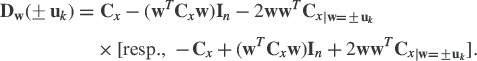
Because the eigenvalues of Dw(±uk) are −2λk, (λi − λk)i≠k [resp. 2λk, −(λi − λk)i≠k], these eigenvalues are all real negative for k = 1 only, for the stochastic approximation algorithms (4.23), in contrast to the stochastic approximation algorithms (4.25) for which Dw(±uk) has at least one nonnegative eigenvalue. Consequently only ±u1 is locally asymptotically stable for the ODE associated with (4.23) and all the eigenvectors (±uk)k=1,…, n are unstable for the ODE associated with (4.25) and thus only (4.23) (Oja's neuron for dominant eigenvector) can be retained.
Note that the coupled stochastic approximation algorithms (4.23) and (4.25) can be globally written as (4.68) as well. The associated ODE, given by
![]()
has the pairs (±uk, λk)k=1,…n as stationary points. The derivative D of the mean field at theses points is given by
![]()
whose eigenvalues are −2λk, (λi − λk)i≠k and − 1. Consequently the pair (±u1, λ1) is the only locally asymptotically stable point for the associated ODE (4.76) as well.
More precisely, it is proved in [50] that if w(0)Tu1 > 0 [resp. < 0], the solution w(t) of the ODE (4.69) tends exponentially to u1 [resp. −u1] as t → ∞. The pair (±u1, λ1) is thus globally asymptotically stable for the associated ODE.
Furthermore, using the stochastic approximation theory and in particular [44, Th. 2.3.1], it is proved in [51] that Oja's neuron (4.23) with decreasing stepsize μk, converges almost surely to +u1 or −u1 as k tends to ∞.
We have now the conditions to apply the Gaussian approximation results of Subsection 4.7.2. To solve the Lyapunov equation, the derivative D of the mean field at the pair (±u1, λ1) is given by
![]()
In the case of independent Gaussian distributed data x(k), it has been proved [22, 26] that the covariance G (4.74) of the field is given by
![]()
with ![]() . Solving the Lyapunov equation (4.72), the following asymptotic covariance Cθ is obtained [22, 26]
. Solving the Lyapunov equation (4.72), the following asymptotic covariance Cθ is obtained [22, 26]
![]()
with ![]() . Consequently the estimates [w(k), λ(k)] of (±u1, λ1) given by (4.23) and (4.24) respectively, are asymptotically independent and Gaussian distributed with
. Consequently the estimates [w(k), λ(k)] of (±u1, λ1) given by (4.23) and (4.24) respectively, are asymptotically independent and Gaussian distributed with

We note that the behavior of the adaptive estimates [w(k), λ(k)] of (±u1, λ1) are similar to the behavior of their batch estimates. More precisely if w(k) and λ(k) denote now the dominant eigenvector and the associated eigenvalue of the sample estimate ![]() of Cx, a standard result [3, Th. 13.5.1, p. 541] gives
of Cx, a standard result [3, Th. 13.5.1, p. 541] gives
![]()
with ![]() where
where ![]() . The estimates w(k) and λ(k) are asymptotically uncorrelated and the estimation of the eigenvalue λ1 is well conditioned in contrast to those of the eigenvector u1 whose conditioning may be very bad when λ1 and λ2 are very close.
. The estimates w(k) and λ(k) are asymptotically uncorrelated and the estimation of the eigenvalue λ1 is well conditioned in contrast to those of the eigenvector u1 whose conditioning may be very bad when λ1 and λ2 are very close.
Expressions of the asymptotic bias ![]() can be derived from (4.71). A word of caution is nonetheless necessary because the convergence of
can be derived from (4.71). A word of caution is nonetheless necessary because the convergence of ![]() to a limiting Gaussian distribution with covariance matrix Cθ does not guarantee the convergence of its moments to those of the limiting Gaussian distribution. In batch estimation, both the first and the second moments of the limiting distribution of
to a limiting Gaussian distribution with covariance matrix Cθ does not guarantee the convergence of its moments to those of the limiting Gaussian distribution. In batch estimation, both the first and the second moments of the limiting distribution of ![]() are equal to the corresponding asymptotic moments for independent Gaussian distributed data x(k). In the following, we assume the convergence of the second-order moments allowing us to write
are equal to the corresponding asymptotic moments for independent Gaussian distributed data x(k). In the following, we assume the convergence of the second-order moments allowing us to write
![]()
Let ![]() with
with ![]() . Provided the data x(k) are independent (which implies that w(k) and x(k)xT(k) are independent) and θμ(k) is stationary, taking the expectation of both sides of (4.23) and (4.24) gives11
. Provided the data x(k) are independent (which implies that w(k) and x(k)xT(k) are independent) and θμ(k) is stationary, taking the expectation of both sides of (4.23) and (4.24) gives11
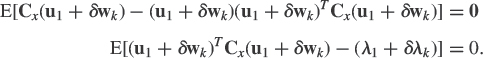
Using a second-order expansion, we get after some algebraic manipulations

Solving this equation in E(δwk) and E(δλk) using the expression of Cw, gives the following expressions of the asymptotic bias

We note that these asymptotic biases are similar to those obtained in batch estimation derived from a Taylor series expansion [77, p. 68] with expression (4.77) of Cθ.

Finally, we see that in adaptive and batch estimation, the square of these biases are an order of magnitude smaller that the variances in O(μ) or ![]() .
.
This methodology has been applied to compare the theoretical asymptotic performance of several adaptive algorithms for minor and principal component analysis in [22, 26, 27]. For example, the asymptotic mean square error ![]() of the estimate W(k) given by the WSA algorithm (4.57) is shown in Figure 4.1, where the stepsize μ is chosen to provide the same value for μTr(Cθ). We clearly see in this figure that the value β2/β1 = 0.6 optimizes the asymptotic mean square error/speed of convergence tradeoff.
of the estimate W(k) given by the WSA algorithm (4.57) is shown in Figure 4.1, where the stepsize μ is chosen to provide the same value for μTr(Cθ). We clearly see in this figure that the value β2/β1 = 0.6 optimizes the asymptotic mean square error/speed of convergence tradeoff.

Figure 4.1 Learning curves of the mean square error ![]() averaging 100 independent runs for the WSA algorithm, for different values of parameter β2/β1 = 0.96 (1), 0.9 (2), 0.1 (3), 0.2 (4), 0.4 (5), and 0.6 (6) compared with μTr(Cθ)(0) in the case n = 4, r = 2, Cx = Diag(1.75, 1.5, 0.5, 0.25), where the entries of W(0) are chosen randomly uniformly in [0, 1].
averaging 100 independent runs for the WSA algorithm, for different values of parameter β2/β1 = 0.96 (1), 0.9 (2), 0.1 (3), 0.2 (4), 0.4 (5), and 0.6 (6) compared with μTr(Cθ)(0) in the case n = 4, r = 2, Cx = Diag(1.75, 1.5, 0.5, 0.25), where the entries of W(0) are chosen randomly uniformly in [0, 1].
Convergence and Performance Analysis of Oja's Algorithm Consider now Oja's algorithm (4.30) described in Subsection 4.5.1. A difficulty arises in the study of the behavior of W(k) because the set of orthonormal bases of the r-dominant subspace forms a continuum of attractors: the column vectors of W(k) do not tend in general to the eigenvectors u1, …, ur, and we have no proof of convergence of W(k) to a particular orthonormal basis of their span. Thus, considering the asymptotic distribution of W(k) is meaningless. To solve this problem, in the same way as Williams [78] did when he studied the stability of the estimated projection matrix ![]() in the dynamics induced by Oja's learning equation
in the dynamics induced by Oja's learning equation ![]() , viz
, viz
![]()
we consider the trajectory of the matrix ![]() whose dynamics are governed by the stochastic equation
whose dynamics are governed by the stochastic equation
![]()
with ![]() and
and ![]() . A remarkable feature of (4.79) is that the field f and the complementary term h depend only on P(k) and not on W(k). This fortunate circumstance makes it possible to study the evolution of P(k) without determining the evolution of the underlying matrix W(k). The characteristics of P(k) are indeed the most interesting since they completely characterize the estimated subspace. Since (4.78) has a unique global asymptotically stable point P* = Πs [69], we can conjecture from the stochastic approximation theory [13, 44] that (4.79) converges almost surely to P*. And consequently the estimate W(k) given by (4.30) converges almost surely to the signal subspace in the meaning recalled in Subsection 4.2.4.
. A remarkable feature of (4.79) is that the field f and the complementary term h depend only on P(k) and not on W(k). This fortunate circumstance makes it possible to study the evolution of P(k) without determining the evolution of the underlying matrix W(k). The characteristics of P(k) are indeed the most interesting since they completely characterize the estimated subspace. Since (4.78) has a unique global asymptotically stable point P* = Πs [69], we can conjecture from the stochastic approximation theory [13, 44] that (4.79) converges almost surely to P*. And consequently the estimate W(k) given by (4.30) converges almost surely to the signal subspace in the meaning recalled in Subsection 4.2.4.
To evaluate the asymptotic distributions of the subspace projection matrix estimator given by (4.79), we must adapt the results of Subsection 4.7.2 because the parameter P(k) is here a n × n rank-r symmetric matrix. Furthermore, we note that some eigenvalues of the derivative of the mean field ![]() are positive real. To overcome this difficulty, let us now consider the following parametrization of P(k) in a neighborhood of P* introduced in [24, 25]. If {θij(P) | 1 ≤ i ≤ j ≤ n} are the coordinates of P − P* in the orthonormal basis
are positive real. To overcome this difficulty, let us now consider the following parametrization of P(k) in a neighborhood of P* introduced in [24, 25]. If {θij(P) | 1 ≤ i ≤ j ≤ n} are the coordinates of P − P* in the orthonormal basis ![]() defined by
defined by
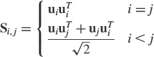
with the inner product under consideration is ![]() , then,
, then,
![]()
and θij(P) = Tr{Sij(P − P*)} for 1 ≤ i ≤ j ≤ n. The relevance of this basis is shown by the following relation proved in [24, 25]
![]()
where ![]() . There are
. There are ![]() pairs in Ps and this is exactly the dimension of the manifold of the n × n rank-r symmetric matrices. This point, together with relation (4.80), shows that the matrix set {Sij | (i,j) ∈ Ps} is in fact an orthonormal basis of the tangent plane to this manifold at point P*. In other words, a n × n rank-r symmetric matrix P lying less than ε away from P* (i.e., ||P − P*|| < ε) has negligible (of order ε2) components in the direction of Sij for r < i ≤ j ≤ n. It follows that, in a neighborhood of P*, the n × n rank-r symmetric matrices are uniquely determined by the
pairs in Ps and this is exactly the dimension of the manifold of the n × n rank-r symmetric matrices. This point, together with relation (4.80), shows that the matrix set {Sij | (i,j) ∈ Ps} is in fact an orthonormal basis of the tangent plane to this manifold at point P*. In other words, a n × n rank-r symmetric matrix P lying less than ε away from P* (i.e., ||P − P*|| < ε) has negligible (of order ε2) components in the direction of Sij for r < i ≤ j ≤ n. It follows that, in a neighborhood of P*, the n × n rank-r symmetric matrices are uniquely determined by the ![]() vector θ(P) defined by:
vector θ(P) defined by: ![]() , where
, where ![]() denotes the following
denotes the following ![]() matrix:
matrix: ![]() . If
. If ![]() denotes the unique (for ||θ|| sufficiently small) n × n rank-r symmetric matrix such that
denotes the unique (for ||θ|| sufficiently small) n × n rank-r symmetric matrix such that ![]() , the following one-to-one mapping is exhibited for sufficiently small ||θ(k)||
, the following one-to-one mapping is exhibited for sufficiently small ||θ(k)||

We are now in a position to solve the Lyapunov equation in the new parameter θ. The stochastic equation governing the evolution of θ(k) is obtained by applying the transformation ![]() to the original equation (4.79), thereby giving
to the original equation (4.79), thereby giving
![]()
where ![]() and
and ![]() .
.
Solving now the Lyapunov equation associated with (4.82) after deriving the derivative of the mean field ![]() and the covariance of the field ϕ[θ(k), x(k)] for independent Gaussian distributed data x(k), yields the covariance Cθ of the asymptotic distribution of θ(k). Finally using mapping (4.81), the covariance
and the covariance of the field ϕ[θ(k), x(k)] for independent Gaussian distributed data x(k), yields the covariance Cθ of the asymptotic distribution of θ(k). Finally using mapping (4.81), the covariance ![]() of the asymptotic distribution of P(k) is deduced [25]
of the asymptotic distribution of P(k) is deduced [25]

To improve the learning speed and misadjustment tradeoff of Oja's algorithm (4.30), it has been proposed in [25] to use the recursive estimate (4.20) for Cx(k) = E[x(k)xT(k)]. Thus the modified Oja's algorithm, called the smoothed Oja's algorithm, reads
![]()
![]()
where α is introduced in order to normalize both algorithms because if the learning rate of (4.84) has no dimension, the learning rate of (4.85) must have the dimension of the inverse of the power of x(k). Furthermore α can take into account a better tradeoff between the misadjustments and the learning speed. Note that the performance derivations may be extended to this smoothed Oja's algorithm by considering that the coupled stochastic approximation algorithms (4.84) and (4.85) can be globally written as (4.68) as well. Reusing now the parametrization (θij)1≤i≤j≤n because C(k) is symmetric as well, and following the same approach, we obtain now [25]

with ![]() .
.
This methodology has been applied to compare the theoretical asymptotic performance of several minor and principal subspace adaptive algorithms in [24, 25]. For example, the asymptotic mean square error ![]() of the estimate P(k) given by Oja's algorithm (4.30) and the smoothed Oja's algorithm (4.84) are shown in Figure 4.2, where the stepsize μ of the Oja's algorithm and the couple (μ, α) of the smoothed Oja's algorithm are chosen to provide the same value for μTr(CP). We clearly see in this figure that the smoothed Oja's algorithm with α = 0.3 provides faster convergence than the Oja's algorithm.
of the estimate P(k) given by Oja's algorithm (4.30) and the smoothed Oja's algorithm (4.84) are shown in Figure 4.2, where the stepsize μ of the Oja's algorithm and the couple (μ, α) of the smoothed Oja's algorithm are chosen to provide the same value for μTr(CP). We clearly see in this figure that the smoothed Oja's algorithm with α = 0.3 provides faster convergence than the Oja's algorithm.
Regarding the issue of asymptotic bias, note that there is a real methodological problem to apply the methodology of the end of Subsection 4.7.3. The trouble stems from the fact that the matrix P(k) = W(k)WT(k) does not belong to a linear vector space because it is constrained to have fixed rank r < n. The set of such matrices is not invariant under addition; it is actually a smooth submanifold of ![]() . This is not a problem in the first-order asymptotic analysis because this approach amounts to approximating this manifold by its tangent plane at a point of interest. This tangent plane is linear indeed. In order to refine the analysis by developing a higher order theory, it becomes necessary to take into account the curvature of the manifold. This is a tricky business. As an example of these difficulties, one could show (under simple assumptions) that there exists no projection-valued estimators of a projection matrix that are unbiased at order O(μ); this can be geometrically pictured by representing the estimates as points on a curved manifold (here: the manifold of projection matrices).
. This is not a problem in the first-order asymptotic analysis because this approach amounts to approximating this manifold by its tangent plane at a point of interest. This tangent plane is linear indeed. In order to refine the analysis by developing a higher order theory, it becomes necessary to take into account the curvature of the manifold. This is a tricky business. As an example of these difficulties, one could show (under simple assumptions) that there exists no projection-valued estimators of a projection matrix that are unbiased at order O(μ); this can be geometrically pictured by representing the estimates as points on a curved manifold (here: the manifold of projection matrices).
Using a more involved expression of the covariance of the field (4.74), the previously described analysis can be extended to correlated data x(k). Expressions (4.83) and (4.86) extend provided that λiλj is replaced by λiλj + λi,j where λi,j is defined in [25]. Note that when x(k) = (xk, xk−1, …, xk−n+1)T with xk being an ARMA stationary process, the covariance of the field (4.74) and thus λi,j can be expressed in closed form with the help of a finite sum [23].

Figure 4.2 Learning curves of the mean square error ![]() averaging 100 independent runs for the Oja's algorithm (1) and the smoothed Oja's algorithm with α = 1 (2) and α = 0.3 (3) compared with μTr(CP) (0) in the same configuration [Cx, W(0)] as Figure 4.1.
averaging 100 independent runs for the Oja's algorithm (1) and the smoothed Oja's algorithm with α = 1 (2) and α = 0.3 (3) compared with μTr(CP) (0) in the same configuration [Cx, W(0)] as Figure 4.1.
The domain of learning rate μ for which the previously described asymptotic approach is valid and the performance criteria for which no analytical results could be derived from our first-order analysis, such as the speed of convergence and the deviation from orthonormality ![]() can be derived from numerical experiments only. In order to compare Oja's algorithm and the smoothed Oja's algorithm, the associated parameters μ and (α, μ) must be constrained to give the same value of μTr(CP). In these conditions, it has been shown in [25] by numerical simulations that the smoothed Oja's algorithm provides faster convergence and a smaller deviation from orthonormality d2(μ) than Oja's algorithm. More precisely, it has been shown that d2(μ) ∝ μ2 [resp. ∝ μ4] for Oja's [resp. the smoothed Oja's] algorithm. This result agrees with the presentation of Oja's algorithm given in Subsection 4.5.1 in which the term
can be derived from numerical experiments only. In order to compare Oja's algorithm and the smoothed Oja's algorithm, the associated parameters μ and (α, μ) must be constrained to give the same value of μTr(CP). In these conditions, it has been shown in [25] by numerical simulations that the smoothed Oja's algorithm provides faster convergence and a smaller deviation from orthonormality d2(μ) than Oja's algorithm. More precisely, it has been shown that d2(μ) ∝ μ2 [resp. ∝ μ4] for Oja's [resp. the smoothed Oja's] algorithm. This result agrees with the presentation of Oja's algorithm given in Subsection 4.5.1 in which the term ![]() was omitted from the orthonormalization of the columns of W(k).
was omitted from the orthonormalization of the columns of W(k).
Finally, using the theorem of continuity (e.g. [59, Th. 6.2a]), note that the behavior of any differentiable function of P(k) can be obtained. For example, in DOA tracking from the MUSIC algorithm12 (see e.g. Subsection 4.8.1), the MUSIC estimates [θi(k)]i=1,…,r of the DOAs at time k can be determined as the r deepest minima of the localization function aH(θ)[In − P(k)]a(θ). Using the mapping ![]() where here
where here ![]() , the Gaussian asymptotic distribution of the estimate θ(k) can be derived [24] and compared to the batch estimate. For example for a single source, it has been proved [24] that
, the Gaussian asymptotic distribution of the estimate θ(k) can be derived [24] and compared to the batch estimate. For example for a single source, it has been proved [24] that
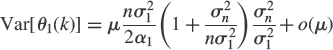
where ![]() is the source power and α1 is a purely geometrical factor. Compared to the batch MUSIC estimate
is the source power and α1 is a purely geometrical factor. Compared to the batch MUSIC estimate

the variances are similar provided ![]() is replaced by
is replaced by ![]() . This suggests that the stepsize μ of the adaptive algorithm must be normalized by
. This suggests that the stepsize μ of the adaptive algorithm must be normalized by ![]() .
.
4.8 ILLUSTRATIVE EXAMPLES
Fast estimation and tracking of the principal (or minor) subspace or components of a sequence of random vectors is a major tool for parameter and signal estimation in many signal processing communications and RADAR applications (see e.g. [11] and the references therein). We can cite, for example, the DOA tracking and the blind channel estimation including CDMA and OFDM communications as illustrations.
Going back to the common observation model (4.15) introduced in Subsection 4.3.1
![]()
where A(k) is an n × r full column rank matrix with r < n, the different applications are issued from specific deterministic parametrizations A[ϕ(k)] of A(k) where ![]() is a slowly time-varying parameter compared to r(k). When this parametrization
is a slowly time-varying parameter compared to r(k). When this parametrization ![]() is nonlinear, ϕ(k) is assumed identifiable from the signal subspace span[A(k)] or the noise subspace null[AT(k)] which is its orthogonal complement, that is,
is nonlinear, ϕ(k) is assumed identifiable from the signal subspace span[A(k)] or the noise subspace null[AT(k)] which is its orthogonal complement, that is,
![]()
and when this parametrization ![]() is linear, this identifiability is of course up to a multiplicative constant only.
is linear, this identifiability is of course up to a multiplicative constant only.
4.8.1 Direction of Arrival Tracking
In the standard narrow-band array data model, A(ϕ) is partitioned into r column vectors as ![]() , where (ϕi)i=1,…, r denotes different parameters associated with the r sources (azimuth, elevation, polarization, …). In this case, the parametrization is nonlinear. The simplest case corresponds to one parameter per source (q = r) (e.g. for a uniform linear array
, where (ϕi)i=1,…, r denotes different parameters associated with the r sources (azimuth, elevation, polarization, …). In this case, the parametrization is nonlinear. The simplest case corresponds to one parameter per source (q = r) (e.g. for a uniform linear array ![]() . For convenience and without loss of generality, we consider this case in the following. A simplistic idea to track the r DOAs would be to use an adaptive estimate
. For convenience and without loss of generality, we consider this case in the following. A simplistic idea to track the r DOAs would be to use an adaptive estimate ![]() of the noise orthogonal projection matrix Πn(k) given by W(k)WT(k) or In − W(k)WT(k) where W(k) is, respectively, given by a minor or a dominant subspace adaptive algorithm introduced in Section 4.5,13 and then to derive the estimated DOAs as the r minima of the cost function
of the noise orthogonal projection matrix Πn(k) given by W(k)WT(k) or In − W(k)WT(k) where W(k) is, respectively, given by a minor or a dominant subspace adaptive algorithm introduced in Section 4.5,13 and then to derive the estimated DOAs as the r minima of the cost function
![]()
by a Newton–Raphson procedure

where ![]() and
and ![]() . While this approach works for distant different DOAs, it breaks down when the DOAs of two or more sources are very close and particularly in scenarios involving targets with crossing trajectories. So the difficulty in DOA tracking is the association of the DOA estimated at different time points with the correct sources. To solve this difficulty, various algorithms for DOA tracking have been proposed in the literature (see e.g. [60] and the references therein). To maintain this correct association, a solution is to introduce the dynamic model governing the motion of the different sources
. While this approach works for distant different DOAs, it breaks down when the DOAs of two or more sources are very close and particularly in scenarios involving targets with crossing trajectories. So the difficulty in DOA tracking is the association of the DOA estimated at different time points with the correct sources. To solve this difficulty, various algorithms for DOA tracking have been proposed in the literature (see e.g. [60] and the references therein). To maintain this correct association, a solution is to introduce the dynamic model governing the motion of the different sources
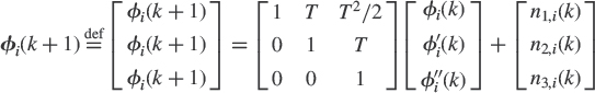
where T denotes the sampling interval and [nj,i(k)]j=1,2,3 are random process noise terms that account for random perturbations about the constant acceleration trajectory. This enables us to predict the state (position, velocity, and acceleration) of each source in any interval of time using the estimated state in the previous interval. An efficient and computationally simple heuristic procedure has been proposed in [66]. It consists of four steps by iteration k. First, a prediction ![]() of the state from the estimate
of the state from the estimate ![]() is obtained. Second, an update of the estimated noise projection matrix
is obtained. Second, an update of the estimated noise projection matrix ![]() given by a subspace tracking algorithm introduced in Section 4.5 is derived from the new snapshot x(k). Third, for each source i, an estimate
given by a subspace tracking algorithm introduced in Section 4.5 is derived from the new snapshot x(k). Third, for each source i, an estimate ![]() given by a Newton–Raphson step initialized by the predicted DOA
given by a Newton–Raphson step initialized by the predicted DOA ![]() given by a Kalman filter of the first step whose measurement equation is given by
given by a Kalman filter of the first step whose measurement equation is given by
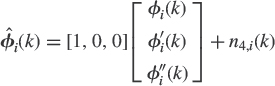
where the observation ![]() is the DOA estimated by the Newton–Raphson step at iteration k − 1. Finally, the DOA
is the DOA estimated by the Newton–Raphson step at iteration k − 1. Finally, the DOA ![]() predicted by the Kalman filter is also used to smooth the DOA
predicted by the Kalman filter is also used to smooth the DOA ![]() estimated by the Newton–Raphson step, to give the new estimate
estimated by the Newton–Raphson step, to give the new estimate ![]() of the state whose its first component is used for tracking the r DOAs.
of the state whose its first component is used for tracking the r DOAs.
4.8.2 Blind Channel Estimation and Equalization
In communication applications, the matched filtering followed by symbol rate sampling or oversampling yields an n-vector data x(k) which satisfies the model (4.87), where r(k) contains different transmitted symbols bk. Depending on the context, (SIMO channel or CDMA, OFDM, MC CDMA) with or without intersymbol interference, different parametrizations of A(k) arise which are generally linear in the unknown parameter ϕ(k). The latter represents different coefficients of the impulse response of the channel that are assumed slowly time-varying compared to the symbol rate. In these applications, two problems arise. First, the updating of the estimated parameters ϕ(k), that is, the adaptive identification of the channel can be useful to an optimal equalization based on an identified channel. Second, for particular models (4.87), a direct linear equalization mT(k)x(k) can be used from the adaptive estimation of the weight m(k). To illustrate subspace or component-based methods, two simple examples are given in the following.
For the two channel SIMO model, we assume that the two channels are of order m and that we stack the m + 1 most recent samples of each channel to form the observed data x(k) = [x1(k), x2(k)]T. In this case we obtain the model (4.87) where A(k) is the following 2(m + 1) × (2 m + 1) Sylvester filtering matrix

and r(k) = (bk, …, bk−2m)T, with ϕi(k) = [hi,1(k), hi,2(k)]T, i = 0, … m where hi,j represents the ith term of the impulse response of the j-th channel. These two channels do not share common zeros, guaranteeing their identifiability. In this specific two-channel case, the so called least square [80] and subspace [49] estimates of the impulse response ![]() defined up to a constant scale factor, coincide [81] and are given by ϕ(k) = Tv(k) with v(k) is the eigenvector associated with the unique smallest eigenvalue of Cx(k) = E[x(k)xT(k)] where T is the antisymmetric orthogonal matrix
defined up to a constant scale factor, coincide [81] and are given by ϕ(k) = Tv(k) with v(k) is the eigenvector associated with the unique smallest eigenvalue of Cx(k) = E[x(k)xT(k)] where T is the antisymmetric orthogonal matrix ![]() . Consequently an adaptive estimation of the slowly time-varying impulse response ϕ(k) can be derived from the adaptive estimation of the eigenvector v(k). Note that in this example, the rank r of the signal subspace is given by r = 2 m + 1 whose order m of the channels that usually possess small leading and trailing terms is ill defined. For such channels it has been shown [46] that blind channel approximation algorithms should attempt to model only the significant part of the channel composed of the large impulse response terms because efforts toward modeling small leading and/or trailing terms lead to effective over-modeling, which is generically ill-conditioned and, thus, should be avoided. A detection procedure to detect the order of this significant part has been given in [45].
. Consequently an adaptive estimation of the slowly time-varying impulse response ϕ(k) can be derived from the adaptive estimation of the eigenvector v(k). Note that in this example, the rank r of the signal subspace is given by r = 2 m + 1 whose order m of the channels that usually possess small leading and trailing terms is ill defined. For such channels it has been shown [46] that blind channel approximation algorithms should attempt to model only the significant part of the channel composed of the large impulse response terms because efforts toward modeling small leading and/or trailing terms lead to effective over-modeling, which is generically ill-conditioned and, thus, should be avoided. A detection procedure to detect the order of this significant part has been given in [45].
Consider now an asynchronous direct sequence CDMA system of r users without intersymbol interference. In this case, model (4.87) applies, where A(k) is given by
![]()
where ai(k) and si are respectively the amplitude and the signature sequence of the i-th user and r(k) = (bk,1, …, bk,r)T where bk,i is the symbol k of the i-th user. We assume that only the signature sequence of User 1, the user of interest, is known. Two linear multiuser detectors mT(k)x(k), namely, the decorrelation detector (i.e., that completely eliminates the multiple access interference caused by the other users) and the linear MMSE detector for estimating the symbol bk,1, have been proposed in [76] in terms of the signal eigenvalues and eigenvectors. The scaled version of the respective weights m(k) of these detectors are given by
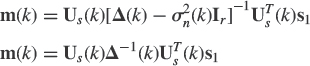
where Us(k) = [v1(k), …, vr(k)], Δ(k) = Diag[λ1(k), …, λr(k)] and ![]() issued from the adaptive EVD of Cx(k) = E[x(k)xT(k)] including the detection of the number r of user that can change by a rank tracking procedure (e.g. [72]).
issued from the adaptive EVD of Cx(k) = E[x(k)xT(k)] including the detection of the number r of user that can change by a rank tracking procedure (e.g. [72]).
4.9 CONCLUDING REMARKS
Although adaptive subspace and component-based algorithms were introduced in signal processing three decades ago, a rigorous convergence analysis has been derived only for the celebrated Oja's algorithm, whose Oja's neuron is a particular case, in stationary environments. In general all of these techniques are derived heuristically from standard iterative computational techniques issued from numerical methods of linear algebra. So a theoretical convergence and performance analysis of these algorithms is necessary, but seems very challenging. Furthermore, such analysis is not sufficient because these algorithms may present numerical instabilities due to rounding errors. Consequently, a comprehensive comparison of the different algorithms that have appeared in the literature from the performance (convergence speed, mean square error, distance to the orthonormality, tracking capabilities), computational complexity and numerical stability points of view—that are out the scope of this chapter—would be be very useful for practitioners.
The interest of the signal processing community in adaptive subspace and component-based schemes remains strong as is evident from the numerous articles and reports published in this area each year. But we note that these contributions mainly consist in the application of standard adaptive subspace and component-based algorithms in new applications and in refinements of well known subspace/component-based algorithms, principally to reduce their computational complexity and to numerically stabilize the minor subspace/component-based algorithms, whose literature is much more limited than the principal subspace and component-based algorithms.
4.10 PROBLEMS
4.1 Let λ0 be a simple eigenvalue of a real symmetric n × n matrix C0, and let u0 be a unit 2-norm associated eigenvector, so that Cu0 = λ0u0. Then a real-valued function λ(.) and a vector function u(.) are defined for all C in some neighborhood (e.g. among the real symmetric matrices) of C0 such that
![]()
Using simple perturbations algebra manipulations, prove that the functions λ(.) and u(.) are differentiable on some neighborhood of C0 and that the differentials at C0 are given by
![]()
where # stands for the Moore Penrose inverse. Prove that if the constraint ||u||2 = 1 is replaced by ![]() , the differential δu given by (4.88) remains valid.
, the differential δu given by (4.88) remains valid.
Now consider the same problem where C0 is a Hermitian matrix. To fix the perturbed eigenvector u, the condition ||u||2 = 1 is not sufficient. So suppose now that ![]() . Note that in this case u no longer has unit 2-norm. Using the same approach as for the real symmetric case, prove that the functions λ(.) and u(.) are differentiable on some neighborhood of C0 and that the differentials at C0 are now given by
. Note that in this case u no longer has unit 2-norm. Using the same approach as for the real symmetric case, prove that the functions λ(.) and u(.) are differentiable on some neighborhood of C0 and that the differentials at C0 are now given by
![]()
In practice, different constraints are used to fix u. For example, the SVD function of MATLAB forces all eigenvectors to be unit 2-norm with a real first element. Specify in this case the new expression of the differential δu given by (4.89). Finally, show that the differential δu given by (4.88) would be obtained with the condition ![]() , which is no longer derived from the constraint ||u||2 = 1.
, which is no longer derived from the constraint ||u||2 = 1.
4.2 Consider an n × n real symmetric or complex Hermitian matrix C0 whose the r smallest eigenvalues are equal to σ2 with λn−r > λn−r+1. Let Π0 the projection matrix onto the invariant subspace associated with σ2. Then a matrix-valued function Π(.) is defined as the projection matrix onto the invariant subspace associated with the r smallest eigenvalues of C for all C in some neighborhood of C0 such that Π(C0) = Π0. Using simple perturbations algebra manipulations, prove that the functions Π(.) is two times differentiable on some neighborhood of C0 and that the differentials at C0 are given by
where ![]() .
.
4.3 Consider a Hermitian matrix C whose real and imaginary parts are denoted by Cr and Ci respectively. Prove that each eigenvalue eigenvector pair (λ, u) of C is associated with the eigenvalue eigenvector pairs ![]() and
and ![]() of the real symmetric matrix
of the real symmetric matrix ![]() where ur and ui denote the real and imaginary parts of u.
where ur and ui denote the real and imaginary parts of u.
4.4 Consider what happens when the orthogonal iteration method (4.11) is applied with r = n and under the assumption that all the eigenvalues of C are simple. The QR algorithm arises by considering how to compute the matrix ![]() directly from this predecessor Ti−1. Prove that the following iterations
directly from this predecessor Ti−1. Prove that the following iterations
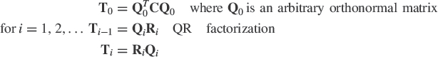
produce a sequence (Ti, Q0Qi…Qi) that converges to (Diag(λ1, …, λn), [±u1, …, ±un]).
4.5 Specify what happens to the convergence and the convergence speed, if the step Wi = orthonorm{CWi−1} of the orthogonal iteration algorithm (4.11) is replaced by the following {Wi = orthonorm{(In + μC)Wi−1}. Same questions, for the step {Wi = orthonormalization of C−1 Wi−1}, then {Wi = orthonormalization of (In − μC)Wi−1}. Specify the conditions that must satisfy the eigenvalues of C and μ for these latter two steps. Examine the specific case r = 1.
4.6 Using the EVD of C, prove that the solutions W of the maximizations and minimizations (4.7) are given by W = [u1, …, ur] Q and W = [un−r+1, …, un] Q respectively, where Q is an arbitrary r × r orthogonal matrix.
4.7 Consider the scalar function (4.14) ![]() of W = [w1, …, wr] with
of W = [w1, …, wr] with ![]() . Let ∇W = [∇1, …, ∇r] where (∇k)k=1,…, r is the gradient operator with respect to wk. Prove that
. Let ∇W = [∇1, …, ∇r] where (∇k)k=1,…, r is the gradient operator with respect to wk. Prove that
![]()
Then, prove that the stationary points of J(W) are given by W = UrQ where the r columns of Ur denote arbitrary r distinct unit-2 norm eigenvectors among u1, …, un of C and where Q is an arbitrary r × r orthogonal matrix. Finally, prove that at each stationary point, J(W) equals the sum of eigenvalues whose eigenvectors are not involved in Ur.
Consider now the complex valued case where ![]() with
with ![]() and use the complex gradient operator (see e.g., [36]) defined by
and use the complex gradient operator (see e.g., [36]) defined by ![]() where ∇R and ∇I denote the gradient operators with respect to the real and imaginary parts. Show that ∇WJ has the same form as the real gradient (4.90) except for a factor 1/2 and changing the transpose operator by the conjugate transpose one. By noticing that ∇wJ = O is equivalent to ∇R J = ∇I J = O, extend the previous results to the complex valued case.
where ∇R and ∇I denote the gradient operators with respect to the real and imaginary parts. Show that ∇WJ has the same form as the real gradient (4.90) except for a factor 1/2 and changing the transpose operator by the conjugate transpose one. By noticing that ∇wJ = O is equivalent to ∇R J = ∇I J = O, extend the previous results to the complex valued case.
4.8 With the notations of Exercise 4.7, suppose now that λr > λr+1 and consider first the real valued case. Show that the (i, j)th block ![]() of the block Hessian matrix H of J(W) with respect to the nr-dimensional vector
of the block Hessian matrix H of J(W) with respect to the nr-dimensional vector ![]() is given by
is given by

After evaluating the EVD of the block Hessian matrix H at the stationary points W= UrQ, prove that H is nonnegative if Ur = [u1, …, ur]. Interpret in this case the zero eigenvalues of H. Prove that when Ur contains an eigenvector different from u1, …, ur, some eigenvalues of H are strictly negative. Deduce that all stationary points of J(W) are saddle points except the points W whose associated matrix Ur contains the r dominant eigenvectors u1, …, ur of C which are global minima of the cost function (4.14).
Extend the previous results by considering the 2nr × 2nr real Hessian matrix ![]() with
with ![]() .
.
4.9 With the notations of the NP3 algorithm described in Subsection 4.5.1, write (4.40) in the form
![]()
with ![]() ,
, ![]() and
and ![]() . Then, using the EVD
. Then, using the EVD ![]() of the symmetric rank two matrix abT + baT + αaaT, prove equalities (4.41) and (4.42) where
of the symmetric rank two matrix abT + baT + αaaT, prove equalities (4.41) and (4.42) where ![]() .
.
4.10 Consider the following stochastic approximation algorithm derived from Oja's algorithm (4.30) where the sign of the step size can be reversed and where the estimate W(k) is forced to be orthonormal at each time step

where ![]() denotes the symmetric inverse square root of
denotes the symmetric inverse square root of ![]() . To compute the later, use the updating equation of W′(k + 1) and keeping in mind that W(k) is orthonormal, prove that
. To compute the later, use the updating equation of W′(k + 1) and keeping in mind that W(k) is orthonormal, prove that ![]() with
with ![]() where
where ![]() Using identity (4.5.9), prove that
Using identity (4.5.9), prove that ![]()
![]() with
with ![]()
![]() . Finally, using the update equation of W(k + 1), prove that algorithm (4.9.5) leads to W(k + 1) = W(k) ±μk p(k)yT(k) with
. Finally, using the update equation of W(k + 1), prove that algorithm (4.9.5) leads to W(k + 1) = W(k) ±μk p(k)yT(k) with ![]() .
.
Alternatively, prove that algorithm (4.9.5) leads to W(k + 1) = H(k)W(k) where H(k) is the Householder transform given by H(k) = In − 2u(k)uT(k) where ![]() .
.
4.11 Consider the scalar function (4.5.21) ![]() . Using the notations of Exercise 4.7, prove that
. Using the notations of Exercise 4.7, prove that
![]()
Then, prove that the stationary points of J(W) are given by W = Ur Q where the r columns of Ur denotes arbitrary r distinct unit-2 norm eigenvectors among u1, …, un of C and where Q is an arbitrary r × r orthogonal matrix. Finally, prove that at each stationary point, ![]() , where the r eigenvalues λsi are associated with the eigenvectors involved in Ur.
, where the r eigenvalues λsi are associated with the eigenvectors involved in Ur.
4.12 With the notations of Exercise 4.11 and using the matrix differential method [47, Chap. 6], prove that the Hessian matrix H of J(W) with respect to the nr-dimensional vector ![]() is given by
is given by
where Krn is the nr × rn commutation matrix [47, Chap. 2]. After evaluating this Hessian matrix H at the stationnary points W = UrQ of J(W) (4.46), substituting the EVD of C and deriving the EVD of H, prove that when λr > λr+1, H is nonnegative if Ur = [u1, …, ur]. Interpret in this case the zero eigenvalues of H. Prove that when Ur contains an eigenvector different from u1, …, ur, some eigenvalues of H are strictly positive. Deduce that all stationary points of J(W) are saddle points except the points W whose associated matrix Ur contains the r dominant eigenvectors u1, …, ur of C which are global maxima of the cost function (4.46).
4.13 Suppose the columns [w1(k), …, wr(k)] of the n × r matrix W(k) are orthonormal and let W′(k + 1) be the matrix W(k) ±μkx(k)xT(k)W(k). If the matrix S(k + 1) performs a Gram-Schmidt orthonormalization on the columns of W′(k + 1), write this in explicit form for the columns of matrix W(k + 1) = W′(k + 1)S(k + 1) as a power series expansion in μk and prove that
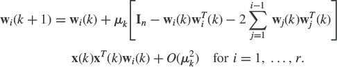
Following the same approach with now W′(k + 1) = W(k) ±x(k)xT(k)W(k)Γ(k) where Γ(k) = μkDiag(1, α2, …, αr), prove that
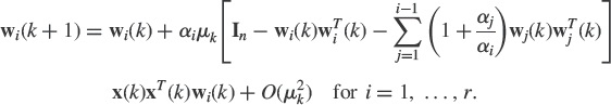
4.14 Specify the stationary points of the ODE associated with algorithm (4.58). Using the eigenvalues of the derivative of the mean field of this algorithm, prove that if λn−r+1 < 1 and ![]() , the only asymptotically stable points of the associated ODE are the eigenvectors ±vn−r+1, …, ±vn.
, the only asymptotically stable points of the associated ODE are the eigenvectors ±vn−r+1, …, ±vn.
4.15 Prove that the set of the n × r orthogonal matrices W (denoted the Stiefel manifold Stn,r) is given by the set of matrices of the form eAW where W is an arbitrary n × r fixed orthogonal matrix and A is a skew-symmetric matrix (AT = −A).
Prove the following relation
![]()
where J(W) = Tr[WH1WTH2] (where H1 and H2 are arbitrary r × r and n × n symmetric matrices) defined on the set of n × r orthogonal matrices. Then, give the differential dJ of the cost function J(W) and deduce the gradient of J(W) on this set of n × r orthogonal matrices
![]()
4.16 Prove that if ![]() , where J(θ) is a positive scalar function, J[θ(t)] tends to a constant as t tends to ∞, and consequently all the trajectories of the ODE (4.69) converge to the set of the stationary points of the ODE.
, where J(θ) is a positive scalar function, J[θ(t)] tends to a constant as t tends to ∞, and consequently all the trajectories of the ODE (4.69) converge to the set of the stationary points of the ODE.
4.17 Let θ* be a stationary point of the ODE (4.69). Consider a Taylor series expansion of ![]() about the point θ = θ*
about the point θ = θ*
![]()
By admitting that the behavior of the trajectory θ(t) of the ODE (4.69) in the neighborhood of θ* is identical to those of the associated linearized ODE  about the point θ*, relate the stability of the stationary point θ* to the behavior of the eigenvalues of the matrix D.
4.18 Consider the general stochastic approximation algorithm (4.68) in which the field f[θ(k), x(k)xT(k)] and the residual perturbation term h[θ(k), x(k)xT(k)] depend on the data x(k) through x(k) xT(k) and are linear in x(k)xT(k). The data x(k) are independent. The estimated parameter is here denoted ![]() . We suppose that the Gaussian approximation result (4.7.4) applies and that the convergence of the second-order moments allows us to write
. We suppose that the Gaussian approximation result (4.7.4) applies and that the convergence of the second-order moments allows us to write ![]() . Taking the expectation of both sides of (4.7.1), provided μk = μ and θμ(k) stationary, gives that
. Taking the expectation of both sides of (4.7.1), provided μk = μ and θμ(k) stationary, gives that
![]()
Deduce a general expression of the asymptotic bias ![]() .
.
REFERENCES
1. K. Abed Meraim, A. Chkeif, and Y. Hua, Fast orthogonal PAST algorithm, IEEE Signal Process. letters, 7, No. 3, pp. 60–62, (2000).
2. K. Abed Meraim, S. Attallah, A. Chkeif, and Y. Hua, Orthogonal Oja algorithm, IEEE Signal Process. letters, 7, No. 5, pp. 116–119, (2000).
3. T. W. Anderson, An introduction to multivariate statistical analysis, Second Edition, Wiley and Sons, 1984.
4. S. Attallah and K. Abed Meraim, Fast algorithms for subspace tracking, IEEE Signal Process. letters, 8, No. 7, pp. 203–206, (2001).
5. S. Attallah and K. Abed Meraim, Low cost adaptive algorithm for noise subspace estimation, Electron. letters, 48, No. 12, pp. 609–611, (2002).
6. S. Attallah, The generalized Rayleigh's quotient adaptive noise subspace algorithm: a Householder transformation-based implementation, IEEE Trans. on circ. and syst. II, 53, No. 81, pp. 3–7, (2006).
7. S. Attallah, J. H. Manton, and K. Abed Meraim, Convergence analysis of the NOJA algorithm using the ODE approach, Signal Processing, 86, pp. 3490–3495, (2006).
8. R. Badeau, B. David, and G. Richard, Fast approximated power iteration subspace tracking, IEEE Trans. on Signal Process., 53, No. 8, pp. 2931–2941, (2005).
9. S. Bartelmaos, K. Abed Meraim and S. Attallah, “Fast algorithms for minor component analysis,” Proc. ICASSP, Philadelphia, March 2005.
10. S. Bartelmaos, “Subspace tracking and mobile localization in UMTS,” Unpublished doctoral thesis, Telecom Paris and University Pierre et Marie Curie, France, 2008.
11. S. Beau and S. Marcos, Range dependent clutter rejection using range recursive space time adaptive processing (STAP) algorithms, Submitted to Signal Processing, March 2008.
12. R. Bellman, Stability theory of differential equations, McGraw Hill, New York, 1953.
13. A. Benveniste, M. Métivier, and P. Priouret, Adaptive algorithms and stochastic approximations, Springer Verlag, New York, 1990.
14. A. Cantoni and P. Butler, Eigenvalues and eigenvectors of symmetric centrosymmetric matrices, Linear Algebra and its Applications 13, pp. 275–288, (1976).
15. T. Chen, Modified Oja's algorithms for principal subspace and minor subspace extraction, Neural Processing letters, 5, pp. 105–110, (1997).
16. T. Chen, Y. Hua, and W. Y. Yan, Global convergence of Oja's subspace algorithm for principal component extraction, IEEE Trans. on Neural Networks, 9, No. 1, pp. 58–67, (1998).
17. T. Chen and S. Amari, Unified stabilization approach to principal and minor components extraction algorithms, Neural Networks, 14, No. 10, pp. 1377–1387, (2001).
18. T. Chonavel, B. Champagne, and C. Riou, Fast adaptive eigenvalue decomposition: a maximum likelihood approach, Signal Processing, 83, pp. 307–324, (2003).
19. A. Cichocki and S. Amari, Adaptive blind signal and image processing, learning algorithms and applications, John Wiley and Sons, 2002.
20. P. Comon and G. H. Golub, Tracking a few extreme singular values and vectors in signal processing, Proc. IEEE, 78, No. 8, pp. 1327–1343, (1990).
21. J. Dehaene, “Continuous-time matrix algorithms, systolic algorithms and adaptive neural networks,” Unpublished doctoral dissertation, Katholieke Univ. Leuven, Belgium, 1995.
22. J. P. Delmas and F. Alberge, Asymptotic performance analysis of subspace adaptive algorithms introduced in the neural network literature, IEEE Trans. on Signal Process., 46, No. 1, pp. 170–182, (1998).
23. J. P. Delmas, Performance analysis of a Givens parameterized adaptive eigenspace algorithm, Signal Processing, 68, No. 1, pp. 87–105, (1998).
24. J. P. Delmas and J. F. Cardoso, Performance analysis of an adaptive algorithm for tracking dominant subspace, IEEE Trans. on Signal Process., 46, No. 11, pp. 3045–3057, (1998).
25. J. P. Delmas and J. F. Cardoso, Asymptotic distributions associated to Oja's learning equation for Neural Networks, IEEE Trans. on Neural Networks, 9, No. 6, pp. 1246–1257, (1998).
26. J. P. Delmas, On eigenvalue decomposition estimators of centro-symmetric covariance matrices, Signal Processing, 78, No. 1, pp. 101–116, (1999).
27. J. P. Delmas and V. Gabillon, “Asymptotic performance analysis of PCA algorithms based on the weighted subspace criterion,” in Proc. ICASSP Taipei, Taiwan, April 2009.
28. S. C. Douglas, S. Y. Kung, and S. Amari, A self-stabilized minor subspace rule, IEEE Signal Process. letters, 5, No. 12, pp. 328–330, (1998).
29. X. G. Doukopoulos, “Power techniques for blind channel estimation in wireless communications systems,” Unpublished doctoral dissertation, IRISA-INRIA, University of Rennes, France, 2004.
30. X. G. Doukopoulos and G. V. Moustakides, “The fast data projection method for stable subspace tracking,” Proc. 13th European Signal Proc. Conf., Antalya, Turkey, September 2005.
31. X. G. Doukopoulos and G. V. Moustakides, Fast and Stable Subspace Tracking, IEEE Trans. on Signal Process, 56, No. 4, pp. 1452–1465, (2008).
32. J. C. Fort and G. Pagès, “Sur la convergence presque sure d'algorithmes stochastiques: le théoreme de Kushner-Clark theorem revisité,” Technical report, University Paris 1, 1994. Preprint SAMOS.
33. J. C. Fort and G. Pagès, Convergence of stochastic algorithms: from the Kushner and Clark theorem to the Lyapunov functional method, Advances in Applied Probability, No. 28, pp. 1072–1094, (1996).
34. B. Friedlander and A. J. Weiss, On the second-order of the eigenvectors of sample covariance matrices, IEEE Trans. on Signal Process., 46, No. 11, pp. 3136–3139, (1998).
35. G. H. Golub and C. F. Van Loan, Matrix computations, 3rd ed., the Johns Hopkins University Press, 1996.
36. S. Haykin, Adaptive filter theory, Englewoods Cliffs, NJ: Prentice Hall, 1991.
37. R. A. Horn and C. R. Johnson, Matrix analysis, Cambridge University Press, 1985.
38. Y. Hua, Y. Xiang, T. Chen, K. Abed Meraim, and Y. Miao, A new look at the power method for fast subspace tracking, Digital Signal Process., 9, No. 2, pp. 297–314, (1999).
39. B. H. Juang, S. Y. Kung, and C. A. Kamm (Eds.), Proc. IEEE Workshop on neural networks for signal processing, Princeton, NJ, September 1991.
40. I. Karasalo, Estimating the covariance matrix by signal subspace averaging, IEEE Trans. on on ASSP, 34, No. 1, pp. 8–12, (1986).
41. J. Karhunen and J. Joutsensalo, Generalizations of principal componant analysis, optimizations problems, and neural networks, Neural Networks, 8, pp. 549–562, (1995).
42. S. Y. Kung and K. I. Diamantaras, Adaptive principal component extraction (APEX) and applications, IEEE Trans. on ASSP, 42, No. 5, pp. 1202–1217, (1994).
43. H. J. Kushner and D. S. Clark, Stochastic approximation for constrained and unconstrained systems, Applied math. Science, No. 26, Springer Verlag, New York, 1978.
44. H. J. Kushner, Weak convergence methods and singular perturbed stochastic control and filtering problems, Vol. 3 of Systems and Control: Foundations and applications, Birkhäuser, 1989.
45. A. P. Liavas, P. A. Regalia, and J. P. Delmas, Blind channel approximation: Effective channel order determination, IEEE Transactions on Signal Process., 47, No. 12, pp. 3336–3344, (1999).
46. A. P. Liavas, P. A. Regalia, and J. P. Delmas, On the robustness of the linear prediction method for blind channel identification with respect to effective channel undermodeling/overmodeling, IEEE Transactions on Signal Process., 48, No. 5, pp. 1477–1481, (2000).
47. J. R. Magnus and H. Neudecker, Matrix differential calculus with applications in statistics and econometrics, Wiley series in probability and statistics, 1999.
48. Y. Miao and Y. Hua, Fast subspace tracking and neural learning by a novel information criterion, IEEE Trans. on Signal Process., 46, No. 7, pp. 1967–1979, (1998).
49. E. Moulines, P. Duhamel, J. F. Cardoso, and S. Mayrargue, Subspace methods for the blind identification of multichannel FIR filters, IEEE Trans. Signal Process., 43, No. 2, pp. 516–525, (1995).
50. E. Oja, A simplified neuron model as a principal components analyzer, J. Math. Biol., 15, pp. 267–273, (1982).
51. E. Oja and J. Karhunen, On stochastic approximation of the eigenvectors and eigenvalues of the expectation of a random matrix, J. Math. anal. Applications, 106, pp. 69–84, (1985).
52. E. Oja, Subspace methods of pattern recognition, Letchworth, England, Research Studies Press and John Wiley and Sons, 1983.
53. E. Oja, Principal components, minor components and linear neural networks, Neural networks, 5, pp. 927–935, (1992).
54. E. Oja, H. Ogawa, and J. Wangviwattana, Principal component analysis by homogeneous neural networks, Part I: The weighted subspace criterion, IEICE Trans. Inform. and Syst., E75-D, pp. 366–375, (1992).
55. E. Oja, H. Ogawa, and J. Wangviwattana, Principal component analysis by homogeneous neural networks, Part II: Analysis and extensions of the learning algorithms, IEICE Trans. Inform. Syst., E75-D, pp. 376–382, (1992).
56. N. Owsley, “Adaptive data orthogonalization,” in Proc. Conf. ICASSP, pp. 109–112, 1978.
57. B. N. Parlett, The symmetric eigenvalue problem, Prentice Hall, Englewood Cliffs, N.J. 1980.
58. B. Picinbono, Second-order complex random vectors and normal distributions, IEEE Trans. on Signal Process., 44, No. 10, pp. 2637–2640, (1996).
59. C. R. Rao, Linear statistical inference and its applications, New York, Wiley, 1973.
60. C. R. Rao, C. R. Sastry, and B. Zhou, Tracking the direction of arrival of moving targets, IEEE Trans. on Signal Process., 472, No. 5, pp. 1133–1144, (1994).
61. P. A. Regalia, An adaptive unit norm filter with applications to signal analysis and Karhunen Loéve tranformations, IEEE Trans. on Circuits and Systems, 37, No. 5, pp. 646–649, (1990).
62. C. Riou, T. Chonavel, and P. Y. Cochet, “Adaptive subspace estimation – Application to moving sources localization and blind channel identification,” in Proc. ICASSP Atlanta, GA, May 1996.
63. C. Riou, “Estimation adaptative de sous espaces et applications,” Unpublished doctoral dissertation, ENSTB, University of Rennes, France, 1997.
64. H. Rutishauser, Computational aspects of F. L. Bauer's simultaneous iteration method, Numer. Math, 13, pp. 3–13, (1969).
65. H. Sakai and K. Shimizu, A new adaptive algorithm for minor component analysis, Signal Processing, 71, pp. 301–308, (1998).
66. J. Sanchez-Araujo and S. Marcos, A efficient PASTd algorithm implementation for multiple direction of arrival tracking, IEEE Trans. on Signal Process., 47, No. 8, pp. 2321–2324, (1999).
67. T. D. Sanger, Optimal unsupervised learning in a single-layer linear feedforward network, Neural Networks, 2, pp. 459–473, (1989).
68. A. H. Sayed, Fundamentals of adaptive filtering, IEEE Press, Wiley-Interscience, 2003.
69. W. Y. Yan, U. Helmke, and J. B. Moore, Global analysis of Oja's flow for neural networks, IEEE Trans. on Neural Networks, 5, No. 5, pp. 674–683, (1994).
70. J. F. Yang and M. Kaveh, Adaptive eigensubspace algorithms for direction or frequency estimation and tracking, IEEE Trans. on ASSP, 36, No. 2, pp. 241–251, (1988).
71. B. Yang, Projection approximation subspace tracking, IEEE Trans. on Signal Process., 43, No. 1, pp. 95–107, (1995).
72. B. Yang, An extension of the PASTd algorithm to both rank and subspace tracking, IEEE Signal Process. Letters, 2, No. 9, pp. 179–182, (1995).
73. B. Yang, Asymptotic convergence analysis of the projection approximation subspace tracking algorithms, Signal Processing, 50, pp. 123–136, (1996).
74. B. Yang and F. Gersemsky, “Asymptotic distribution of recursive subspace estimators,” in Proc. ICASSP Atlanta, GA, May 1996.
75. L. Yang, S. Attallah, G. Mathew, and K. Abed-Meraim, Analysis of orthogonality error propagation for FRANS an HFRANS algorithms, IEEE Trans. on Signal Process., 56, No. 9, pp. 4515–4521, (2008).
76. X. Wang and H. V. Poor, Blind multiuser detection, IEEE Trans. on Inform. Theory, 44, No. 2, pp. 677–689, (1998).
77. J. H. Wilkinson, The algebraic eigenvalue problem, New York: Oxford University Press, 1965.
78. R. Williams, “Feature discovery through error-correcting learning,” Technical Report 8501, San Diego, CA: University of California, Institute of Cognitive Science, 1985.
79. L. Xu, E. Oja, and C. Suen, Modified Hebbian learning for curve and surface fitting, Neural Networks, 5, No. 3, pp. 441–457, (1992).
80. G. Xu, H. Liu, L. Tong, and T. Kailath, A least-squares approach to blind channel identification, IEEE Trans. Signal Process., 43, pp. 2982–2993, (1995).
81. H. Zeng and L. Tong, Connections between the least squares and subspace approaches to blind channel estimation, IEEE Trans. Signal Process., 44, pp. 1593–1596, (1996).
Adaptive Signal Processing: Next Generation Solutions. Edited by Tülay Adalı and Simon Haykin
Copyright © 2010 John Wiley & Sons, Inc.
1Note that for nonnegative real symmetric or complex Hermitian matrices, this EVD is identical to the SVD where the associated left and right singular vectors are identical.
2This is in contrast to multiple eigenvalues for which only the subspaces generated by the eigenvectors associated with these multiple eigenvalues are unique.
3Or simply λ1 > λ2 > … > … λn when r = n, if we are interested by all the eigenvectors.
4Note that k generally represents successive instants, but it can also represent successive spatial coordinates (e.g. in [11]) where k denotes the position of the secondary range cells in Radar.
5Note that this algorithm can be directly deduced from the optimization of the cost function J(W) = Tr[WTx(k)xT(k)W] defined on the set of n × r orthogonal matrices W(WTW = Ir) with the help of continuous-time matrix algorithms [21, Ch. 7.2] (see also (4.93) in Exercise 4.15).
6However, if one looks very carefully at the simulation graphs representing the orthonormality error [75, Fig. 7], it is easy to realize that the HFRANS algorithm exhibits a slight linear instability.
7For possible sudden signal parameter changes (see Subsection 4.3.1), the use of a sliding exponential window (4.21) version of the cost function may offer faster convergence. In this case, W(k) can be calculated recursively as well [71] by applying the general form of the matrix inversion lemma (A + BDCT)−1 = A−1 − A−1B(D−1 + CTA−1B)−1CTA−1 which requires inversion of a 2 × 2 matrix.
8Note that this parametrization extends immediately to the complex case using the kernel ![]() .
.
9Note that for Hermitian centro-symmetric covariance matrices, such property does not extend. But any eigenvector vi satisfies the relation ![]() , that can be used to reduce the computational cost by a factor of two.
, that can be used to reduce the computational cost by a factor of two.
10The most common form of stochastic approximation algorithms corresponds to h(.) = 0. This residual perturbation term ![]() will be used to write the trajectories governed by the estimated projector P(k) = W(k)WT(k).
will be used to write the trajectories governed by the estimated projector P(k) = W(k)WT(k).
11We note that this derivation would not be possible for non-polynomial adaptations f[θ(k), x(k)].
12Naturally in this application, the data are complex-valued, but using the conjugate transpose operator instead of transpose, and a complex parametrization based on the orthonormal basis (Hi, j)1≤i, j≤n where ![]() for
for ![]() for i < j and
for i < j and ![]() for i > j instead of the orthonormal basis (Si, j)1≤i≤j≤n, expressions (4.83) and (4.86) are still valid.
for i > j instead of the orthonormal basis (Si, j)1≤i≤j≤n, expressions (4.83) and (4.86) are still valid.