
2
ROBUST ESTIMATION TECHNIQUES FOR COMPLEX-VALUED RANDOM VECTORS
Helsinki University of Technology, Espoo, Finland
2.1 INTRODUCTION
In this chapter we address the problem of multichannel signal processing of complex-valued signals in cases where the underlying ideal assumptions on signal and noise models are not necessarily true. In signal processing applications we are typically interested in second-order statistics of the signal and noise. We will focus on departures from two key assumptions: circularity of the signal and/or noise as well as the Gaussianity of the noise distribution. Circularity imposes an additional restriction on the correlation structure of the complex random vector. We will develop signal processing algorithms that take into account the complete second-order statistics of the signals and are robust in the face of heavy-tailed, impulsive noise. Robust techniques are close to optimal when the nominal assumptions hold and produce highly reliable estimates otherwise. Maximum likelihood estimators (MLEs) derived under complex normal (Gaussian) assumptions on noise models may suffer from drastic degradation in performance in the face of heavy-tailed noise and highly deviating observations called outliers.
Many man-made complex-valued signals encountered in wireless communication and array signal-processing applications possess circular symmetry properties. Moreover, additive sensor noise present in the observed data is commonly modeled to be complex, circular Gaussian distributed. There are, however, many signals of practical interest that are not circular. For example, commonly used modulation schemes such as binary phase shift keying (BPSK) and pulse-amplitude modulation (PAM) lead to noncircular observation vectors in a conventional baseband signal model. Transceiver imperfections or interference from other signal sources may also lead to noncircular observed signals. This property may be exploited in the process of recovering the desired signal and cancelling the interferences. Also by taking into account the noncircularity of the signals, the performance of the estimators may improve, the optimal estimators and theoretical performance bounds may differ from the circular case, and the algorithms and signal models used in finding the estimates may be different as well. As an example, the signal models and algorithms for subspace estimation in the case of noncircular or circular sources are significantly different. This awareness of noncircularity has attained considerable research interest during the last decade, see for example [1, 13, 18, 20, 22, 25, 38–41, 46, 47, 49, 50, 52–54, 57].
2.1.1 Signal Model
In many applications, the multichannel k-variate received signal z = (z1, …, zk)T (sensor outputs) is modeled in terms of the transmitted source signals s1, …, sd possibly corrupted by additive noise vector n, that is
![]()
where A = (a1, …, ad) is the k × d system matrix and s = (s1, …, sd)T contains the source signals. It is assumed that d ≤ k. In practice, the system matrix is used to describe the array geometry in sensor array applications, multiple-input multiple-output (MIMO) channel in wireless multiantenna communication systems and mixing systems in the case of signal separation problems, for example. All the components above are assumed to be complex-valued, and s and n are assumed to be mutually statistically independent with zero mean. An example of a multiantenna sensing system with uniform linear array (ULA) configuration is depicted in Figure 2.1.
The model (2.1) is indeed very general, and covers, for example, the following important applications.
In narrowband array signal processing, each vector ai represents a point in known array manifold (array transfer function, steering vector) a(θ), that is ai = a(θi), where θi is an unknown parameter, typically the direction-of-arrival (DOA) θi of the ith source, i = 1, …, d. Identifying A is then equivalent with the problem of identifying θ1, …, θd. For example, in case of ULA with identical sensors,
![]()
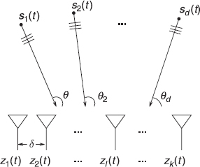
Figure 2.1 A uniform linear array (ULA) of k sensors with sensor displacement δ receiving plane waves from d far-field point sources.
where ω = 2π(δ/λ) sin (θ) depends on the signal wavelength λ, the DOA θ of the signal with respect to broadside, and the sensor spacing δ. The source signal vector s is modeled as either deterministic or random, depending on the application.
In blind signal separation (BSS) based on independent component analysis (ICA), both the mixing system A and the sources s are unknown. The goal in ICA is to solve the mixing matrix and consequently to separate the sources from their mixtures exploiting only the assumption that sources are mutually statistically independent. In this chapter, we consider the noiseless ICA model.
Common assumptions imposed on the signal model (2.1) are as follows:
ASSUMPTION (A1) noise n and/or source s possess circularly symmetric distributions.
In addition, in the process of deriving optimal array processors, the distribution of the noise n is assumed to be known also, the conventional assumption being that
ASSUMPTION (A2) noise n possesses circular complex Gaussian distribution.
Furthermore, if s is modelled as stochastic, then s and n are both assumed to be independent with circular complex Gaussian distribution, and consequently, sensor output z also has k-variate circular complex Gaussian distribution.
In this chapter, we consider the cases where assumptions (A1) and (A2) do not hold. Hence we introduce methods for array processing and ICA that work well at circular and noncircular distributions and when the conventional assumption of normality is not valid. Signal processing examples on beamforming, subspace-based DOA estimation and source-signal separation are provided. Moreover, tests for detecting noncircularity of the data are introduced and the distributions of the test statistics are established as well. Such a test statistic can be used as a guide in choosing the appropriate array processor. For example, if the test rejects the null hypothesis of circularity, it is often wiser to choose a method that explicitly exploits the noncircularity property instead of a method that does not. For example, the generalized uncorrelating transform (GUT) method [47] that is explicitly designed for blind separation of non-circular sources has, in general, better performance in such cases than a method that does not exploit the noncircularity aspect of the sources. Uncertainties related to system matrix, for example, departures from assumed sensor array geometry and related robust estimation procedures are not considered in this chapter.
2.1.2 Outline of the Chapter
This chapter is organized as follows. First, key statistics that are used in describing properties of complex-valued random vectors are presented in Section 2.2. Essential statistics used in this chapter in the characterization of complex random vectors are the circular symmetry, covariance matrix, pseudo-covariance matrix, the strong-uncorrelating transform and the circularity coefficients. The information contained in these statistics can be exploited in designing optimal array processors. In Section 2.3, the class of complex elliptically symmetric (CES) distributions [46] are reviewed. CES distributions constitute a flexible, broad class of distributions that can model both circular/noncircular and heavy-/light-tailed complex random phenomena. It includes the commonly used circular complex normal (CN) distribution as a special case. We also introduce an adjusted generalized likelihood ratio test (GLRT) that can be used for testing circularity when sampling from CES distributions with finite fourth-order moments [40]. This test statistic is shown to be a function of circularity coefficients.
In Section 2.4, tools to compare statistical robustness and statistical efficiency of the estimators are discussed. Special emphasis is put on the concept of influence function (IF) of a statistical functional. IF describes the qualitative robustness of an estimator. Intuitively, qualitative robustness means that the impact of errors to the performance of the estimator is bounded and small changes in the data cause only small changes in the estimates. More explicitly IF measures the sensitivity of the functional to small amounts of contamination in the distribution. It can also be used to calculate the asymptotic covariance structure of the estimator. In Section 2.5, the important concepts of (spatial) scatter matrix and (spatial) pseudo-scatter matrix are defined and examples of such matrix functionals are given. These matrices will be used in developing robust array processors and blind separation techniques that work reliably for both circular/noncircular and Gaussian/non-Gaussian environments. Special emphasis is put on one particularly important class of scatter matrices, called the M-estimators of scatter, that generalize the ML-estimators of scatter matrix parameters of circular CES distributions. Then, in Section 2.6, it is demonstrated how scatter and pseudo-scatter matrices can be used in designing robust beamforming and subspace based DOA estimation methods. Also, a subspace DOA estimation method [13] designed for noncircular sources is discussed. In Section 2.7, we derive the IF of the conventional minimum variance distortionless response (MVDR) beamformer and compare it with the IF of MVDR beamformer employing a robust M-estimator of scatter in place of the conventional covariance matrix. The derived IF of a conventional MVDR beamformer reveals its vulnerability to outliers. IF is further used to compute the asymptotic variances and statistical efficiencies of the MVDR beamformers. MVDR beamformers based on robust M-estimator are shown to be robust (i.e., insensitive to outliers and impulsive noise) without loosing much efficiency (accuracy) under the conventional assumption of normality. Section 2.8 considers the ICA model: we focus on Diagonalization Of Generalized covariance MAtrices (DOGMA) [49] and GUT [47] methods and illustrate how these methods are robust in face of outliers, and also fast to compute.
Notation Symbol | · | denotes the matrix determinant or modulus (i.e. ![]() ) when its argument is a complex scalar, =d reads ‘has the same distribution as’ and →L means convergence in distribution or in law. Recall that every nonzero complex number has a unique (polar) representation, z = |z|ejθ, where −π ≤ θ < π is called the argument of z, denoted θ = arg (z). Complex matrix
) when its argument is a complex scalar, =d reads ‘has the same distribution as’ and →L means convergence in distribution or in law. Recall that every nonzero complex number has a unique (polar) representation, z = |z|ejθ, where −π ≤ θ < π is called the argument of z, denoted θ = arg (z). Complex matrix ![]() is Hermitian if GH = G, symmetric if GT = G and unitary if GHG = I, where I denotes the identity matrix. By PDH(k) and CS(k) we denote the set of k × k positive definite hermitian and complex symmetric matrices, respectively. Recall that all the eigenvalues of PDH(k) matrix are real and positive. If G is a k × k diagonal matrix with diagonal elements g1 …, gk, then we write G = diag(gi).
is Hermitian if GH = G, symmetric if GT = G and unitary if GHG = I, where I denotes the identity matrix. By PDH(k) and CS(k) we denote the set of k × k positive definite hermitian and complex symmetric matrices, respectively. Recall that all the eigenvalues of PDH(k) matrix are real and positive. If G is a k × k diagonal matrix with diagonal elements g1 …, gk, then we write G = diag(gi).
2.2 STATISTICAL CHARACTERIZATION OF COMPLEX RANDOM VECTORS
2.2.1 Complex Random Variables
A complex random variable (rva) z = x + jy is comprised of a pair of real rvas ![]() and
and ![]() The distribution of z is identified with the joint (real bivariate) distribution of real rvas x and y
The distribution of z is identified with the joint (real bivariate) distribution of real rvas x and y
![]()
In a similar manner, the probability density function (pdf) of z = x + jy is identified with the joint pdf f(x, y) of x and y, so f(z) ≡ f(x, y). It is worth pointing out that in some applications (e.g., for optimization purposes [6]) it is preferable to write the pdf f(z) in the form f(z, z*) that separates z and its conjugate z* as if they were independent variates. The mean of z is defined as E[z] = E[x] + jE[y]. For simplicity of presentation, we assume that E[z] = 0.
Characteristics of a complex rva can be described via symmetry properties of its distribution. The most commonly made symmetry assumption in the statistical signal processing literature is that of circular symmetry. See for example [50]. Complex rva z is said to be circular or, to have a circularly symmetric distribution, if
![]()
A circular rva z, in general, does not necessarily possess a density. However, if it does, then its pdf f(z) satisfies
![]()
The property (2.2) can be shown to hold if, and only if, f(z) = f(x, y) is a function of |z|2 = x2 + y2, that is, f(z) = cg(|z|2) for some nonnegative function g(·) and normalizing constant c. Hence the regions of constant contours are circles in the complex plane, thus justifying the name for this class of distributions. rva z is said to be symmetric, or to have a symmetric distribution, if z = d −z. Naturally, circular symmetry implies symmetry.
Characteristics of a complex rva z can also be described via its moments, for example, via its second-order moments. The variance σ2 = σ2(z) > 0 of z is defined as
![]()
Note that variance does not bear any information about the correlation between the real and the imaginary part of z, but this information can be retrieved from pseudo-variance ![]() of z, defined as
of z, defined as
![]()
Note that E[xy] = Im[τ(z)]/2. The complex covariance between complex rvas z and w is defined as
![]()
Thus, σ2(z) = cov(z, z) and τ(z) = cov(z, z*). If z is circular, then τ(z) = 0. Hence a rva z with τ(z) = 0 is called second order circular. Naturally if z or w are (or both z and w are) circular and z ≠ w, then cov(z, w) = 0 as well.
Circularity quotient [41] ![]() of a rva z (with finite variance) is defined as the quotient between the pseudo-variance and the variance
of a rva z (with finite variance) is defined as the quotient between the pseudo-variance and the variance

Thus we can describe ![]() as a measure of correlation between rva z and its conjugate z*. The modulus
as a measure of correlation between rva z and its conjugate z*. The modulus
![]()
is referred to as the circularity coefficient [22, 41] of z. If the rva z is circular, then τ(z) = 0, and consequently λ(z) = 0. Circularity coefficient measures the “amount of circularity” of zero mean rva z = x + jy in that
![]()
Note that λ(z) = 1 if z is purely real-valued such as a BPSK modulated communication signal, or, if the signal lie on a line in the scatter plot (also called constellation or I/Q diagram) as is the case for BPSK, amplitude-shift keying (ASK), amplitude modulation (AM), or PAM-modulated communications signals. Hence a scatter plot of a rvas distrubuted as z with λ = 1 (resp. λ = 0) looks the “least circular” (resp. “most circular”) in the complex plane as measured by its second-order moments. Note that λ is invariant under invertible linear transform ![]() , that is, λ(z) = λ(s). It is worth pointing out that circularity coefficient equals the squared eccentricity of the ellipse defined by the real covariance matrix of the composite real random vector (RV) v = (x, y)T formed by stacking the real and imaginary part of z = x + jy, that is,
, that is, λ(z) = λ(s). It is worth pointing out that circularity coefficient equals the squared eccentricity of the ellipse defined by the real covariance matrix of the composite real random vector (RV) v = (x, y)T formed by stacking the real and imaginary part of z = x + jy, that is,
![]()
where l1 ≥ l2 are the ordered eigenvalues of the 2 × 2 real covariance matrix E[vvT] of v; see [41]. From this formula we observe that λ(z) = 0 if l1 = l2 (i.e., ellipse is a sphere) and λ(z) = 1 if l2 = 0 (i.e., when the ellipse is elongated to a line).
Kurtosis ![]() of z, is defined as
of z, is defined as
![]()
where
![]()
Kurtosis κ(z) describes “peakedness” of the density in that (a) κ = 0 if z is a rva from CN distribution, (b) κ > 0 if it has heavy-tailed (“super-Gaussian”) CES distribution, and (c) κ < 0 if it has light-tailed (“sub-Gaussian”) CES distribution [42]. Similar to the real case, kurtosis κ is defined via complex cumulants. If z is second-order circular, then κ(z) = κ0(z) since λ(z) = 0. Therefore we shall call κ0(z) as the circular kurtosis of z.
2.2.2 Complex Random Vectors
The definitions of Section 2.2.1 can be generalized for complex RVs. A complex RV
![]()
is comprised of a pair of real RVs ![]() and
and ![]() . The distribution of z is identified with the joint real 2k-variate distribution of real RVs x and y. Hence the pdf of z = x + jy is simply the joint pdf f(x, y) of x and y (given it exists), so f(z) ≡ f(x, y). The mean of z is defined as E[z] = E[x] + jE[y]. For simplicity of presentation, we again assume that E[z] = 0. We assume that RV z is non-degenerate in any subspace of
. The distribution of z is identified with the joint real 2k-variate distribution of real RVs x and y. Hence the pdf of z = x + jy is simply the joint pdf f(x, y) of x and y (given it exists), so f(z) ≡ f(x, y). The mean of z is defined as E[z] = E[x] + jE[y]. For simplicity of presentation, we again assume that E[z] = 0. We assume that RV z is non-degenerate in any subspace of ![]() .
.
Similar to the scalar case, random vector z is said to be circular if z = d ejθz for all ![]() . Naturally, the pdf f(z) of a circular RV satisfies f(ejθz) = f(z) for all
. Naturally, the pdf f(z) of a circular RV satisfies f(ejθz) = f(z) for all ![]() In the vector case, however, the term “circular” is a bit misleading since for k ≥ 2, it does not imply that the regions of constant contours are spheres in complex Euclidean k-space.
In the vector case, however, the term “circular” is a bit misleading since for k ≥ 2, it does not imply that the regions of constant contours are spheres in complex Euclidean k-space.
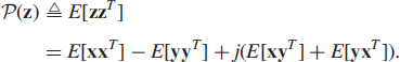
Properties of a complex RV z can be described via its second-order moments. A complete second-order description of complex RV z is given by its covariance matrix ![]() , defined as
, defined as

and the pseudo-covariance matrix [38] ![]() , defined as
, defined as
The pseudo-covariance matrix is also called relation matrix in [50] or complementary covariance matrix in [53]. Random vector z is said to be second-order circular [50] or proper [38] if ![]() , or equivalently, if
, or equivalently, if
![]()
The assumption (2.6) on the covariance structure of the real part x and imaginary part y of z is crucial in writing joint pdf f(x, y) of x and y with real 2k-variate normal distribution into a complex form that is similar to the real case; see [24, 29, 61] and Section 2.3.
There can be several different ways to extend the concept of circularity quotient to the vector case. For example, since the circularity quotient can be written as ![]() , one possible extension is
, one possible extension is
![]()
referred to as the circularity matrix of z. Furthermore, since the circularity coefficient λ(z) is the absolute value of ![]() , that is,
, that is, ![]() , one possible way to extend this concept to the vector case, is to call the square-roots of the eigenvalues of the matrix
, one possible way to extend this concept to the vector case, is to call the square-roots of the eigenvalues of the matrix
![]()
as the circularity coefficients of z. The eigenvalues of ![]() are real-valued and take values on the interval [0, 1]; see Theorem 2 of [47]. Hence, also in this sense, the square-roots of the eigenvalues are valid extensions of the circularity coefficient λ(z) ∈ [0, 1]. Let λi = λi(z) ∈ [0, 1], i = 1, …, k denote the square-roots of the eigenvalues of the matrix
are real-valued and take values on the interval [0, 1]; see Theorem 2 of [47]. Hence, also in this sense, the square-roots of the eigenvalues are valid extensions of the circularity coefficient λ(z) ∈ [0, 1]. Let λi = λi(z) ∈ [0, 1], i = 1, …, k denote the square-roots of the eigenvalues of the matrix ![]() . In deference to [22], we shall call λi (i = 1, …, k) the ith circularity coefficients of z and we write Λ = Λ(z) = diag(λi) for the k × k matrix of circularity coefficients. In [54], it has been shown that circularity coefficients are the canonical correlations between z and its conjugate z*. It is easy to show that circularity coefficients are singular values of the symmetric matrix
. In deference to [22], we shall call λi (i = 1, …, k) the ith circularity coefficients of z and we write Λ = Λ(z) = diag(λi) for the k × k matrix of circularity coefficients. In [54], it has been shown that circularity coefficients are the canonical correlations between z and its conjugate z*. It is easy to show that circularity coefficients are singular values of the symmetric matrix ![]() (called the coherence matrix in [54]), where B(z) is any square-root matrix of
(called the coherence matrix in [54]), where B(z) is any square-root matrix of ![]() (i.e.,
(i.e., ![]() This means that there exists a unitary matrix U such that symmetric matrix K(z) has a special form of singular value decomposition (SVD), called Takagi factorization, such that K(z) = UΛUT. Thus, if we now define matrix
This means that there exists a unitary matrix U such that symmetric matrix K(z) has a special form of singular value decomposition (SVD), called Takagi factorization, such that K(z) = UΛUT. Thus, if we now define matrix ![]() as W = BHU, where B and U are defined as above, then we observe that the transformed data s = WHz satisfies
as W = BHU, where B and U are defined as above, then we observe that the transformed data s = WHz satisfies
![]()
that is, transformed RV s has (strongly-)uncorrelated components. Hence the matrix W is called the strong-uncorrelating transform (SUT) [21, 22].
Note that
![]()
As in the univariate case, circularity coefficients are invariant under the group of invertible linear transformations {![]() nonsingular }, that is, λi(z) = λi(s). Observe that the set of circularity coefficients {λi(z), i = 1, …, k} of the RV z does not necessarily equal the set of circularity coefficient of the variables {λ(zi), i = 1, …, k} although in some cases (for example, when the components z1, …, zk of z are mutually statistically independent) they can coincide.
nonsingular }, that is, λi(z) = λi(s). Observe that the set of circularity coefficients {λi(z), i = 1, …, k} of the RV z does not necessarily equal the set of circularity coefficient of the variables {λ(zi), i = 1, …, k} although in some cases (for example, when the components z1, …, zk of z are mutually statistically independent) they can coincide.
2.3 COMPLEX ELLIPTICALLY SYMMETRIC (CES) DISTRIBUTIONS
Random vector z of ![]() has k-variate circular CN distribution if its real and imaginary part x and y have 2k-variate real normal distribution and a 2k × 2k real covariance matrix with a special form (2.6), that is,
has k-variate circular CN distribution if its real and imaginary part x and y have 2k-variate real normal distribution and a 2k × 2k real covariance matrix with a special form (2.6), that is, ![]() . Since the introduction of the circular CN distribution in [24, 61], the assumption (2.6) seems to be commonly thought of as essential—although it was based on application specific reasoning—in writing the joint pdf f(x, y) of x and y into a natural complex form f(z). In fact, the prefix “circular” is often dropped when referring to circular CN distribution, as it has due time become the commonly accepted complex normal distribution. However, rather recently, in [51, 57], an intuitive expression for the joint density of normal RVs x and y was derived without the unnecessary second-order circularity assumption (2.6) on their covariances. The pdf of z with CN distribution is uniquely parametrized by the covariance matrix
. Since the introduction of the circular CN distribution in [24, 61], the assumption (2.6) seems to be commonly thought of as essential—although it was based on application specific reasoning—in writing the joint pdf f(x, y) of x and y into a natural complex form f(z). In fact, the prefix “circular” is often dropped when referring to circular CN distribution, as it has due time become the commonly accepted complex normal distribution. However, rather recently, in [51, 57], an intuitive expression for the joint density of normal RVs x and y was derived without the unnecessary second-order circularity assumption (2.6) on their covariances. The pdf of z with CN distribution is uniquely parametrized by the covariance matrix ![]() and pseudo-covariance matrix
and pseudo-covariance matrix ![]() , the case of vanishing pseudo-covariance matrix,
, the case of vanishing pseudo-covariance matrix, ![]() , thus indicating the (sub)class of circular CN distributions.
, thus indicating the (sub)class of circular CN distributions.
There are many ways to represent complex random vectors and their probability distributions. The representation exploited in the seminal works of [51, 57] to derive the results is the so-called augmented signal model, where a 2k-variate complex-valued augmented vector
![]()
is formed by stacking the complex vector and its complex conjugate z*. This form is also used in many different applications. The augmentation may also be performed by considering the composite real-valued vectors (xT, yT)T of ![]() . These two augmented models are related via invertible linear transform
. These two augmented models are related via invertible linear transform
![]()
The identity (2.8) can then be exploited as in [51] (resp. [46]) in writing the joint pdf of x and y with 2k-variate real normal (resp. real elliptically symmetric) distribution into a complex form.
2.3.1 Definition
Definition 1 Random vector ![]() is said to have a (centered) CES distribution with parameters Σ ∈ PDH(k) and Ω ∈ CS(k) if its pdf is of the form
is said to have a (centered) CES distribution with parameters Σ ∈ PDH(k) and Ω ∈ CS(k) if its pdf is of the form
![]()
where
![]()
and Δ(z|Γ) is a quadratic form
![]()
and g:[0, ∞) → [0, ∞) is a fixed function, called the density generator, independent of Σ and Ω and ck,g is a normalizing constant. We shall write ![]()
In (2.9), ck,g is defined as ![]() , where
, where ![]() is the surface area of unit complex k-sphere
is the surface area of unit complex k-sphere ![]() and
and

Naturally, ck,g could be absorbed into the function g, but with this notation g can be independent of the dimension k. CES distributions can also be defined more generally (without making the assuption that the probability density function exists) via their characteristic function. The functional form of the density generator g(·) uniquely distinguishes different CES distributions from another. In fact, any nonnegative function g(·) that satisfies μk,g < ∞ is a valid density generator.
The covariance matrix and pseudo-covariance matrix of z ~ FΣ,Ω (if they exist) are proportional to parameters Σ and Ω, namely
![]()
where the positive real-valued scalar factor σC is defined as
![]()
where the positive real rva δ has density
![]()
Hence, the covariance matrix of FΣ,Ω exists if, and only if, E(δ) < ∞, that is, ![]() . Write
. Write
![]()
Then CEk(Σ, Ω, g) with ![]() indicates the subclass of CES distributions with finite moments of order
indicates the subclass of CES distributions with finite moments of order ![]() .
.
Note that the pdf f(z|Σ, Ω) can also be parameterized via matrices [46]

in which case Δ(z|Γ) = zHS−1z − Re(zHS−1RTz*) and |Γ| = |S|2|I − RR*|−1. If ![]() (i.e., the covariance matrix exists), then R is equal to circularity matrix
(i.e., the covariance matrix exists), then R is equal to circularity matrix ![]() defined in (2.7) then since the covariance matrix and pseudo-covariance matrix at FΣ,Ω are proportional to parameters Σ and Ω by (2.11). However, R is a well defined parameter also in the case that the covariance matrix does not exist.
defined in (2.7) then since the covariance matrix and pseudo-covariance matrix at FΣ,Ω are proportional to parameters Σ and Ω by (2.11). However, R is a well defined parameter also in the case that the covariance matrix does not exist.
Recall that the functional form of the density generator g(·) uniquely distinguishes among different CES distributions. We now give examples of well-known CES distributions defined via their density generator.
![]() EXAMPLE 2.1
EXAMPLE 2.1
The complex normal (CN) distribution, labeled Φk, is obtained with
![]()
which gives ck,g = π−k as the value of the normalizing constant. At Φk-distribution, ![]() , so the parameters Σ and Ω coincide with the covariance matrix and pseudo-covariance matrix of the distribution. Thus we write
, so the parameters Σ and Ω coincide with the covariance matrix and pseudo-covariance matrix of the distribution. Thus we write ![]()
![]() EXAMPLE 2.2
EXAMPLE 2.2
The complex t-distribution with ν degrees of freedom (0 < ν < ∞), labeled Tk,ν, is obtained with
![]()
which gives ![]() as the value of the normalizing constant. The case ν = 1 is called the complex Cauchy distribution, and the limiting case ν → ∞ yields the CN distribution. We shall write z ~ CTk,ν(Σ, Ω). Note that the Tk,ν-distribution possesses a finite covariance matrix for ν > 2, in which case
as the value of the normalizing constant. The case ν = 1 is called the complex Cauchy distribution, and the limiting case ν → ∞ yields the CN distribution. We shall write z ~ CTk,ν(Σ, Ω). Note that the Tk,ν-distribution possesses a finite covariance matrix for ν > 2, in which case ![]() .
.
2.3.2 Circular Case
Definition 2 The subclass of CES distributions with Ω = 0, labeled FΣ = CEk(Σ, g) for short, is called circular CES distributions.
Observe that Ω = 0 implies that Δ(z|Γ) = zHΣ−1z and |Γ| = |Σ|2. Thus the pdf of circular CES distribution takes the form familiar from the real case
![]()
Hence the regions of constant contours are ellipsoids in complex Euclidean k-space. Clearly circular CES distributions belong to the class of circularly symmetric distributions since f(ejθz|Σ) = f(z|Σ) for all ![]() . For example,
. For example, ![]() , labeled
, labeled ![]() for short, is called the circular CN distribution (or, proper CN distribution [38]), the pdf now taking the classical [24, 61] form
for short, is called the circular CN distribution (or, proper CN distribution [38]), the pdf now taking the classical [24, 61] form
![]()
See [33] for a detailed study of circular CES distributions.
2.3.3 Testing the Circularity Assumption
In case the signals or noise are noncircular, we need to take the full second-order statistics into account when deriving or applying signal processing algorithms. Hence, there needs to be a way to detect noncircularity. This may be achieved via hypothesis testing; see [46, 54]. In the following, we will develop a generalized likelihood ratio test (GLRT) for detecting noncircularity and establish some asymptotic properties of the test statistics.
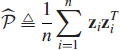
Assume that z1, …, zn is an independent identically distributed (i.i.d.) random sample from a random vector ![]() . Sample covariance matrix (SCM)
. Sample covariance matrix (SCM)
![]()
is then the natural plug-in estimator of the covariance matrix, that is, ![]() is the value of the covariance matrix at the empirical distribution function Fn of the sample. Similarly, sample pseudo-covariance matrix
is the value of the covariance matrix at the empirical distribution function Fn of the sample. Similarly, sample pseudo-covariance matrix
is the plug-in estimator of the pseudo-covariance matrix. In addition, ![]() and
and ![]() are also the ML-estimators when the data is a random sample from
are also the ML-estimators when the data is a random sample from ![]() distribution.
distribution.
In [46] and [54], a GLRT statistic was derived for the the hypothesis
![]()
against the general alternative ![]() . So the purpose is to test the validity of the circularity assumption when sampling from CN distribution. The GRLT decision statistic is
. So the purpose is to test the validity of the circularity assumption when sampling from CN distribution. The GRLT decision statistic is

where ![]() is the likelihood function of the sample and f(· | ·) the pdf of CN distribution. In [46], it was shown that
is the likelihood function of the sample and f(· | ·) the pdf of CN distribution. In [46], it was shown that
![]()
where ![]() is the sample version of the circularity matrix
is the sample version of the circularity matrix ![]() and
and ![]() where
where ![]() is the sample circularity coefficients, that is the square-roots of the eigen-values of
is the sample circularity coefficients, that is the square-roots of the eigen-values of ![]() . This test statistic is invariant (since
. This test statistic is invariant (since ![]() is invariant) under the group of invertible linear transformations. In [40], based on general asymptotic theory of GLR-tests, the following result was shown:
is invariant) under the group of invertible linear transformations. In [40], based on general asymptotic theory of GLR-tests, the following result was shown:
Theorem 1 Under H0, ![]() in distribution, where
in distribution, where ![]() .
.
The test that rejects H0 whenever −n ln ln exceeds the corresponding chi-square (1 − α)th quantile is thus GLRT with asymptotic level α. This test statistic is, however, highly sensitive to violations of the assumption of complex normality. Therefore, in [40], a more general hypothesis was considered also
![]()
Hence the purpose is to test the validity of the circularity assumption when sampling from unspecified (not necessarily normal) CES distributions with finite fourth-order moments. Denotes by κi = κ(zi) the marginal kurtosis of the ith variable zi. Under ![]() , the marginal kurtosis coincide, so
, the marginal kurtosis coincide, so ![]() . In addition, under
. In addition, under ![]() , the circularity coefficient of the marginals vanishes, that is, λ(zi) = 0 for i = 1, …, k, so
, the circularity coefficient of the marginals vanishes, that is, λ(zi) = 0 for i = 1, …, k, so ![]() , where
, where ![]() . Let
. Let ![]() be any consistent estimate of κ. Clearly, a natural estimate of the marginal kurtosis is the average of the sample marginal kurtosis
be any consistent estimate of κ. Clearly, a natural estimate of the marginal kurtosis is the average of the sample marginal kurtosis ![]() , that is,
, that is, ![]() . Then, in [40], an adjusted GLRT-test statistic was shown to be asymptotically robust over the class of CES distributions with finite fourth-order moments.
. Then, in [40], an adjusted GLRT-test statistic was shown to be asymptotically robust over the class of CES distributions with finite fourth-order moments.
Theorem 2 Under ![]() in distribution.
in distribution.
This means that by a slight adjustment, that is, by dividing the GLRT statistic −n log ln by ![]() , we obtain an adjusted test statistic
, we obtain an adjusted test statistic ![]() of circularity that is valid—not just at the CN distribution, but—over the whole class of CES distributions with finite fourth-order moments. Based on the asymptotic distribution, we reject the null hypothesis at (asymptotic) α-level if
of circularity that is valid—not just at the CN distribution, but—over the whole class of CES distributions with finite fourth-order moments. Based on the asymptotic distribution, we reject the null hypothesis at (asymptotic) α-level if ![]() .
.
We now investigate the validity of the ![]() approximation to the finite sample distribution of the adjusted GLRT-test statistic
approximation to the finite sample distribution of the adjusted GLRT-test statistic ![]() at small sample lengths graphically via “chi-square plots”. For this purpose, let
at small sample lengths graphically via “chi-square plots”. For this purpose, let ![]() denote the computed values of the adjusted GLRT-test statistic from N simulated samples of length n and let
denote the computed values of the adjusted GLRT-test statistic from N simulated samples of length n and let ![]() denote the ordered sample, that is, the sample quantiles. Then
denote the ordered sample, that is, the sample quantiles. Then
![]()
are the corresponding theoretical quantiles (where 0.5 in (j − 0.5)/N) is a commonly used continuity correction). Then a plot of the points ![]() should resemble a straight line through the origin having slope 1. Particularly, the theoretical (1 − α)th quantile should be close to the corresponding sample quantile (e.g. α = 0.05). Figure 2.2 depicts such chi-square plots when sampling from circular Tk,ν distribution (with k = 5, ν = 6) using sample lengths n = 100 and n = 500 (i.e.,
should resemble a straight line through the origin having slope 1. Particularly, the theoretical (1 − α)th quantile should be close to the corresponding sample quantile (e.g. α = 0.05). Figure 2.2 depicts such chi-square plots when sampling from circular Tk,ν distribution (with k = 5, ν = 6) using sample lengths n = 100 and n = 500 (i.e., ![]() holds). The number of samples was N = 5000. A very good fit with the straight line is obtained. The dashed vertical (resp. dotted horizontal) line indicates the value for the theoretical (resp. sample) 0.05-upper quantile. The quantiles are almost identical since the lines are crossing approximately on the diagonal. In generating a simulated random sample from circular Tk,ν distribution, we used the property that for independent RV z0 ~ CNk(I) and rva
holds). The number of samples was N = 5000. A very good fit with the straight line is obtained. The dashed vertical (resp. dotted horizontal) line indicates the value for the theoretical (resp. sample) 0.05-upper quantile. The quantiles are almost identical since the lines are crossing approximately on the diagonal. In generating a simulated random sample from circular Tk,ν distribution, we used the property that for independent RV z0 ~ CNk(I) and rva ![]() , the distribution of the composite RV
, the distribution of the composite RV

Figure 2.2 Chi-square plot when sampling from circular Tk,ν distribution (i.e. ![]() ) using sample length n = 100 (a) and n = 500 (b) The number of samples was N = 5000, degrees of freedom (d.f.) parameter was ν = 6 and dimension was k = 5. The dashed vertical (resp. dotted horizontal) line indicate the value for the theoretical (resp. sample) 0.05-upper quantile.
) using sample length n = 100 (a) and n = 500 (b) The number of samples was N = 5000, degrees of freedom (d.f.) parameter was ν = 6 and dimension was k = 5. The dashed vertical (resp. dotted horizontal) line indicate the value for the theoretical (resp. sample) 0.05-upper quantile.
![]()
follows circular Tk,ν distribution with Σ = I, and, z′ = Gz has circular Tk,ν distribution with Σ = GGH for any nonsingular ![]() .
.
If it is not known a priori whether the source signals are circular or noncircular, the decision (accept/reject) of GLRT can be used to guide the selection of the optimal array processor for further processing of the data since optimal array processors are often different for circular and noncircular cases.
We now investigate the performance of the test with a communications example.
![]() EXAMPLE 2.3
EXAMPLE 2.3
Three independent random circular signals—one quadrature phase-shift keying (QPSK) signal, one 16-phase-shift keying (PSK) and one 32-quadrature amplitude modulation (QAM) signal—of equal power ![]() are impinging on an k = 8 element ULA with λ/2 spacing from DOAs − 10°, 15° and 10°. The noise n has circular CN distribution with
are impinging on an k = 8 element ULA with λ/2 spacing from DOAs − 10°, 15° and 10°. The noise n has circular CN distribution with ![]() . The signal to noise ratio (SNR) is 0.05 dB and the number of snapshots is n = 300. Since the noise and the sources are circular, also the marginals zi of the array output z are circular as well, so
. The signal to noise ratio (SNR) is 0.05 dB and the number of snapshots is n = 300. Since the noise and the sources are circular, also the marginals zi of the array output z are circular as well, so ![]() . Then, based on 500 Monte-Carlo trials, the null hypothesis of (second-order) circularity was falsely rejected (type I error) by GLRT test at α = 0.05 level in 5.6 percent of all trials. Hence we observe that the GLRT test performs very well even though the Gaussian data assumption under which the GLRT test statistic ln was derived do not hold exactly. (Since the source RV s is non-Gaussian, the observed array output z = As + n is also non-Gaussian.)
. Then, based on 500 Monte-Carlo trials, the null hypothesis of (second-order) circularity was falsely rejected (type I error) by GLRT test at α = 0.05 level in 5.6 percent of all trials. Hence we observe that the GLRT test performs very well even though the Gaussian data assumption under which the GLRT test statistic ln was derived do not hold exactly. (Since the source RV s is non-Gaussian, the observed array output z = As + n is also non-Gaussian.)
We further investigated the power of the GLRT in detecting noncircularity. For this purpose, we included a fourth source, a BPSK signal, that impinges on the array from DOA 35°. Apart from this additional source signal, the simulation setting is exactly as earlier. Note that the BPSK signal (or any other purely real-valued signal) is noncircular with circularity coefficient λ = 1. Consequently, the array output z is no longer second-order circular. The calculated GLRT-test statistic −n ln ln correctly rejected at the α = 0.05 level the null hypothesis of second-order circularity for all 500 simulated Monte-Carlo trials. Hence, GLRT test was able to detect noncircularity of the snapshot data (in conventional thermal circular Gaussian sensor noise) despite the fact that source signals were non-Gaussian.
2.4 TOOLS TO COMPARE ESTIMATORS
2.4.1 Robustness and Influence Function
In general, robustness in signal processing means insensitivity to departures from underlying assumptions. Robust methods are needed when precise characterization of signal and noise conditions is unrealistic. Typically the deviations from the assumptions occur in the form of outliers, that is, observed data that do not follow the pattern of the majority of the data. Other causes of departure include noise model class selection errors and incorrect assumptions on noise environment. The errors in sensor array and signal models and possible uncertainty in physical signal environment (e.g. propagation) and noise model emphasize the importance of validating all of the assumptions by physical measurements. Commonly many assumptions in multichannel signal processing are made just to make the algorithm derivation easy. For example, by assuming circular complex Gaussian pdfs, the derivation of the algorithms often leads to linear structures because linear transformations of Gaussians are Gaussians.
Robustness can be characterized both quantitatively and qualitatively. Intuitively, quantitative robustness describes how large a proportion of the observed data can be contaminated without causing significant errors (large bias) in the estimates. It is commonly described using the concept of breakdown point. Qualitative robustness on the other hand characterizes whether the influence of highly deviated observations is bounded. Moreover, it describes the smoothness of the estimator in a sense that small changes in the data should cause only small changes in the resulting estimates. We will focus on the qualitative robustness of the estimators using a very powerful tool called the influence function (IF).
Influence function is a versatile tool for studying qualitative robustness (local stability) and large sample properties of estimators, see [26, 27]. Consider the ε-point-mass contamination of the reference distribution F, defined as
![]()
where Δt(z) is a point-mass probability measure that assigns mass 1 to the point t. Then the IF of a statistical functional T at a fixed point t and a given distribution F is defined as
![]()
One may interpret the IF as describing the effect (influence) of an infinitesimal point-mass contamination at a point t on the estimator, standardized by the mass of the contamination. Hence, the IF gives asymptotic bias caused by the contamination. Clearly, the effect on T is desired to be small or at least bounded. See [26] for a more detailed explanation of the influence function.
Let Fn denote the empirical distribution function associated with the data set Zn = {z1, …, zn}. Then a natural plug-in estimator of T(·) is ![]() . If the estimator
. If the estimator ![]() is robust, its theoretical functional T(·) has a bounded and continuous IF. Loosely speaking, the boundedness implies that a small amount of contamination at any point t does not have an arbitrarily large influence on the estimator whereas the continuity implies that the small changes in the data set cause only small changes in the estimator.
is robust, its theoretical functional T(·) has a bounded and continuous IF. Loosely speaking, the boundedness implies that a small amount of contamination at any point t does not have an arbitrarily large influence on the estimator whereas the continuity implies that the small changes in the data set cause only small changes in the estimator.
As the definition of the IF is rather technical, it is intructive to illuminate this concept with the simplest example possible. Let F denote the cumulative distribution function (c.d.f) of a real-valued random variable x symmetric about μ, so F(μ) = 1/2. Then, to estimate the unknown symmetry center μ of F, two commonly used estimates are the sample mean ![]() and the sample median
and the sample median ![]() The expected value and the population median
The expected value and the population median
![]()
(where F−1(q) = inf{x : F(x) ≥ q}) are the statistical functionals corresponding to the sample mean and the median, respectively. Indeed observe for example, that

since PFn (x) = 1/n ∀x = xi, i = 1, …, n. The value of Tave at Fε,t is

Hence
![]()
since Tave(F) = μ (as the expected value of the symmetric c.d.f F is equal to the symmetry center μ of F). The IF for the median Tmed(·) is well-known to be

If the c.d.f. F is the c.d.f. of the standard normal distribution Φ (i.e., μ = 0), then the above IF expressions can be written as
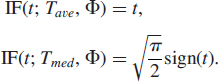
These are depicted in Figure 2.3. The median has bounded IF for all possible values of the contamination t, where as large outlier t can have a large effect on the mean.
![]() EXAMPLE 2.4
EXAMPLE 2.4
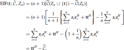
IF of the covariance matrix. Let ![]() be our statistical functional of interest. The value of
be our statistical functional of interest. The value of ![]() at the ε-point-mass distribution is
at the ε-point-mass distribution is

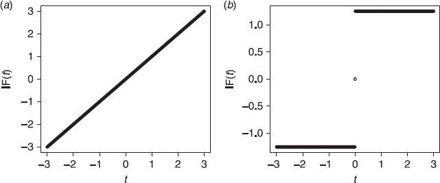
Figure 2.3 The influence functions of the mean Tave(F) = EF[x] (a) and the median Tmed(F) = F−1(1/2) (b) when F is the c.d.f Φ of the standard distribution. The median has bounded influence function for all possible values of the contamination t, where as large outlier t can have a large effect on the mean.
This shows that
![]()
where ![]() denotes the value of the functional
denotes the value of the functional ![]() at the reference distribution F. Thus the IF of
at the reference distribution F. Thus the IF of ![]() is unbounded with respect to standard matrix norms. This means that an infinitesimal point-mass contamination at a point t can have an arbitrarily large influence on the conventional covariance matrix functional, that is, it is not robust.
is unbounded with respect to standard matrix norms. This means that an infinitesimal point-mass contamination at a point t can have an arbitrarily large influence on the conventional covariance matrix functional, that is, it is not robust.
Note however that the IF is an asymptotic concept, characterizing stability of the estimator as n approaches infinity. Corresponding finite sample version is obtained by suppressing the limit in (2.15) and choosing ε = 1/(n + 1) and F = Fn. This yields the empirical influence function (EIF) (also called sensitivity function [26]) of the estimator ![]()
![]()
The EIF thus calculates the standardized effect of an additional observation at t on the estimator. In many cases, the empirical influence function ![]() is a consistent estimator of the corresponding theoretical influence function IF(t; T, F) of the theoretical functional T(·) of the estimator
is a consistent estimator of the corresponding theoretical influence function IF(t; T, F) of the theoretical functional T(·) of the estimator ![]() ; cf. [17, 26].
; cf. [17, 26].
![]() EXAMPLE 2.5
EXAMPLE 2.5
EIF of the sample covariance matrix. If ![]() is the functional of interest, the corresponding plug-in estimator
is the functional of interest, the corresponding plug-in estimator ![]() is naturally the SCM
is naturally the SCM ![]() since
since

Hence we conclude that the EIF of the SCM ![]() is a consistent estimator of the theoretical influence function
is a consistent estimator of the theoretical influence function ![]() (since
(since ![]() is a consistent estimator of the covariance matrix
is a consistent estimator of the covariance matrix ![]() when Zn is a random sample from F).
when Zn is a random sample from F).
2.4.2 Asymptotic Performance of an Estimator
Earlier, we defined the CN distribution ![]() via its density function. More generally we can define the CN distribution via its characteristic function (CF). The CF is a convenient tool for describing probability distributions since it always exists, even when the density function or moments are not well-defined. The CF of CN distribution is [51, 57]
via its density function. More generally we can define the CN distribution via its characteristic function (CF). The CF is a convenient tool for describing probability distributions since it always exists, even when the density function or moments are not well-defined. The CF of CN distribution is [51, 57]
![]()
If the covariance matrix ![]() is nonsingular, then CN possess the density function of Example 2.1. If
is nonsingular, then CN possess the density function of Example 2.1. If ![]() is singular, then the CN distribution is more commonly referred to as singular CN distribution.
is singular, then the CN distribution is more commonly referred to as singular CN distribution.
For a complete second-order description of the limiting distribution of any statistic ![]() we need to provide both the asymptotic covariance and the pseudo-covariance matrix. This may be clarified by noting that the real multivariate central limit theorem (e.g. [4], p. 385) when written into a complex form reads as follows.
we need to provide both the asymptotic covariance and the pseudo-covariance matrix. This may be clarified by noting that the real multivariate central limit theorem (e.g. [4], p. 385) when written into a complex form reads as follows.
Complex Central Limit Theorem (CCLT) Let z1, …, zn ![]() be i.i.d. random vectors from F with mean
be i.i.d. random vectors from F with mean ![]() , finite covariance matrix
, finite covariance matrix ![]() and pseudo-covariance matrix
and pseudo-covariance matrix ![]() , then
, then ![]() .
.
Estimator ![]() of
of ![]() based on i.i.d. random sample z1, …, zn from F has asymptotic CN distribution with asymptotic covariance matrix
based on i.i.d. random sample z1, …, zn from F has asymptotic CN distribution with asymptotic covariance matrix ![]() and asymptotic pseudo-covariance matrix
and asymptotic pseudo-covariance matrix ![]() , if
, if
![]()
If ![]() , then
, then ![]() has asymptotic circular CN distribution. By CCLT, the sample mean
has asymptotic circular CN distribution. By CCLT, the sample mean ![]() has CN distribution with
has CN distribution with ![]() and
and ![]() . Moreover,
. Moreover, ![]() has asymptotic circular CN distribution if, and only if, F is second-order circular.
has asymptotic circular CN distribution if, and only if, F is second-order circular.
Given two competing estimators of the parameter θ, their efficiency of estimating the parameter of interest (at large sample sizes) can be established by comparing the ratio of the matrix traces of their asymptotic covariance matrices at a given reference distribution F, for example. It is very common in statistical signal processing and statistical analysis to define the asymptotic relative efficiency (ARE) of an estimator ![]() as the ratio of the matrix traces of the asymptotic covariance matrices of the estimator and the optimal ML-estimator
as the ratio of the matrix traces of the asymptotic covariance matrices of the estimator and the optimal ML-estimator ![]() . By using such a definition, the ARE of an estimator is always smaller than 1. If the ARE attains the maximum value 1, then the estimator is said to be asymptotically optimal at the reference distribution F. Later in this chapter we conduct such efficiency analysis for the MVDR beamformer based on the conventional sample covariance matrix (SCM) and the M-estimators of scatter.
. By using such a definition, the ARE of an estimator is always smaller than 1. If the ARE attains the maximum value 1, then the estimator is said to be asymptotically optimal at the reference distribution F. Later in this chapter we conduct such efficiency analysis for the MVDR beamformer based on the conventional sample covariance matrix (SCM) and the M-estimators of scatter.
Next we point out that the IF of the functional T(·) can be used to compute the asymptotic covariance matrices of the corresponding estimator ![]() . If a functional T corresponding to an estimator
. If a functional T corresponding to an estimator ![]() is sufficiently regular and z1, …, zn is an i.i.d. random sample from F, one has that [26, 27]
is sufficiently regular and z1, …, zn is an i.i.d. random sample from F, one has that [26, 27]

It turns out that E[IF(z; T, F)] = 0 and, hence by CCLT, ![]() has asymptotic CN distribution
has asymptotic CN distribution
![]()
with
![]()
![]()
Although (2.18) is often true, a rigorous proof may be difficult and beyond the scope of this chapter. However, given the form of the IF, equations (2.19) and (2.20) can be used to calculate an expression for the asymptotic covariance matrix and pseudo-covariance matrix of the estimator ![]() in a heuristic manner.
in a heuristic manner.
2.5 SCATTER AND PSEUDO-SCATTER MATRICES
2.5.1 Background and Motivation
A starting point for many multiantenna transceiver and smart antenna algorithms is the array covariance matrix. For example, many direction-of-arrival (DOA) estimation algorithms such as the classical (delay-and-sum) beamformer and the Capon's MVDR beamformer require the array covariance matrix to measure the power of the beamformer output as a function of angle of arrival or departure. In addition, many high-resolution subspace-based DOA algorithms (such as MUSIC, ESPRIT, minimum norm etc.) compute the noise or signal subspaces from the eigenvectors of the array covariance matrix and exploit the fact that signal subspace eigenvectors and steering vector A matrix span the same subspace. See for example, [32, 55] and Section 2.6 for a overview of beamforming and subspace approaches to DOA estimation.
Since the covariance matrix is unknown, the common practice is to use the SCM ![]() estimated from the snapshot data in place of its true unknown quantity. Although statistical optimality can often be claimed for array processors using the SCM under the normal (Gaussian) data assumption, they suffer from a lack of robustness in the face of outliers, that is, highly deviating observations and signal or noise modeling errors. Furthermore, their efficiency for heavy-tailed non-Gaussian and impulsive noise environments properties are far from optimal. It is well known that if the covariance matrix is estimated in a nonrobust manner, statistics (such as eigenvalues and eigenvectors) based on it are unreliable and far from optimal. In fact, such estimators may completely fail even in the face of only minor departures from the nominal assumptions. A simple and intuitive approach to robustify array processors is then to use robust covariance matrix estimators instead of the conventional nonrobust SCM
estimated from the snapshot data in place of its true unknown quantity. Although statistical optimality can often be claimed for array processors using the SCM under the normal (Gaussian) data assumption, they suffer from a lack of robustness in the face of outliers, that is, highly deviating observations and signal or noise modeling errors. Furthermore, their efficiency for heavy-tailed non-Gaussian and impulsive noise environments properties are far from optimal. It is well known that if the covariance matrix is estimated in a nonrobust manner, statistics (such as eigenvalues and eigenvectors) based on it are unreliable and far from optimal. In fact, such estimators may completely fail even in the face of only minor departures from the nominal assumptions. A simple and intuitive approach to robustify array processors is then to use robust covariance matrix estimators instead of the conventional nonrobust SCM ![]() . This objective leads to the introduction of a more general notion of covariance, called the scatter matrix.
. This objective leads to the introduction of a more general notion of covariance, called the scatter matrix.
As was explained in Section 2.2, the covariance matrix ![]() unambiguously describes relevant correlations between the variables in the case that the distribution F of z is circular symmetric. In the instances that F is noncircular distribution, also the information contained in the pseudo-covariance matrix
unambiguously describes relevant correlations between the variables in the case that the distribution F of z is circular symmetric. In the instances that F is noncircular distribution, also the information contained in the pseudo-covariance matrix ![]() can/should be exploited for example, in the blind estimation of noncircular sources or in the process of recovering the desired signal and cancelling the interferences. Therefore, in the case of noncircularity, an equally important task is robust estimation of the pseudo-covariance matrix. This objective leads to the introduction of a more general notion of pseudo-covariance, called the pseudo-scatter matrix.
can/should be exploited for example, in the blind estimation of noncircular sources or in the process of recovering the desired signal and cancelling the interferences. Therefore, in the case of noncircularity, an equally important task is robust estimation of the pseudo-covariance matrix. This objective leads to the introduction of a more general notion of pseudo-covariance, called the pseudo-scatter matrix.
2.5.2 Definition
Scatter and pseudo-scatter matrix are best described as generalizations of the covariance and pseudo-covariance matrix, respectively.
Definition 3 Let
![]()
denote the nonsingular linear and unitary transformations of ![]() for any nonsingular
for any nonsingular ![]() and unitary
and unitary ![]()
(a) Matrix functional C ∈ PDH(k) is called a scatter matrix (resp. spatial scatter matrix) if C(s) = AC(z)AH (resp. P(v) = UP(z)UH).
(b) Matrix functional P ∈ CS(k) is called a pseudo-scatter matrix (resp. spatial pseudo-scatter matrix) if P(s) = AP(z)AT (resp. P(v) = UP(z)UT).
Spatial (pseudo-)scatter matrix is a broader notion than the (pseudo-)scatter since it requires equivariance only under unitary linear transformations, that is, every (pseudo-)scatter is also a spatial (pseudo-)scatter matrix. Weighted spatial covariance matrix
![]()
and weighted spatial pseudo-covariance matrix
![]()
where φ(·) denotes any real-valued weighting function on [0, ∞), are examples of a spatial scatter and spatial pseudo-scatter matrix (but not of a (pseudo-)scatter matrix), respectively. Using weight φ(x) = x, we obtain matrices called the kurtosis matrix [49] and pseudo-kurtosis matrix [47]
![]()
Using weight φ(x) = x−1, we obtain matrices called the sign covariance matrix [49, 59] and the sign pseudo-covariance matrix [47]
![]()
These matrix functionals have been shown to be useful in blind separation and array signal processing problems. (cf. [8, 47, 49, 59]) and they possess very different statistical (e.g. robustness) properties. Sign covariance and sign pseudo-covariance matrices are highly robust in the face of non-Gaussian noise. The name for these matrices stems from the observation that “spatial sign” vector ![]() (a unit vector pointing towards the direction of z) can be thought of as a generalization of the univariate sign of an observation which also provides information about the direction of the observation with respect to origin but not its magnitude. Robustness derives from the fact that they use only directional information. The use of the sign covariance matrix in high-resolution DOA estimation is briefly decribed later in this chapter.
(a unit vector pointing towards the direction of z) can be thought of as a generalization of the univariate sign of an observation which also provides information about the direction of the observation with respect to origin but not its magnitude. Robustness derives from the fact that they use only directional information. The use of the sign covariance matrix in high-resolution DOA estimation is briefly decribed later in this chapter.
The covariance matrix ![]() and pseudo-covariance matrix
and pseudo-covariance matrix ![]() serve as examples of a scatter and pseudo-scatter matrix, respectively, assuming z has finite second-order moments. Scatter or pseudo-scatter matrices (or spatial equivalents), by their definition, do not necessarily require the assumption of finite second-order moments for its existence and are therefore capable in describing dependencies between complex random variables in more general settings than the covariance and pseudo-covariance matrix.
serve as examples of a scatter and pseudo-scatter matrix, respectively, assuming z has finite second-order moments. Scatter or pseudo-scatter matrices (or spatial equivalents), by their definition, do not necessarily require the assumption of finite second-order moments for its existence and are therefore capable in describing dependencies between complex random variables in more general settings than the covariance and pseudo-covariance matrix.
More general members of the family of scatter and pseudo-scatter matrices are the weighted covariance matrix and weighted pseudo-covariance matrix, defined as

respectively, where φ(·) is any real-valued weighting function on [0, ∞) and C is any scatter matrix, for example, the covariance matrix. Note that the covariance matrix and the pseudo-covariance matrix are obtained with unit weight φ ≡ 1.
An improved idea of the weighted covariance matrices are M-estimators of scatter, reviewed in detail in the next section. M-estimators of scatter constitute a broad class which include for example MLEs of the parameter Σ of circular CES distributions FΣ. Weighted covariance matrix can be thought of as “1-step M-estimator”.
2.5.3 M-estimators of Scatter
One of the first proposals of robust scatter matrix estimators were M-estimators of scatter due to Maronna [37]. Extension of M-estimators for complex-valued data has been introduced and studied in [43–45, 48]. As in the real case they can be defined by generalizing the MLE.
Let z1, …, zn be an i.i.d. sample from a circular CES distribution FΣ = CEk(Σ, g), where n > k (i.e., sample size n is larger than the number of sensors k). The MLE of Σ, is found by minimizing the negative of the log-likelihood function
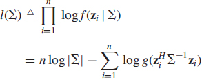
where we have omitted the constant term (the logarithm of the normalizing constant, log [ck,g]) since it does not depend on the unknown parameter Σ. By differentiating l(Σ) with respect to Σ (using complex matrix differentiation rules [6]) shows that the MLE is a solution to estimating equation

where
![]()
is a weight function that depends on the density generator g(·) of the underlying circular CES distribution. For the CN distribution (i.e., when g(δ) = exp (− δ)), we have that φml ≡ 1, which yields the SCM ![]() as the MLE of Σ. The MLE for Tk,ν distribution (cf. Example 2.2), labeled MLT(ν), is obtained with
as the MLE of Σ. The MLE for Tk,ν distribution (cf. Example 2.2), labeled MLT(ν), is obtained with
![]()
Note that MLT(1) is the highly robust estimator corresponding to MLE of Σ for the complex circular Cauchy distribution, and that ![]() as ν → ∞, thus the robustness of MLT(ν) estimators decrease with increasing values of ν.
as ν → ∞, thus the robustness of MLT(ν) estimators decrease with increasing values of ν.
We generalize (2.22), by defining the M-estimator of scatter, denoted by ![]() , as the choice of C ∈ PDH(k) that solves the estimating equation
, as the choice of C ∈ PDH(k) that solves the estimating equation
where φ is any real-valued weight function on [0, ∞). Hence M-estimators constitute a wide class of scatter matrix estimators that include the MLE's for circular CES distributions as important special cases. M-estimators can be calculated by a simple iterative algorithm described later in this section.
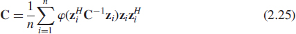
The theoretical (population) counterpart, the M-functional of scatter, denoted by Cφ(z), is defined analogously as the solution of an implicit equation
![]()
Observe that (2.26) reduces to (2.25) when F is the empirical distribution Fn, that is, the solution ![]() of (2.25) is the natural plug-in estimator Cφ(Fn). It is easy to show that the M-functional of scatter is equivariant under invertible linear transformation of the data in the sense required from a scatter matrix. Due to equivariance, Cφ(FΣ) = σφΣ, that is, the M-functional is proportional to the parameter Σ at FΣ, where the positive real-valued scalar factor σφ = σφ(δ) may be found by solving
of (2.25) is the natural plug-in estimator Cφ(Fn). It is easy to show that the M-functional of scatter is equivariant under invertible linear transformation of the data in the sense required from a scatter matrix. Due to equivariance, Cφ(FΣ) = σφΣ, that is, the M-functional is proportional to the parameter Σ at FΣ, where the positive real-valued scalar factor σφ = σφ(δ) may be found by solving
![]()
where δ has density (2.12). Often σφ need to be solved numerically from (2.27) but in some cases an analytic expression can be derived. Since parameter Σ is proportional to underlying covariance matrix ![]() , we conclude that the M-functional of scatter is also proportional to the covariance matrix provided it exists (i.e.,
, we conclude that the M-functional of scatter is also proportional to the covariance matrix provided it exists (i.e., ![]() ). In many applications in sensor array processing, covariance matrix is required only up to a constant scalar (see e.g. Section 2.7), and hence M-functionals can be used to define a robust class of array processors.
). In many applications in sensor array processing, covariance matrix is required only up to a constant scalar (see e.g. Section 2.7), and hence M-functionals can be used to define a robust class of array processors.
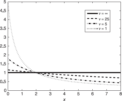
Figure 2.4 φ(X) of MLT(ν) estimators.
By equation (2.25), ![]() can be interpreted as a weighted covariance matrix. Hence, a robust weight function φ should descend to zero. This means that small weights are given to those observations zi that are highly outlying in terms of measure
can be interpreted as a weighted covariance matrix. Hence, a robust weight function φ should descend to zero. This means that small weights are given to those observations zi that are highly outlying in terms of measure ![]() . It downweights highly deviating observations and consequently makes their influence in the error criterion bounded. Note that SCM
. It downweights highly deviating observations and consequently makes their influence in the error criterion bounded. Note that SCM ![]() is an M-estimator that gives unit weight (φ ≡ 1) to all observations. Figure 2.4 plots the weight function (2.24) of MLT(ν) estimators for selected values of ν. Note that weight function (2.24) tends to weight function φ ≡ 1 of the SCM as expected (since Tk,ν tends to Φk distribution when ν → ∞). Thus,
is an M-estimator that gives unit weight (φ ≡ 1) to all observations. Figure 2.4 plots the weight function (2.24) of MLT(ν) estimators for selected values of ν. Note that weight function (2.24) tends to weight function φ ≡ 1 of the SCM as expected (since Tk,ν tends to Φk distribution when ν → ∞). Thus, ![]() for large values of ν.
for large values of ν.
Some examples of M-estimators are given next; See [43–45, 48] for more detailed descriptions of these estimators.
![]() EXAMPLE 2.6
EXAMPLE 2.6
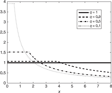
Huber's M-estimator, labeled HUB(q), is defined via weight
![]()
where c is a tuning constant defined so that ![]() for a chosen q(0 < q ≤ 1) and the scaling factor
for a chosen q(0 < q ≤ 1) and the scaling factor ![]() . The choice q = 1 yields φ ≡ 1, that is, HUB(1) correspond to the SCM. In general, low values of q increase robustness but decrease efficiency at the nominal circular CN model. Figure 2.5. depicts weight function of HUB(q) estimators for selected values of q.
. The choice q = 1 yields φ ≡ 1, that is, HUB(1) correspond to the SCM. In general, low values of q increase robustness but decrease efficiency at the nominal circular CN model. Figure 2.5. depicts weight function of HUB(q) estimators for selected values of q.
![]() EXAMPLE 2.7
EXAMPLE 2.7
Tyler's M-estimator of scatter [30, 44] utilizes weight function
![]()
This M-estimator of scatter is also the MLE of the complex angular cental Gaussian distribution [30].
Computation of M-estimators Given any initial estimate ![]() , the iterations
, the iterations

converge to the solution ![]() of (2.25) under some mild regularity conditions. The authors of [27, 31, 37] consider the real case only, but the complex case follows similarly. See also discussions in [44].
of (2.25) under some mild regularity conditions. The authors of [27, 31, 37] consider the real case only, but the complex case follows similarly. See also discussions in [44].
As an example, let the initial estimate be the SCM, that is, ![]() . The first iteration, or the “1-step M-estimator”, is simply a weighted sample covariance matrix
. The first iteration, or the “1-step M-estimator”, is simply a weighted sample covariance matrix
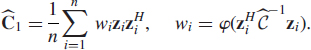
If φ(·) is a robust weighting function, then ![]() is a robustified version of
is a robustified version of ![]() . At the second iteration step, we calculate
. At the second iteration step, we calculate ![]() as a weighted sample covariance matrix using weights
as a weighted sample covariance matrix using weights ![]() and proceed analogously until the iterations
and proceed analogously until the iterations ![]() “converge”, that is,
“converge”, that is, ![]() , where
, where ![]() is a matrix norm and ε is predetermined tolerance level, for example, ε = 0.001. To reduce computation time, one can always stop after m (e.g. m = 4) iterations and take the “m-step M-estimator”
is a matrix norm and ε is predetermined tolerance level, for example, ε = 0.001. To reduce computation time, one can always stop after m (e.g. m = 4) iterations and take the “m-step M-estimator” ![]() as an approximation for the true M-estimator
as an approximation for the true M-estimator ![]() . MATLAB functions to compute MLT(ν), HUB(q) and Tyler's M-estimator of scatter are available at http://wooster.hut.fi/~esollila/MVDR/.
. MATLAB functions to compute MLT(ν), HUB(q) and Tyler's M-estimator of scatter are available at http://wooster.hut.fi/~esollila/MVDR/.
2.6 ARRAY PROCESSING EXAMPLES
Most array processing techniques and smart antenna algorithms employ the SCM ![]() . In the case of heavy-tailed signals or noise, it may give poor performance. Hence, robust array processors that perform reliably and are close to optimal in all scenarios are of interest.
. In the case of heavy-tailed signals or noise, it may give poor performance. Hence, robust array processors that perform reliably and are close to optimal in all scenarios are of interest.
2.6.1 Beamformers
Beamforming is among the most important tasks in sensor array processing. Consequently, there exists a vast amount of research papers on beamforming techniques, see [36, 55, 58] for overviews.
Let us first recall the beamforming principles in narrowband applications. In receive beamforming, the beamformer weight vector w linearly transforms the output signal z of array of k sensors to form the beamformer output
![]()
with an aim of enhancing the signal-of-interest (SOI) from look direction (DOA of SOI) ![]() and attenuating undesired signals (interferers) from other directions. The (look direction dependent) beam response or gain is defined as
and attenuating undesired signals (interferers) from other directions. The (look direction dependent) beam response or gain is defined as
![]()
where a(θ) is the array response (steering vector) to DOA θ. The modulus squared |b(θ)|2 as a function of θ is called the beampattern or antenna pattern. Then, beamformer output power
![]()
should provide an indication of the amount of energy coming from the fixed look direction ![]() . Plotting P(θ) as a function of look direction θ is called the spatial spectrum. The d highest peaks of the spatial spectrum correspond to the beamformer DOA estimates.
. Plotting P(θ) as a function of look direction θ is called the spatial spectrum. The d highest peaks of the spatial spectrum correspond to the beamformer DOA estimates.
The beamformer weight vector w is chosen with an aim that it is statistically optimum in some sense. Naturally, different design objectives lead to different beamformer weight vectors. For example, the weight vector for the classic beamformer is
![]()
where ![]() denotes the array response for fixed look direction
denotes the array response for fixed look direction ![]() . The classic Capon's [7] MVDR beamformer chooses w as the minimizer of the output power while constraining the beam response along a specific look direction
. The classic Capon's [7] MVDR beamformer chooses w as the minimizer of the output power while constraining the beam response along a specific look direction ![]() of the SOI to be unity
of the SOI to be unity
![]()
The well-known solution to this constrained optimization problem is

Observe that Capon's beamformer weight vector is data dependent whereas the classic beamformer weight wBF is not, that is, ![]() is a statistical functional as its value depends on the distribution F of z via the covariance matrix
is a statistical functional as its value depends on the distribution F of z via the covariance matrix ![]() . The spectrum (2.28) for the classic and Capon's beamformers can now be written as
. The spectrum (2.28) for the classic and Capon's beamformers can now be written as
![]()
![]()
respectively. (See Section 6 in [55]). Note that MVDR beamformers do not make any assumption on the structure of the covariance matrix (unlike the subspace-methods of the next section) and hence can be considered as a “nonparametric method” [55].
In practice, the DOA estimates for the classic and Capon's beamformer are calculated as the d highest peaks in the estimated spectrums ![]() and
and ![]() , where the true unknown covariance matrix
, where the true unknown covariance matrix ![]() is replaced by its conventional estimate, the SCM
is replaced by its conventional estimate, the SCM ![]() . An intuitive approach in obtaining robust beamformer DOA estimates is to use robust estimators instead of the SCM in (2.30) and (2.31), for example, the M-estimators of scatter. Rigorous statistical robustness and efficiency analysis of MVDR beamformers based on M-estimators of scatter is presented in Section 2.7.
. An intuitive approach in obtaining robust beamformer DOA estimates is to use robust estimators instead of the SCM in (2.30) and (2.31), for example, the M-estimators of scatter. Rigorous statistical robustness and efficiency analysis of MVDR beamformers based on M-estimators of scatter is presented in Section 2.7.
2.6.2 Subspace Methods
A standard assumption imposed by subspace methods is that the additive noise n is spatially white, that is ![]() . We would like to stress that this assumption does not imply that n is second-order circular, that is, n can have non-vanishing pseudo-covariance matrix. Since source s and noise n are assumed to be mutually statistically independent, the array covariance matrix of the array output z = As + n can be written in the form
. We would like to stress that this assumption does not imply that n is second-order circular, that is, n can have non-vanishing pseudo-covariance matrix. Since source s and noise n are assumed to be mutually statistically independent, the array covariance matrix of the array output z = As + n can be written in the form
![]()
where A = A(θ) is the array response matrix parametrized by the vector of DOAs θ = (θ1, …, θd)T. Low rank signal model is assumed where d < k. Due to the structure (2.32), the k − d smallest eigenvalues of ![]() are equal to σ2 and the corresponding eigenvectors ed+1, …, ek are orthogonal to the columns of A. These eigenvectors span the noise subspace and the eigenvectors e1, …, ed corresponding to d largest eigenvalues span the signal subspace (the column space of A).
are equal to σ2 and the corresponding eigenvectors ed+1, …, ek are orthogonal to the columns of A. These eigenvectors span the noise subspace and the eigenvectors e1, …, ed corresponding to d largest eigenvalues span the signal subspace (the column space of A).
The subspace DOA estimation methods are based on different properties of the signal/noise subspaces. Some subspace methods also impose additional assumptions on the array geometry (e.g. ESPRIT). Essentially, subspace methods need to solve the following two problems.
- Find an estimate
 of the signal subspace Es = (e1 … ed) and/or estimate
  of the noise subspace En = (ed+1 … ek).
 - Find estimate
 of the DOAs which best optimizes the selected error criterion, for example, find such that distance between subspace
  and the estimated subspace
  is minimal in some sense.
Commonly, the subspace methods differ only in how they approach problem 2 since the estimates of signal and noise subspaces are calculated from the eigenvectors of the conventional, nonrobust SCM ![]() . Solving problem 1 reliably, however, is much more crucial since no matter how clever criterion is used or how distances between subspaces are measured in problem 2, the DOA estimates will be unreliable if the estimates of the subspaces are unreliable. In other words, accuracy and efficiency of the subspace method depends largely on the accuracy and efficiency of the estimates of the noise or signal subspaces. Again, to obtain robust subspace methods it is sensible to use estimates of noise or signal subspaces based on eigenvectors of the M-estimators of scatter for example.
. Solving problem 1 reliably, however, is much more crucial since no matter how clever criterion is used or how distances between subspaces are measured in problem 2, the DOA estimates will be unreliable if the estimates of the subspaces are unreliable. In other words, accuracy and efficiency of the subspace method depends largely on the accuracy and efficiency of the estimates of the noise or signal subspaces. Again, to obtain robust subspace methods it is sensible to use estimates of noise or signal subspaces based on eigenvectors of the M-estimators of scatter for example.
The classical MUSIC method is based on the orthogonality of the signal and noise subspace and the fact that A and Es span the same subspace. Because of the orthogonality of the signal and noise subspace, ![]() , or equivalently
, or equivalently
![]()
at the DOAs θ1, …, θd. Then, the MUSIC methods find DOA estimates as the d highest peaks of the MUSIC spectrum
![]()
Clearly, if noise subspace ![]() is unreliably estimated (e.g. via eigenvectors of the SCM when the noise is non-Gaussian or impulsive), then the obtained MUSIC DOA estimators are unreliable. For robust estimation of noise subspace one may use for example, eigenvectors of M-estimators of scatter, or, eigenvectors of the sample plug-in estimate
is unreliably estimated (e.g. via eigenvectors of the SCM when the noise is non-Gaussian or impulsive), then the obtained MUSIC DOA estimators are unreliable. For robust estimation of noise subspace one may use for example, eigenvectors of M-estimators of scatter, or, eigenvectors of the sample plug-in estimate
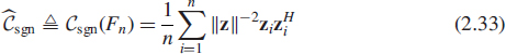
of the sign covariance matrix ![]() as in [59].
as in [59].
A weighted signal subspace fitting (SSF) approach, for example, finds DOAs via criterion function
![]()
where ![]() is a projection matrix onto the noise subspace and Y is some weighting matrix. The estimated optimal weighting matrix
is a projection matrix onto the noise subspace and Y is some weighting matrix. The estimated optimal weighting matrix ![]() is a diagonal matrix, whose diagonal elements are certain functions of the estimated eigenvalues of the covariance matrix
is a diagonal matrix, whose diagonal elements are certain functions of the estimated eigenvalues of the covariance matrix ![]() . Hence, reliable and accurate estimation of DOAs via weighted SSF approach requires robust estimation of the signal subspace Es and eigenvalues of the covariance matrix. These can be obtained, for example, using eigenvectors and eigenvalues of robust M-estimators instead of the SCM.
. Hence, reliable and accurate estimation of DOAs via weighted SSF approach requires robust estimation of the signal subspace Es and eigenvalues of the covariance matrix. These can be obtained, for example, using eigenvectors and eigenvalues of robust M-estimators instead of the SCM.
![]() EXAMPLE 2.8
EXAMPLE 2.8
Four independent random signals, QPSK, 16-PSK, 32-QAM and BPSK signal of equal power ![]() , are impinging on a k = 8 element ULA with λ/2 spacing from DOAs −10°, 15°, 10° and 35°. The simulation setting is as in Example 2.3, except that now we consider two different noise environments. In the first setting, noise n has circular Gaussian distribution
, are impinging on a k = 8 element ULA with λ/2 spacing from DOAs −10°, 15°, 10° and 35°. The simulation setting is as in Example 2.3, except that now we consider two different noise environments. In the first setting, noise n has circular Gaussian distribution ![]() , and in the second setting noise has circular Cauchy distribution
, and in the second setting noise has circular Cauchy distribution ![]() . Note that the Cauchy distribution does not have finite variance and
. Note that the Cauchy distribution does not have finite variance and ![]() is the scale parameter of the distribution. In both simulation settings, the signal to noise ratio (SNR) is
is the scale parameter of the distribution. In both simulation settings, the signal to noise ratio (SNR) is ![]() and the number of snapshots is n = 300. The number of signals (d = 4) is assumed to be known a priori. We then estimated the noise subspace
and the number of snapshots is n = 300. The number of signals (d = 4) is assumed to be known a priori. We then estimated the noise subspace ![]() from eigenvectors of the SCM
from eigenvectors of the SCM ![]() , sample sign covariance matrix (2.33) and MLT(1) estimator. Typical MUSIC spectrums associated with different estimators are shown in Figure 2.6 for both the Gaussian and Cauchy noise settings. All the estimators are able to resolve the four sources correctly in the Gaussian noise case: in fact, the differences in the spectrums are very minor, that is, they provide essentially the same DOA estimates. In the Cauchy noise case, however, MUSIC based on the classical sample estimator
, sample sign covariance matrix (2.33) and MLT(1) estimator. Typical MUSIC spectrums associated with different estimators are shown in Figure 2.6 for both the Gaussian and Cauchy noise settings. All the estimators are able to resolve the four sources correctly in the Gaussian noise case: in fact, the differences in the spectrums are very minor, that is, they provide essentially the same DOA estimates. In the Cauchy noise case, however, MUSIC based on the classical sample estimator ![]() is not able to resolve the sources. The robust estimators, the sign covariance matrix and the MLT(1) estimator, however, yield reliable estimates of the DOAs. Based on the sharpness of the peaks, the MLT(1) estimator is performing better than the sample sign covariance matrix
is not able to resolve the sources. The robust estimators, the sign covariance matrix and the MLT(1) estimator, however, yield reliable estimates of the DOAs. Based on the sharpness of the peaks, the MLT(1) estimator is performing better than the sample sign covariance matrix ![]() .
.

Figure 2.6 MUSIC spectrums when the noise subspace is estimated using SCM ![]() (a), sample sign covariance matrix (b) and MLT(1) estimator (c) in circular Gaussian (first column) and Cauchy (second column) noise. Sources are independent random QPSK, 16-PSK, 32-QAM and BPSK signals that arrive at 8-element ULA from DOAs −10°, 15°, 10° and 35°.
(a), sample sign covariance matrix (b) and MLT(1) estimator (c) in circular Gaussian (first column) and Cauchy (second column) noise. Sources are independent random QPSK, 16-PSK, 32-QAM and BPSK signals that arrive at 8-element ULA from DOAs −10°, 15°, 10° and 35°.
2.6.3 Estimating the Number of Sources
An equally important problem to DOA estimation is the estimation of the number of sources. The subspace based methods introduced in the previous section usually assume that the number of source signals is known a priori. In practise, the number of sources d is often not known and needs to be estimated from the data. The commonly used minimum description length (MDL)-based information theoretical criterion, obtains the estimate ![]() for the number of signals d as an integer p ∈ (0, 1, …, k − 1) which minimizes the criterion [60]
for the number of signals d as an integer p ∈ (0, 1, …, k − 1) which minimizes the criterion [60]
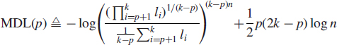
where l1, l2, …, lk denote the (ordered) eigenvalues of the SCM ![]() arranged in descending order. Instead of using the eigenvalues of SCM, it is desirable for purposes of reliable estimation in non-Gaussian noise to employ eigenvalues of some robust estimator of covariance, for example, M-estimator of scatter, instead of the SCM. We demonstrate this via a simulation study.
arranged in descending order. Instead of using the eigenvalues of SCM, it is desirable for purposes of reliable estimation in non-Gaussian noise to employ eigenvalues of some robust estimator of covariance, for example, M-estimator of scatter, instead of the SCM. We demonstrate this via a simulation study.
The ULA contains k = 8 sensors with half a wavelength interelement spacing. Two uncorrelated Gaussian signals with equal power 20 dB from DOAs θ1 = −5° and θ2 = 5° are impinging on the array. The components of the additive noise n are modeled as i.i.d. with complex symmetric α-stable (SαS) distribution [56] with dispersion γ = 1 and values α ranging from α = 1 (complex Cauchy noise) to α = 2 (complex Gaussian noise). Simulation results are based on 500 Monte Carlo runs with n = 300 as the sample size. Figure 2.7 depicts the relative proportion of correct estimation results using MDL criterion, when the eigenvalues are obtained from SCM ![]() and robust MLT(1), HUB(0.9) and HUB(0.5) estimators. The performance of the classic MDL employing the SCM is poor: it is able to estimate the number of signals reliably only for α = 2, that is, the Gaussian case. However, the robust M-estimator is able to estimate the number of sources reliably for large range of α-values. Among the robust M-estimators, MLT(1) has the best performance.
and robust MLT(1), HUB(0.9) and HUB(0.5) estimators. The performance of the classic MDL employing the SCM is poor: it is able to estimate the number of signals reliably only for α = 2, that is, the Gaussian case. However, the robust M-estimator is able to estimate the number of sources reliably for large range of α-values. Among the robust M-estimators, MLT(1) has the best performance.

Figure 2.7 Simulation results for estimation of number of sources using the MDL criterion based on the SCM, HUB(0.9), HUB(0.5) and MLT(1)-estimators. There are d = 2 Gaussian source signals in SαS distributed noise for 1 ≤ α ≤ 2. The number of sensors is k = 8 and number of snapshot is n = 300.
2.6.4 Subspace DOA Estimation for Noncircular Sources
We now describe the Root-MUSIC-like method presented in [13]. As usual, assume that the signal s and noise n in the array model (2.1) are uncorrelated with zeromean. The method further requires the following additional assumptions.
(1) The array is ULA (in order to facilitate using polynomial rooting).
(2) Noise n is second-order circular and spatially white, that is ![]() and
and ![]() .
.
(3) Sources signals si, i = 1, …, d are uncorrelated in the sense that ![]() and
and ![]() .
.
Under these assumptions,
![]()
where as earlier A = A(θ) denotes the array response matrix. Further assume that
(4) ![]() , where Φ = diag(ejϕi).
, where Φ = diag(ejϕi).
Assumption (4) means that the circularity coefficient of the sources are equal to unity, that is, λ(si) = 1 for i = 1, …, d, which by (2.3) implies that transmitted source signal si must be real-valued, such as AM or BPSK modulated signals, or the real part Re(si) of the transmitted signal is a linear function of the imaginary part Im(si). If (1)–(4) hold, then the covariance matrix for the augmented signal vector ![]() is
is
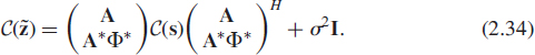
Now by performing eigenvalue decomposition ![]() we may find d dimensional signal subspace and 2k − d dimensional orthogonal noise subspace. Thus Root-MUSIC-like direction finding algorithms can be designed; see [13] for details. By exploiting the noncircularity property we obtain extra degrees of freedom since noncircularity allows resolving more sources than sensors. Again, in the face heavy-tailed noise or outlying observations, a robust estimate of the array covariance matrix
we may find d dimensional signal subspace and 2k − d dimensional orthogonal noise subspace. Thus Root-MUSIC-like direction finding algorithms can be designed; see [13] for details. By exploiting the noncircularity property we obtain extra degrees of freedom since noncircularity allows resolving more sources than sensors. Again, in the face heavy-tailed noise or outlying observations, a robust estimate of the array covariance matrix ![]() and pseudo-covariance matrix
and pseudo-covariance matrix ![]() can be used instead of the conventional estimators,
can be used instead of the conventional estimators, ![]() and
and ![]() . We wish to point out, however, that the four assumptions stated above are not necessary for all subspace DOA estimation methods for noncircular sources; see for example, [1].
. We wish to point out, however, that the four assumptions stated above are not necessary for all subspace DOA estimation methods for noncircular sources; see for example, [1].
2.7 MVDR BEAMFORMERS BASED ON M-ESTIMATORS
MVDR beamformer weight functional ![]() defined in (2.29) requires the covariance matrix
defined in (2.29) requires the covariance matrix ![]() only up to a constant scalar. Since both the covariance matrix
only up to a constant scalar. Since both the covariance matrix ![]() and the M-functional of scatter Cφ(F) are proportional to parameter Σ of a CES distribution FΣ = CEk(Σ, g), we can define a class of MVDR-beamformers based on M-estimators
and the M-functional of scatter Cφ(F) are proportional to parameter Σ of a CES distribution FΣ = CEk(Σ, g), we can define a class of MVDR-beamformers based on M-estimators ![]() of scatter which all estimate the same population quantity when sampling from a CES distribution FΣ.
of scatter which all estimate the same population quantity when sampling from a CES distribution FΣ.
Definition 4 MVDR beamformer weight vector based on M-functional Cφ(z) of scatter, labelled φ-MVDR, is defined as
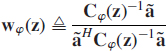
where ã = a(![]() ) is the nominal array response vector for fixed look direction
) is the nominal array response vector for fixed look direction ![]() (assumed to be known exactly).
(assumed to be known exactly).
Then the φ-MVDR beamformer-based DOA estimates can be found from the spectrum
![]()
If we are using weight φ ≡ 1 (in which case ![]() ), then the corresponding wφ(z) and Pφ(θ) correspond to the conventional MVDR beamformer weight functional
), then the corresponding wφ(z) and Pφ(θ) correspond to the conventional MVDR beamformer weight functional ![]() and spectrum PCAP(θ) in (2.29) and (2.31), respectively.
and spectrum PCAP(θ) in (2.29) and (2.31), respectively.
Define
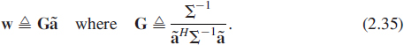
Since the M-functional Cφ(z) is proportional to Σ at FΣ, it follows that
![]()
provided that Cφ(FΣ) exists. Since in practice, the true Cφ is unknown, we replace it by the M-estimator ![]() , which yields
, which yields

as the plug-in estimator. The optimal weight at FΣ employs the MLE of Σ (i.e., φ = φml, where φml is given by (2.23)) and is hereafter denoted by ![]() .
.
![]() EXAMPLE 2.9
EXAMPLE 2.9
Our simulation setting is as follows. A k = 4 sensor ULA with λ/2 spacing received two (d = 2) uncorrelated circular Gaussian signals of equal variance ![]() with DOAs at −10° (SOI) and 15° (interferer). In the first setting (A), noise n has circular Gaussian distribution
with DOAs at −10° (SOI) and 15° (interferer). In the first setting (A), noise n has circular Gaussian distribution ![]() , and in the second setting (B), noise has circular Cauchy distribution
, and in the second setting (B), noise has circular Cauchy distribution ![]() . Note that the Cauchy distribution does not have finite variance and
. Note that the Cauchy distribution does not have finite variance and ![]() is the scale parameter of the distribution. In both A and B, the SNR (dB) is defined using scale parameters as
is the scale parameter of the distribution. In both A and B, the SNR (dB) is defined using scale parameters as ![]() . The number of snapshots is n = 500.
. The number of snapshots is n = 500.
Figure 2.8 depicts the estimated φ-MVDR beampatterns for look direction −10° for settings A and B averaged over 100 realizations. Also plotted are the estimated spectrums. The employed M-estimators are the SCM [i.e., HUB(1)], MLT(1) and HUB(0.9). In the Gaussian noise case (setting A), the beampatterns are similar, in fact, overlapping for SCM and HUB(0.9). The estimated spectrums associated with the different estimators are overlapping in the Gaussian case, so they provide essentially the same DOA estimates. In the Cauchy noise case (setting B), however, the conventional MVDR fails completely and can not resolve the two sources: the estimated beampattern and spectrum are flat and the mainlobe and the peaks cannot be well identified. Beampatterns associated with MLT(1) and HUB(0.9), however, show a narrow mainlobe centered at the look direction and a deep null at DOA of interference. Also spectrums for MLT(1) and HUB(0.9) show two sharp peaks at the DOAs of the sources. Hence the performance loss is negligible by employing MLT(1) or HUB(0.9) instead of the SCM in nominal Gaussian noise conditions. However, significant gain in performance is obtained when the noise is heavy-tailed Cauchy.
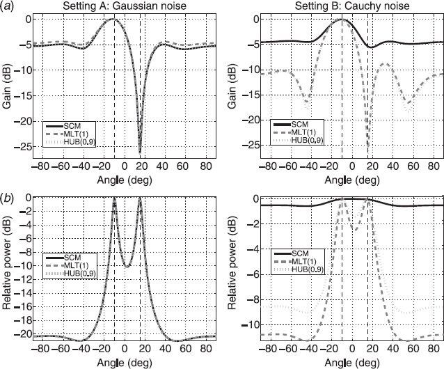
Figure 2.8 Averaged φ-MVDR beampatterns (a) and spectrums (b) for setting A and B (n = 500, SOI at −10°, interferer at 15°). In Gaussian noise, all estimators perform comparably. In Cauchy noise, SCM fails, but robust HUB(0.9) and MLT(1) estimators perform very well.
2.7.1 The Influence Function Study
First we derive the IF of the conventional MVDR functional. First note that the conventional MVDR functional can be written in the form
![]()
where
![]()
is the normalized steering vector that satisfies ![]() .
.
Applying the product rule of differentiation on the identity ![]() shows that
shows that
![]()
where ![]() is the value of the covariance matrix at the reference distribution F. Substituting the expression (2.17) for the IF of the covariance matrix
is the value of the covariance matrix at the reference distribution F. Substituting the expression (2.17) for the IF of the covariance matrix ![]() into the result above yields the following expression
into the result above yields the following expression
![]()
for the IF of the inverse of the covariance matrix.
Now, using the product rule of differentiation, the IF of the conventional MVDR functional ![]() can be split into two parts
can be split into two parts
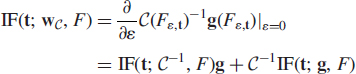
where g is the value of g(·) at F. The second part in the above IF expression can be written in the form

Thus, the IF of ![]() can now be written as
can now be written as
![]()
Using the IF expression (2.36) of the inverse of the covariance matrix shows that
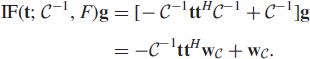
Thus the IF of ![]() can be written
can be written
![]()
By noting that ![]() (due to the MVDR gain constraint
(due to the MVDR gain constraint ![]() shows that
shows that
![]()
This is a compact expression for the IF of ![]() that also neatly reveals the vulnerability of the conventional MVDR weight vector to outliers. Clearly, contamination at a point t with large norm
that also neatly reveals the vulnerability of the conventional MVDR weight vector to outliers. Clearly, contamination at a point t with large norm ![]() has an effect proportional to
has an effect proportional to ![]() the IF. We may also rewrite the IF expression (2.37) as
the IF. We may also rewrite the IF expression (2.37) as
![]()
where ![]() and
and ![]() is a unit vector. This expression shows that the norm of the IF grows linearly with r (since u remains bounded).
is a unit vector. This expression shows that the norm of the IF grows linearly with r (since u remains bounded).
Let us now consider the case that the reference distribution F is a circular CES distribution FΣ = CEk(Σ, g). In this case, since ![]() and
and ![]() , the IF expression can be written as follows in Theorem 3.
, the IF expression can be written as follows in Theorem 3.
Theorem 3 The IF of the conventional MVDR functional ![]() at a circular CES distribution FΣ = CEk(Σ, g) is given by
at a circular CES distribution FΣ = CEk(Σ, g) is given by
![]()
where r2 = tHΣ−1t, u = Σ−1/2t/r a unit vector and w = Gã is defined in (2.35).
It is now interesting to compare the IF of wC(·) to the general expression of the IF of any φ-MVDR functional wφ(·) derived in [48] and stated below.
Theorem 4 With the notations as in Theorem 3, the influence function of φ-MVDR functional wφ(·) at a CES distribution FΣ = CEk(Σ, g) is given by
![]()
where σφ is the solution to (2.27) and

and δ is a positive real rva with the pdf (2.12).
Theorem 4 shows that the IF of wφ(·) is continuous and bounded if, and only if, φ(x)x is continuous and bounded. This follows by noting that when ![]() , or equivalently
, or equivalently ![]() , grow to infinity, u = Σ−1/2t/r remains bounded. Hence, to validate the qualitative robustness of φ-MVDR beamformers we only need to validate that φ(x)x is bounded. Theorem 4 also shows that IF(ã; wφ, FΣ) = 0, that is, if the contamination point t equals the array response ã, then it causes zero influence on the functional. We wish to point out that if wφ(·) is the conventional MVDR functional (i.e., φ ≡ 1), then the IF expression of Theorem 4 indeed gives the IF expression of Theorem 3. For example, wφ based on HUB(0.9) or MLT(1) functionals are robust, that is, they have continuous and bounded IFs, since their φ(·) functions are down-weighting observations with large magnitude as shown in Figures 2.4 and 2.5.
, grow to infinity, u = Σ−1/2t/r remains bounded. Hence, to validate the qualitative robustness of φ-MVDR beamformers we only need to validate that φ(x)x is bounded. Theorem 4 also shows that IF(ã; wφ, FΣ) = 0, that is, if the contamination point t equals the array response ã, then it causes zero influence on the functional. We wish to point out that if wφ(·) is the conventional MVDR functional (i.e., φ ≡ 1), then the IF expression of Theorem 4 indeed gives the IF expression of Theorem 3. For example, wφ based on HUB(0.9) or MLT(1) functionals are robust, that is, they have continuous and bounded IFs, since their φ(·) functions are down-weighting observations with large magnitude as shown in Figures 2.4 and 2.5.
We wish to point out that in beamforming literature, “robust” more commonly refers to robustness to steering errors (imprecise knowledge of the array response ã may be due to uncertainty in array element locations, steering directions and calibration errors) and robustness in the face of insufficient sample support that may lead to rank deficient SCM or inaccurate estimates of the array covariance matrix. Thus, the lack of robustness is caused by misspecified or uncertain system matrices or due to the fact that we do not have sufficient sample support to build up the rank of the array covariance and pseudocovariance matrices, not because of uncertainty in the probability models.
The diagonal loading of the SCM is one of the most popular techniques to overcome the problems in the modeling system matrix or rank deficiency. Then we use ![]() , in place of
, in place of ![]() , which may not be full rank and hence not invertible. For this type of robustness study, see for example, [12, 16, 23, 35] and references therein. Here the term “robust” refers to statistical robustness to outliers [26], commonly measured by the concept of the IF. We wish to point out that robustness (as measured by the IF) of the MVDR beamformer remains unaltered by diagonally loading the covariance matrx
, which may not be full rank and hence not invertible. For this type of robustness study, see for example, [12, 16, 23, 35] and references therein. Here the term “robust” refers to statistical robustness to outliers [26], commonly measured by the concept of the IF. We wish to point out that robustness (as measured by the IF) of the MVDR beamformer remains unaltered by diagonally loading the covariance matrx ![]() , that is, using
, that is, using ![]() , where γ is some constant diagonal loading term not dependent on the distribution F of z. Although (statistical) robustness of the MVDR weight functional is not improved with diagonal loading, it provides, however, other kinds of robustness by improving the condition number of the estimated array covariance matrix. Naturally, IF is an asymptotic concept, and it is not the correct tool to analyze the performance in sample starved scenarios.
, where γ is some constant diagonal loading term not dependent on the distribution F of z. Although (statistical) robustness of the MVDR weight functional is not improved with diagonal loading, it provides, however, other kinds of robustness by improving the condition number of the estimated array covariance matrix. Naturally, IF is an asymptotic concept, and it is not the correct tool to analyze the performance in sample starved scenarios.
![]() EXAMPLE 2.10
EXAMPLE 2.10
We now compute the EIFs of estimated φ-MVDR beamformer weights ![]() for data sets Zn = {z1, …, zn} simulated as in setting A of Example 2.9. In the setting A, the observed snapshots z1, …, zn form an i.i.d. random sample from four-variate circular complex normal distribution
for data sets Zn = {z1, …, zn} simulated as in setting A of Example 2.9. In the setting A, the observed snapshots z1, …, zn form an i.i.d. random sample from four-variate circular complex normal distribution ![]() with covariance matrix
with covariance matrix ![]() , where
, where ![]() denotes the array response matrix of ULA for DOAs at 10° (SOI) and 15° (interferer). Let the k = four-variate contaminating vector t be such that only the first component t1 = u1 + jυ1 is allowed to vary, and the remaining components have fixed values: ti = ãi, where ãi denotes the ith component of the array response ã. An informative picture on the effect of contamination t1 = u1 + jυ1 on
denotes the array response matrix of ULA for DOAs at 10° (SOI) and 15° (interferer). Let the k = four-variate contaminating vector t be such that only the first component t1 = u1 + jυ1 is allowed to vary, and the remaining components have fixed values: ti = ãi, where ãi denotes the ith component of the array response ã. An informative picture on the effect of contamination t1 = u1 + jυ1 on ![]() is obtained by the surface plot of the norm of the empirical influence function
is obtained by the surface plot of the norm of the empirical influence function ![]() with respect to υ1 and υ1. The EIFs in Figure 2.9 are averages over 100 realizations. Sample lengths are n = 50, 500, ∞, where the surface plots under n = ∞ correspond to the asymptotic value
with respect to υ1 and υ1. The EIFs in Figure 2.9 are averages over 100 realizations. Sample lengths are n = 50, 500, ∞, where the surface plots under n = ∞ correspond to the asymptotic value ![]() . As expected, we observe that when the sample size grows (from n = 50 to n = 500), the calculated EIF surfaces more accurately resemble the corresponding theoretical IF surface. However, at the small sample size (n = 50), the relative influence of an additional observation on the estimator is a bit larger than that the IF would indicate. The surface plots neatly demonstrate the nonrobustness of the conventional MVDR beamformer for both the finite and large sample cases: outlying points with large values of u1 and/or υ1 have bounded influence in the cases of HUB(0.9) or MLT(1) but large and unbounded influence when the conventional SCM is employed.
. As expected, we observe that when the sample size grows (from n = 50 to n = 500), the calculated EIF surfaces more accurately resemble the corresponding theoretical IF surface. However, at the small sample size (n = 50), the relative influence of an additional observation on the estimator is a bit larger than that the IF would indicate. The surface plots neatly demonstrate the nonrobustness of the conventional MVDR beamformer for both the finite and large sample cases: outlying points with large values of u1 and/or υ1 have bounded influence in the cases of HUB(0.9) or MLT(1) but large and unbounded influence when the conventional SCM is employed.

Figure 2.9 Averaged ![]() for the φ-MVDR beamformers that employ the SCM (a), HUB(0.9) estimator (b) and MLT(1) estimator (c). Sample Zn (n = 50, 500) are generated as in setting A of Example 2.9; n = ∞ corresponds to the plot of
for the φ-MVDR beamformers that employ the SCM (a), HUB(0.9) estimator (b) and MLT(1) estimator (c). Sample Zn (n = 50, 500) are generated as in setting A of Example 2.9; n = ∞ corresponds to the plot of ![]() . The contamination point
. The contamination point ![]() is such that t2 is fixed and only
is such that t2 is fixed and only ![]() is allowed to vary.
is allowed to vary.
Efficiency Study Using the IF of wφ(·) (cf. Theorem 4) and equations (2.19) and (2.20) as the definitions for the asymptotic covariance matrix and pseudo-covariance matrix of the estimator, the next theorem was proved in [48].
Theorem 5 With the notations as in Theorem 4, the asymptotic covariance matrix of the estimated φ-MVDR weight ![]() when sampling from FΣ = CEk(Σ, g) is
when sampling from FΣ = CEk(Σ, g) is
![]()
where

The asymptotic pseudo-covariance matrix of ![]() vanishes, that is, ASP(
vanishes, that is, ASP(![]() ; FΣ) = 0.
; FΣ) = 0.
Note that the ASC of ![]() depends on the selected M-estimator and on the functional form of the CES distribution FΣ only via the real-valued positive multiplicative constant λφ. (Observe that the matrix term G − wwH does not depend on the choice of φ and on FΣ only via Σ.) Hence comparisons of this single scalar index is needed only. It is a surprising result that ASP vanishes, which means that
depends on the selected M-estimator and on the functional form of the CES distribution FΣ only via the real-valued positive multiplicative constant λφ. (Observe that the matrix term G − wwH does not depend on the choice of φ and on FΣ only via Σ.) Hence comparisons of this single scalar index is needed only. It is a surprising result that ASP vanishes, which means that ![]() has asymptotic circular CN distribution.
has asymptotic circular CN distribution.
Note also that ASC(![]() ; FΣ) is singular and of rank k − 1 (since the nullspace of G − wwH has dimension 1 due to MVDR constraint wHã = 1, so (G − wwH)ã = 0). Thus the asymptotic CN distribution of
; FΣ) is singular and of rank k − 1 (since the nullspace of G − wwH has dimension 1 due to MVDR constraint wHã = 1, so (G − wwH)ã = 0). Thus the asymptotic CN distribution of ![]() is singular. This is an expected result since singular distributions commonly arise in constrained parameter estimation problems, where the constraint imposes a certain degree of deterministicity to the estimator.
is singular. This is an expected result since singular distributions commonly arise in constrained parameter estimation problems, where the constraint imposes a certain degree of deterministicity to the estimator.
Table 2.1 Asymptotic relative efficiencies of ![]() based on HUB(q) and MLT(ν) estimators at Φk, Tk, 5 and Tk, 1 distributions (and dimensions k = 2, 3, 5, 10). Recall that HUB(1) correspond to SCM
based on HUB(q) and MLT(ν) estimators at Φk, Tk, 5 and Tk, 1 distributions (and dimensions k = 2, 3, 5, 10). Recall that HUB(1) correspond to SCM
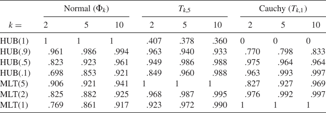
The asymptotic relative efficiency (ARE) of ![]() can thus be calculated as
can thus be calculated as
![]()
where λmle correspond to λφ value for the ![]() . Thus ARE (
. Thus ARE (![]() ; FΣ) ≤ 1. Table 2.1 reports the AREs of
; FΣ) ≤ 1. Table 2.1 reports the AREs of ![]() based on HUB(q) and MLT(ν) estimators under circular complex normal (Φk), circular complex Cauchy (Tk,1) and circular Tk,5 distributions for some choices of dimension k. Recall that the HUB(1) estimator corresponds to the SCM. At CN distribution, HUB(0.9) has the best performance among its robust alternatives. Furthermore, efficiencies for HUB(q) and MLT(ν) are increasing with the dimension: for example, at k = 10, HUB(0.9) experiences only 0.006 percent efficiency loss and MLT(1) which ranks the lowest, has a moderate 8.3 percent loss in efficiency. Hence adding more sensors to the array increases the (asymptotic) efficiency of the estimated φ-MVDR beamformers based upon the above robust M-estimators. At Tk,5 distribution, employed M-estimators are superior to the conventional MVDR beamformer based on SCM. At Cauchy distribution, all the robust M-estimators are performing very well and their efficiencies are increasing with the dimension. To conclude, these asymptotic efficiencies clearly favor φ-MVDR beamformers based upon robust M-estimators since they combine a high efficiency with appealing robustness properties.
based on HUB(q) and MLT(ν) estimators under circular complex normal (Φk), circular complex Cauchy (Tk,1) and circular Tk,5 distributions for some choices of dimension k. Recall that the HUB(1) estimator corresponds to the SCM. At CN distribution, HUB(0.9) has the best performance among its robust alternatives. Furthermore, efficiencies for HUB(q) and MLT(ν) are increasing with the dimension: for example, at k = 10, HUB(0.9) experiences only 0.006 percent efficiency loss and MLT(1) which ranks the lowest, has a moderate 8.3 percent loss in efficiency. Hence adding more sensors to the array increases the (asymptotic) efficiency of the estimated φ-MVDR beamformers based upon the above robust M-estimators. At Tk,5 distribution, employed M-estimators are superior to the conventional MVDR beamformer based on SCM. At Cauchy distribution, all the robust M-estimators are performing very well and their efficiencies are increasing with the dimension. To conclude, these asymptotic efficiencies clearly favor φ-MVDR beamformers based upon robust M-estimators since they combine a high efficiency with appealing robustness properties.
2.8 ROBUST ICA
Independent component analysis (ICA) is a relatively recent technique of multivariate data analysis and signal processing (see [14, 15, 28] and their bibliographies) used for example, in several applications including wireless communications, audio and speech signal separation, biomedical signal processing, image processing, feature extraction, and data-mining.
The main bulk of research in the field so far has concentrated on the real-valued ICA model, but the complex-valued ICA model has attained increasing interest during the last decade due to its potential applications, for example, for convolutive source separation in the frequency domain and for source separation of complex-valued data arising in several application areas such as magnetic resonance imaging (MRI) or antenna array signal processing (such as radar data). Therefore, many efforts have been pursued to establish identifiability/uniqueness/separability theory for complex-valued ICA model, to generalize existing techniques to complex case, and to derive new estimators that better exploit the specific nature of the complex-valued model; see [3, 5, 8, 11, 18, 19, 21, 22, 34, 39, 47, 49] to name only a few.
In this section, we assume that sensor outputs follow the noiseless complex-valued ICA model, that is
![]()
where ![]() has mutually statistically independent components s1, …, sd, and without any loss of generality, assume that E[s] = 0. As is common in ICA, we assume that the number of sources is equal to the number of sensors, so k = d and that the mixing matrix
has mutually statistically independent components s1, …, sd, and without any loss of generality, assume that E[s] = 0. As is common in ICA, we assume that the number of sources is equal to the number of sensors, so k = d and that the mixing matrix ![]() is nonsingular. Due to fundamental indeterminacy [22], ICA should be understood as the determination of a matrix
is nonsingular. Due to fundamental indeterminacy [22], ICA should be understood as the determination of a matrix ![]() , called the separating matrix, that satisfies
, called the separating matrix, that satisfies
![]()
where D is a k × k scaled permutation matrix, that is, ![]() contains permuted and scaled components of s. For the separation to be possible (up to above ambiguities), at most one of the sources can possess circular CN distribution, but sources can have CN distribution with distinct circularity coefficient [22].
contains permuted and scaled components of s. For the separation to be possible (up to above ambiguities), at most one of the sources can possess circular CN distribution, but sources can have CN distribution with distinct circularity coefficient [22].
We now review two classes of ICA estimators that are based on the concepts of (spatial) scatter and pseudo-scatter matrices.
2.8.1 The Class of DOGMA Estimators
Fourth Order Blind Identification (FOBI) method Assume for a moment that the source RV s has finite variances and therefore ![]() exists and is of full rank. Compute the whitening matrix
exists and is of full rank. Compute the whitening matrix ![]() as the square-root matrix of
as the square-root matrix of ![]() , that is,
, that is, ![]() . There exists many methods to compute B (e.g. Cholesky decomposition), but for our purposes, we do not need to specify any particular one. Then the whitened mixture v = Bz is uncorrelated, that is,
. There exists many methods to compute B (e.g. Cholesky decomposition), but for our purposes, we do not need to specify any particular one. Then the whitened mixture v = Bz is uncorrelated, that is, ![]() , and also follows the ICA model
, and also follows the ICA model
![]()
The identity ![]() shows that the scaled mixing matrix
shows that the scaled mixing matrix
![]()
is a unitary matrix, where σi = (E[|si|2])1/2. Since in any case, the scales of the columns ãi of à can not be identified due to fundamental indeterminacy of ICA, we may contend that à is a unitary matrix (without any loss of generality). Thus the separating matrix of the whitened mixture is a unitary matrix as well, so UHv = ![]() for some unitary matrix
for some unitary matrix ![]() , and thus W = UHB is a separating matrix for the original mixture. Cardoso [8] has shown that, if U = U(v) is the matrix of eigenvectors of kurtosis matrix
, and thus W = UHB is a separating matrix for the original mixture. Cardoso [8] has shown that, if U = U(v) is the matrix of eigenvectors of kurtosis matrix ![]() defined in (2.21), then the FOBI functional W(z) = U(v)HB(z) is a separating matrix provided that sources have finite and distinct circular kurtosis values, that is, κ0(si) ≠ κ0(sj) for all i ≠ j ∈ {1, …, k}, where κ0(·) is defined in (2.5).
defined in (2.21), then the FOBI functional W(z) = U(v)HB(z) is a separating matrix provided that sources have finite and distinct circular kurtosis values, that is, κ0(si) ≠ κ0(sj) for all i ≠ j ∈ {1, …, k}, where κ0(·) is defined in (2.5).
FOBI is perhaps the simplest method to solve the ICA problem proposed thus far. Since the FOBI functional can be computed via standard matrix decompositions operating on matrices ![]() and
and ![]() , it is also computationally (among) the most efficient approaches to ICA. It has some drawbacks, however. First, the necessity of distinct circular kurtosis values restricts the applicability of the method to some extent since sources with identical distributions (and hence with identical kurtosis) may occur frequently in some applications. Second, the assumption on finite kurtosis clearly confines permissible distributions of the sources the method can separate since fourth-order moments do not exist for many heavy-tailed distributions. Third, the method is not robust, since the covariance matrix (used for whitening) and the kurtosis matrix are highly non-robust.
, it is also computationally (among) the most efficient approaches to ICA. It has some drawbacks, however. First, the necessity of distinct circular kurtosis values restricts the applicability of the method to some extent since sources with identical distributions (and hence with identical kurtosis) may occur frequently in some applications. Second, the assumption on finite kurtosis clearly confines permissible distributions of the sources the method can separate since fourth-order moments do not exist for many heavy-tailed distributions. Third, the method is not robust, since the covariance matrix (used for whitening) and the kurtosis matrix are highly non-robust.
In order to separate sources with identical distribution and identical kurtosis, FOBI was later generalized to joint approximate diagonalization of eigen-matrices (JADE) [9, 11] which is based on joint diagonalization of several cumulant matrices. However, JADE still demands finite fourth-order moments, is not robust, and has the disadvantage that simplicity and computational efficiency of the FOBI algorithm is lost.
Generalization of FOBI Let C1(·) denote any scatter matrix and C2(·) denote any spatial scatter matrix functional with IC-property, by which we mean that if s has independent components, then C1(s) and C2(s) are diagonal matrices, that is
![]()
One can easily verify that the covariance matrix ![]() and the kurtosis matrix
and the kurtosis matrix ![]() possess IC-property. M-functionals of scatter Cφ(·) do not in general satisfy IC-property. However, if the sources si are assumed to be symmetric, that is, si =d −si for i = 1, …, k, then the requirement of IC-property can be dropped [47], since for symmetric independent sources, any scatter or spatial scatter matrix automatically possess the IC-property. Even if the sources are not symmetric, a symmetricized version of M-estimator (or of any scatter or spatial scatter matrix) can be easily constructed that automatically possesses IC-property, see [47, 49] for details.
possess IC-property. M-functionals of scatter Cφ(·) do not in general satisfy IC-property. However, if the sources si are assumed to be symmetric, that is, si =d −si for i = 1, …, k, then the requirement of IC-property can be dropped [47], since for symmetric independent sources, any scatter or spatial scatter matrix automatically possess the IC-property. Even if the sources are not symmetric, a symmetricized version of M-estimator (or of any scatter or spatial scatter matrix) can be easily constructed that automatically possesses IC-property, see [47, 49] for details.
DOGMA (Diagonalization Of Generalized covariance MAtrices) algorithm: DOGMA functional W(z) ∈ Ck×k is calculated as follows.
(a) Calculate the square-root matrix B1(z) of C1(z)−1, so B1(z)HB1(z) = C1(z)−1, and the whitened data v = B1(z)z (so C1(v) = I).
(b) Calculate the EVD of C2(F) of the whitened data
![]()
where Λ2(v) is a diagonal matrix of eigenvalues of C2(v) and U2(v) is a unitary matrix with the respective eigenvectors as columns.
(c) Set W(z) = U2(v)HB1(z).
Note that FOBI is a DOGMA functional W(z) with choices C1 = ![]() and
and ![]() Since the IC-property is required, the spatial sign covariance matrix
Since the IC-property is required, the spatial sign covariance matrix ![]() sgn (F) for example can not be employed as the choice of C2 unless sources have symmetric distributions. We wish to point out that W(z) = U2 (v)H B1 (z) simultaneously diagonalizes C1(z) and C2(z), namely, for transformed data
sgn (F) for example can not be employed as the choice of C2 unless sources have symmetric distributions. We wish to point out that W(z) = U2 (v)H B1 (z) simultaneously diagonalizes C1(z) and C2(z), namely, for transformed data ![]() = W(z)z it holds that
= W(z)z it holds that
![]()
Hence, we call the above algorithm DOGMA (Diagonalization Of Generalized covariance MAtrices).
Note that in the step (b) of the algorithm Λ2 (v) = diag(δ1, …, δk) is a diagonal matrix with eigenvalues δ1, …, δk of C2 (v) on its diagonal elements. It can be shown (cf. Theorem 1 of [49]) that
![]()
For example, in the case of the FOBI functional (i.e., C1 = C and C2 = Ckur), the eigenvalues are easily calculated as

where κ0,i = κ0 (si) denotes the circular kurtosis of the ith source rva si.
The following result has been proved in [49].
Theorem 6 Under the assumptions
D1: C1(s) and C2(s) exists, and
D2: eigenvalues δ1, …, δk of C2(v) are distinct, that is, δi ≠ δj for all i ≠ j ∈ {1, …, k}, the DOGMA functional W(z) = U2(v)HB1(z) is a separating matrix for the complex-valued ICA model.
As an example, consider the FOBI functional. Then, the assumption D1 is equivalent with the assumption that sources has finite circular kurtosis values. Assumption D2 implies (due to (2.41)) that sources have distinct values of circular kurtosis, that is, κ0 (si) ≠ κ0 (sj) for all i ≠ j ∈ (1, …, k).
For more properties of DOGMA functionals, see [49], where also alternative formulations of the method are derived along with efficient computational approach to compute the estimator.
2.8.2 The Class of GUT Estimators
Let C(·) denote any scatter matrix functional and P(·) denote any spatial pseudo-scatter matrix functional with IC-property (i.e., they reduce to diagonal matrices when F is a cdf of a random vector with independent components). As already mentioned, the covariance matrix is an example of a scatter matrix that possesses IC-property. Pseudo-kurtosis matrix ![]() kur (·) defined in (2.21) is an example of a spatial pseudo-scatter matrix that possesses IC-property. Sign pseudo-covariance matrix
kur (·) defined in (2.21) is an example of a spatial pseudo-scatter matrix that possesses IC-property. Sign pseudo-covariance matrix ![]() sgn (·) for example do not necessarily possess IC-property. However, as mentioned earlier, for symmetric independent sources, any scatter or spatial pseudo-scatter matrix automatically possesses IC-property. Again if the sources are not symmetric, a symmetricized version of any scatter or spatial pseudo-scatter matrix can be easily constructed that automatically possesses IC-property, see [47, 49] for details.
sgn (·) for example do not necessarily possess IC-property. However, as mentioned earlier, for symmetric independent sources, any scatter or spatial pseudo-scatter matrix automatically possesses IC-property. Again if the sources are not symmetric, a symmetricized version of any scatter or spatial pseudo-scatter matrix can be easily constructed that automatically possesses IC-property, see [47, 49] for details.
Definition 5 Matrix functional ![]() of
of ![]() is called the Generalized Uncorrelating Transform (GUT) if transformed data s = Wz satisfies
is called the Generalized Uncorrelating Transform (GUT) if transformed data s = Wz satisfies
![]()
where Λ = Λ(s) = diag(λi) is a real nonnegative diagonal matrix, called the circularity matrix, and ![]() is called the ith circularity coefficient, i = 1, …, k.
is called the ith circularity coefficient, i = 1, …, k.
The GUT matrix with choices C = ![]() and P =
and P = ![]() corresponds to the SUT [21, 22] described in Section 2.2.2. Essentially, GUT matrix W(·) is a data transformation that jointly diagonalizes the selected scatter and spatial pseudo-scatter matrix of the transformed data s = Wz. Note that the pseudo-covariance matrix employed by SUT is a pseudo-scatter matrix, whereas in Definition 5, we only require C(·) to be a spatial pseudo-scatter matrix.
corresponds to the SUT [21, 22] described in Section 2.2.2. Essentially, GUT matrix W(·) is a data transformation that jointly diagonalizes the selected scatter and spatial pseudo-scatter matrix of the transformed data s = Wz. Note that the pseudo-covariance matrix employed by SUT is a pseudo-scatter matrix, whereas in Definition 5, we only require C(·) to be a spatial pseudo-scatter matrix.
GUT algorithm
(a) Calculate the square-root matrix B(z) of C(z)−1, so B(z)H B(z) = C(z)−1, and the whitened data v = B(z)z (so C(v) = I).
(b) Calculate Takagi's factorization (symmetric SVD) of P(·) for the whitened data v
![]()
where ![]() is a unitary matrix (i.e., the Takagi factor of P(v)) and Λ is the circularity matrix (i.e., the singular values of P(v) are the circularity coefficients λi = [P(s)]ii appearing in (2.42)).
is a unitary matrix (i.e., the Takagi factor of P(v)) and Λ is the circularity matrix (i.e., the singular values of P(v) are the circularity coefficients λi = [P(s)]ii appearing in (2.42)).
(c) Set W(z) = U(v)H B(z).
In step (a), the data is whitened in the sense that C(v) = I. Naturally, if the selected scatter matrix is the covariance matrix, then the data is whitened in the conventional sense. Since the whitening transform B is unique only up to left-multiplication by a unitary matrix, GUT matrix W = UH B is also a whitening transform in the conventional sense but with an additional property that it diagonalizes the selected spatial pseudo-scatter matrix.
As revealed in step (b) of the algorithm, the circularity matrix Λ = diag(λi) has singular values λ1, …, λk of P(v) as its diagonal elements. It has been shown in Theorem 3 of [47] that the circularity coefficient is
![]()
where ![]() denotes the whitened source whose ith component is
denotes the whitened source whose ith component is ![]() For example, consider the SUT functional (i.e., C =
For example, consider the SUT functional (i.e., C = ![]() , P =
, P = ![]() ). Then
). Then
![]()
that is, the ith circularity coefficient is equal to the circularity coefficient of the ith source si. Next consider the case that the GUT functional employs C = ![]() and P =
and P = ![]() kur. Then
kur. Then
![]()
Hence the ith circularity coefficient λi is the modulus of a weighted sum of a 4th-order and 2nd-order moment of the ith whitened source ![]() .
.
The following result has been proved in [47].
Theorem 7 Under the assumptions
G1: C(s) and P(s) exists, and
G2: circularity coefficients λ1, …, λk (the singular values of P(v) are distinct, that is, λi ≠ λj for all i ≠ j ∈ {1, …, k}, the GUT functional W(z) = U(v)HB(z) is a separating matrix for the complex-valued ICA model.
As an example, consider the SUT functional. Then assumption G1 is equivalent with the assumption that sources has finite variances. Assumption G2 implies (due to (2.44)) that sources have distinct circularity coefficients.
It is important to observe that the GUT algorithm contains a built-in warning: since the circularity coefficients λ1, …, λk are also necessarily extracted, then the detection of two close or almost equal circularity coefficients is an indication that the corresponding sources may not be reliably separated. Also, assumption G2 is needed to separate all the sources: GUT matrix is not able to separate the sources that have identical circularity coefficients, but the rest of the sources are separated; cf. [47].
For more properties of GUT functionals, see [47], where also alternative formulations of the method are derived along with efficient computational approaches to compute the estimator.
2.8.3 Communications Example
Let ![]() denote an estimator of the separating matrix. The performance of the separation is often investigated via interference matrix
denote an estimator of the separating matrix. The performance of the separation is often investigated via interference matrix ![]() . Due to fundamental indeterminacy of ICA, perfect separation implies that
. Due to fundamental indeterminacy of ICA, perfect separation implies that ![]() is a scaled permutation matrix. The quality of the separation is then assessed by calculating the widely used performance index (PI) [2]
is a scaled permutation matrix. The quality of the separation is then assessed by calculating the widely used performance index (PI) [2]

where ![]() . Under perfect separation
. Under perfect separation ![]() When the estimator fails to separate the sources, the value of the PI increases. The PI is scaled so that the maximum value is 1. If the separating matrix estimator
When the estimator fails to separate the sources, the value of the PI increases. The PI is scaled so that the maximum value is 1. If the separating matrix estimator ![]() is equivariant (in the sense advocated in [10], Section II-C), as is the case for GUT and DOGMA estimators, then
is equivariant (in the sense advocated in [10], Section II-C), as is the case for GUT and DOGMA estimators, then ![]() (and thus PI) does not depend on the mixing matrix A, and hence one could set A = I in the simulations without any loss of generality.
(and thus PI) does not depend on the mixing matrix A, and hence one could set A = I in the simulations without any loss of generality.
In our simulation studies, GUT estimators employing the following choices of scatter matrix C and spatial pseudo-scatter matrix P are used: gut1 employs covariance matrix and pseudo-covariance matrix (i.e., SUT), gut2 employs covariance matrix and pseudo-kurtosis matrix, gut3 employs covariance matrix and sign pseudo-covariance matrix (SPM), gut4 employs HUB (0.9) estimator and SPM, gut5 employs Tyler's M-estimator of scatter and SPM. We compare the results to jade [11], fobi [8], complex FastICA with deflationary approach and contrast G2(x) = log (0.1 + x) [5] (denoted as fica), complex fixed point algorithm using kurtosis based contrast and symmetric orthogonalization [19] (denoted as cfpa), gradient based kurtosis maximization algorithm [34] (denoted as kmg) and DOGMA estimator employing Tyler's M-estimator and HUB (0.9) estimator as the choices of scatter matrices C1 (·) and C2 (·), respectively (denoted as d1).
In our simulation setting, three independent random signals—a BPSK signal, a 8-QAM signal and a circular Gaussian signal of equal power ![]() are impinging on k = 3 element Uniform Linear Array (ULA) with half a wavelength interelement spacing from DOAs −20°, 5° and 35°. Note that BPSK and 8-QAM signals are second-order non-circular. The above random communications signals are symmetric, and hence any pair of scatter and spatial pseudo-scatter matrices can be employed in the definition of the GUT matrix and DOGMA matrix. The array outputs are corrupted by additive noise n with a circular complex Gaussian distribution with covariance matrix
are impinging on k = 3 element Uniform Linear Array (ULA) with half a wavelength interelement spacing from DOAs −20°, 5° and 35°. Note that BPSK and 8-QAM signals are second-order non-circular. The above random communications signals are symmetric, and hence any pair of scatter and spatial pseudo-scatter matrices can be employed in the definition of the GUT matrix and DOGMA matrix. The array outputs are corrupted by additive noise n with a circular complex Gaussian distribution with covariance matrix ![]() . The signal to noise ratio (SNR) is
. The signal to noise ratio (SNR) is ![]() and the number of snapshots is n = 2000. The estimated source signal constellations obtained by jade and gut5 are shown in Figure 2.10. Both of the methods were able to separate the sources as BPSK, 8-QAM and circular Gaussian source signals are clearly discernible. Table 2.2. shows the average performance of all the ICA estimators over 100 simulation runs. jade and kmg are performing the best but GUT methods are not far behind. fobi and d1, however, stand out as they do not quite reach the same level of performance as the others.
and the number of snapshots is n = 2000. The estimated source signal constellations obtained by jade and gut5 are shown in Figure 2.10. Both of the methods were able to separate the sources as BPSK, 8-QAM and circular Gaussian source signals are clearly discernible. Table 2.2. shows the average performance of all the ICA estimators over 100 simulation runs. jade and kmg are performing the best but GUT methods are not far behind. fobi and d1, however, stand out as they do not quite reach the same level of performance as the others.

Figure 2.10 Estimated source signal constellations obtained by jade (a) and GUT method gut5 (b). BPSK, 8-QAM and circular Gaussian source signals are clearly discernible on the left, middle and right plots.
Table 2.2 Mean values of − 10 log10 [PI(![]() )] computed from 100 array snapshot data sets
)] computed from 100 array snapshot data sets
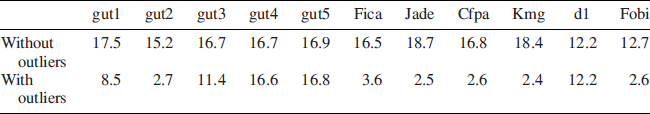

Figure 2.11 Estimated source signal constellations obtained by jade (a) and GUT method gut5 (b) for the data with four outliers. Signals that correspond to outliers are marked by triangle. Robust GUT method gut5 is unaffected by outliers, which are clearly detected in the plots whereas jade fails completely: outliers are able to destroy the patterns of BPSK and 8-QAM signals.
To illustrate the reliable performance of the robut GUT matrices under contamination, four observations were replaced by an outlier zout generated as
![]()
where zi,max is the element of the ith row of the sample data matrix ![]() with largest modulus, ui ~ Unif(1,5) and bi is a rva with a value of −1 or 1 with equal probability
with largest modulus, ui ~ Unif(1,5) and bi is a rva with a value of −1 or 1 with equal probability ![]() . Note that zi, out = bi ui zi,max points to the same or opposite direction as zi,max but its magnitude is at least as big, but at most 5 times larger than that of zi,max. Note that only 0.2 percent (4 observations out of n = 2000) of the data is contaminated. Figure 2.11 depicts the estimated source signal constellations obtained by jade and gut5. As can be seen, only gut5 is able to separate the sources and is unaffected by outliers, which are clearly detected in the plots. jade on the other hand fails completely: BPSK and 8-QAM sources are no longer discernible in the plots. The reliable performance of the robust ICA methods is evident in Table 2.2.: only the robust GUT methods gut4 and gut5 and the robust DOGMA estimator d1 are able to separate the sources.
. Note that zi, out = bi ui zi,max points to the same or opposite direction as zi,max but its magnitude is at least as big, but at most 5 times larger than that of zi,max. Note that only 0.2 percent (4 observations out of n = 2000) of the data is contaminated. Figure 2.11 depicts the estimated source signal constellations obtained by jade and gut5. As can be seen, only gut5 is able to separate the sources and is unaffected by outliers, which are clearly detected in the plots. jade on the other hand fails completely: BPSK and 8-QAM sources are no longer discernible in the plots. The reliable performance of the robust ICA methods is evident in Table 2.2.: only the robust GUT methods gut4 and gut5 and the robust DOGMA estimator d1 are able to separate the sources.
Table 2.3 gives average computation times. As can be seen gut1 (i.e., the SUT) and fobi are the fastest to compute whereas fica is the slowest. To compute fobi we used the fast algorithm of [49]. Also observe that the occurrence of outliers severely increases the computation times of the iterative fixed-point algorithms fica, kmg and cfpa, whereas computation times for the other methods are only slightly affected by outliers.
Table 2.3 Average computation times (in milliseconds) over 100 runs for array snapshot data sets without outliers and with four outliers generated as zout

2.9 CONCLUSION
In this chapter we focused on multichannel signal processing of complex-valued signals in cases where the underlying ideal assumptions on signal and noise models do not necessarily hold. We considered departures from two key assumptions, that is circularity of the signal and/or noise as well as Gaussianity of the noise distribution. A comprehensive description of the full second-order statistics of complex random vectors was provided since the conventional covariance matrix alone suffices only in the case of circular signals. A detection scheme for noncircularity was developed. This facilitates using the full second-order statistics of the signals and appropriate algorithms in the presence of noncircularity. Moreover, estimators and multichannel signal processing algorithms that also take into account the noncircularity of the signals and are robust in the face of heavy-tailed noise were introduced. Their robustness and efficiency were analyzed. Example applications in beamforming, subspace-based direction finding and blind signal separation were presented.
2.10 PROBLEMS
2.1 Show that circularity coefficient λ(z) satisfies (2.3) and (2.4).
2.2 Based on the definition qn of the GLRT decision statistic, derive the equation (2.13) for ln and verify using arguments based on the properties of eigenvalues that the test statistic ln is invariant under invertible linear transformations of the data.
2.3 MATLAB assignment. Let us have a uniform linear array of eight elements. Two QPSK modulated signals are impinging on the array from directions of arrival 72° and 66°. Our N = 200 observations are contaminated by complex white second order circular Gaussian noise such that the signal to noise ratio (SNR) is 10 dB. Plot the MUSIC pseudo-spectrum. Study the traces of array covariance and pseudo-covariance matrices. What can you say about the circularity of the observations?
2.4 MATLAB assignment. Let us have similar array configuration as above. Now two BPSK modulated signals are impinging the array. Our N = 200 observations are contaminated by complex white second order circular Gaussian noise such that the signal to noise ratio (SNR) is 10 dB. Plot the MUSIC pseudo spectrum. Study the traces of array covariance and pseudo-covariance matrices. What can you say about the circularity of the observations?
2.5 MATLAB assignment. Consider again a uniform linear array of eight elements. Two QPSK modulated signals are impinging on the array from directions of arrival 72° and 66°. Now we have an ε-contaminated noise model obeying mixture of two complex second order circular Gaussian distributions f(n) = (1 − ε) f (0, σ2 I) + ε f (0, 50σ2 I). With ε = 0.1 we have 10 percent outliers present in the sample. The signal to noise ratio would be 10 dB in the absence of outliers. Plot the MUSIC pseudo-spectrum using sample covariance matrix based estimator and sign covariance matrix based estimator. What can you say about the robustness of the estimators?
2.6 MATLAB assignment. Write a function called glrtcirc(Z) for the GLRT test statistic −n ln ln of circularity, where the argument Z of the function is a k × n snapshot data matrix. After doing so,
a) generate k × n data matrix Z consisting of n indenpendent random samples from circular Tk,υ using result (2.14). Transform the data by Z → S = GZ, where G can be any nonsingular k × k matrix. Then verify that computed values of test statistics glrtcirc(Z) and glrtcirc(S) coincide, meaning that GLRT test statistic is invariant under invertible linear data transformations.
b) Write a function for the adjusted GLRT test statistic ![]() of circularity and reproduce the chi-square plots of Figure 2.2.
of circularity and reproduce the chi-square plots of Figure 2.2.
2.7 Show that the kurtosis matrix ![]() kur (·) and the pseudo-kurtosis matrix
kur (·) and the pseudo-kurtosis matrix ![]() kur (·) defined in (2.21) possess IC-property. If sources are symmetric, that is, si = d − si, for i = 1, …, d, then show that any scatter matrix C (·) or pseudo-scatter matrix P(·) possess IC-property.
kur (·) defined in (2.21) possess IC-property. If sources are symmetric, that is, si = d − si, for i = 1, …, d, then show that any scatter matrix C (·) or pseudo-scatter matrix P(·) possess IC-property.
REFERENCES
1. H. Abeida and J.-P. Delmas, MUSIC-like estimation of direction of arrival for noncircular sources. IEEE Trans. Signal Processing, 54(7), (2006).
2. S. I. Amari, A. Cichocki, and H. H. Yang, “A new learning algorithm for blind source separation,” in D. S. Touretzky, M. C. Mozer, and M. E. Hasselmo, Eds., Advances in Neural Information Processing Systems 8, pages 757–763. MIT Press, Cambridge, MA, (1996).
3. J. Anemüller, T. J. Sejnowski, and S. Makeig, Complex independent component analysis of frequency-domain electroencephalographic data. Neural Networks, 16: 1311–1323, (2003).
4. P. Billingsley, Probability and Measure (3rd ed). Wiley, New York, 1995.
5. E. Bingham and A. Hyvarinen, A fast fixed-point algorithm for independent component analysis of complex-valued signals. Int. J. of Neural Systems, 10(1): 1–8, (2000).
6. D. H. Brandwood, A complex gradient operator and its applications in adaptive array theory. IEE Proc. F and H, 1: 11–16, (1983).
7. J. Capon, High resolution frequency-wavenumber spectral analysis. Proceedings of the IEEE, 57(8): 1408–1418, (1969).
8. J. F. Cardoso, “Source separation using higher order moments,” in Proc. IEEE Int. Conf. on Acoustics, Speech and Signal Processing (ICASSP'89), pages 2109–2112, Glasgow, UK, 1989.
9. J. F. Cardoso, High-order contrasts for independent component analysis. Neural Computation, 11(1): 157–192, (1999).
10. J.-F. Cardoso and B. H. Laheld, Equivariant adaptive source separation. IEEE Trans. Signal Processing, 44(12): 3017–3030, (1996).
11. J. F, Cardoso and A. Souloumiac, Blind beamforming for non-gaussian signals. IEE Proceedings-F, 140(6): 362–370, (1993).
12. B. D. Carlson, Covariance matrix estimation errors and diagonal loading in adaptive arrays. IEEE Trans. Aerosp. Electron. Syst., 24(4): 397–401, (1988).
13. P. Chargé, Y. Wang, and J. Saillard, A non-circular sources direction finding methods using polynomial rooting. Signal Processing, 81: 1765–1770, (2001).
14. A. Cichocki and S-I. Amari, Adaptive Blind Signal and Image Processing. John Wiley, New York, 2002.
15. P. Comon, Independent component analysis—a new concept? Signal Processing, 36: 287–314, (1994).
16. H. Cox, R. M. Zeskind, and M. M. Owen, Robust adaptive beamforming. IEEE Trans. Acoust., Speech, Signal Processing, 35(10): 1365–1376, (1987).
17. C. Croux, Limit behavior of the empirical influence function of the median. Statistics & Probability Letters, 37: 331–340, (1998).
18. L. De Lathauwer and B. De Moore, “On the blind separtion of non-circular source,” in Proc. 11th European Signal Processing Conference (EUSIPCO 2002), Toulouse, France, September 2002.
19. S. C. Douglas, Fixed-point algorithms for the blind separation of arbitrary complex-valued non-gaussian signal mixtures. EURASIP J. Advances in Signal Processing, 2007 (Article ID 36525, 15 pages), (2007).
20. Scott C. Douglas, “Fixed-point FastICA algorithms for the blind separation of complex-valued signal mixtures,” in Proc. 39th Asilomar Conf. on Signals, Systems and Computers (ACSSC'05), pages 1320–1325, 2005.
21. J. Eriksson and V. Koivunen, “Complex-valued ICA using second order statistics,” in Proc. IEEE Workshop on Machine Learning for Signal Processing (MLSP'04), Sao Luis, Brazil, 2004.
22. J. Eriksson and V. Koivunen, Complex random vectors and ICA models: Identifiability, uniqueness and seperability. IEEE Trans. Inform. Theory, 52(3): 1017–1029, (2006).
23. A. B. Gershman, “Robust adaptive beamforming: an overview of recent trends and advances in the field,” in Proc. 4th International Conference on Antenna Theory and Techniques, pages 30–35, September 9–12, 2003.
24. N. R. Goodman, Statistical analysis based on certain multivariate complex Gaussian distribution (an introduction). Annals Math. Statist., 34: 152–177, (1963).
25. M. Haardt and F. Römer, “Enhancements of unitary ESPRIT for non-circular sources,” in Proc. Int. Conf. Acoustics, Speech and Signal Processing (ICASSP'04), Montreal, Canada, May 2004.
26. F. R. Hampel, E. M. Ronchetti, P. J. Rousseeuw, and W. A. Stahel, Robust Statistics: The Approach Based on Influence Functions. Wiley, New York, 1986.
27. P. J. Huber, Robust Statistics. Wiley, New York, 1981.
28. A. Hyvärinen, J. Karhunen, and E. Oja, Independent Component Analysis. John Wiley, New York, 2001.
29. S. M. Kay, Fundamentals of Statistical Signal Processing. Prentice-Hall, New Jersey, 1993.
30. J. T. Kent, Data analysis for shapes and images. J. Statist. Plann. Inference, 57: 181–193, (1997).
31. J. T. Kent and D. E. Tyler, Redescending M-estimates of multivariate location and scatter. Ann. Statist., 19(4): 2102–2119, (1991).
32. H. Krim and M. Viberg, Two decades of array signal processing: the parametric approach. IEEE Signal Processing Mag., 13(4): 67–94, (1996).
33. P. R. Krishnaiah and J. Lin, Complex elliptically symmetric distributions. Comm. Statist. - Th. and Meth., 15: 3693–3718, (1986).
34. H. Li and T. Adalı, A class of complex ICA algorithms based on the kurtosis cost function. IEEE Trans. Neural Networks, 19(3): 408–420, (2008).
35. J. Li, P. Stoica, and Z. Wang, On robust capon beamforming and diagonal loading. IEEE Trans. Signal Processing, 51(7): 1702–1715, (2003).
36. G. M. Manolakis, K. I. Vinay, and S. M. Kogon, Statistical and adaptive signal processing. McGraw-Hill, Singapore, 2000.
37. R. A. Maronna, Robust M-estimators of multivariate location and scatter. Ann. Statist., 5(1): 51–67, (1976).
38. F. D. Neeser and J. L. Massey, Proper complex random processes with applications to information theory. IEEE Trans. Inform. Theory, 39(4): 1293–1302, (1993).
39. M. Novey and T. Adalı, On extending the complex FastICA algorithm to noncircular sources. IEEE Trans. Signal Processing, 56(5), (2008).
40. E. Ollila and V. Koivunen, “Adjusting the generalized likelihood ratio test of circularity robust to non-normality,” in Proc. 10th IEEE Int. Workshop on Signal Processing Advances in Wireless Comm. (SPAWC'09), pages 558–562, Perugia, Italy, June 21–24, 2009.
41. E. Ollila, On the circularity of a complex random variable. IEEE Signal Processing Letters, 15: 841–844, (2008).
42. E. Ollila, J. Eriksson, and V. Koivunen, Complex univariate distributions – part II: complex normal distribution and its extensions. Technical report, Signal Processing Labaratory, Helsinki Univerisity of Technology, 02150 Espoo, Finland, 2006.
43. E. Ollila and V. Koivunen, “Influence functions for array covariance matrix estimators,” in Proc. IEEE Workshop on Statistical Signal Processing (SSP'03), pages 445–448, St. Louis, USA, September 28– Oct. 1, 2003.
44. E. Ollila and V. Koivunen, “Robust antenna array processing using M-estimators of pseudo-covariance,” in Proc. 14th IEEE Int. Symp. on Personal, Indoor and Mobile Radio Comm. (PIMRC'03), pages 2659–2663, Beijing, China, September 7–10, 2003.
45. E. Ollila and V. Koivunen, “Robust space-time scatter matrix estimator for broadband antenna arrays,” in Proc. 58th IEEE Vehicular Technology Conference (VTC'03-Fall), volume 1, pages 55–59, Orlando, USA, October 6–9, 2003.
46. E. Ollila and V. Koivunen, “Generalized complex elliptical distributions,” in Proc. Third IEEE Sensor Array and Multichannel Signal Processing Workshop (SAM'04), Barcelona, Spain, June 18–21, 2004.
47. E. Ollila and V. Koivunen, Complex ICA using generalized uncorrelating transformation. Signal Processing, 89(4): 365–377, (2009).
48. E. Ollila and V. Koivunen, Influence function and asymptotic efficiency of scatter matrix based array processors: case MVDR beamformer. IEEE Trans. Signal Processing, 57(1): 247–259, (2009).
49. E. Ollila, H. Oja, and V. Koivunen, (in press) Complex-valued ICA based on a pair of generalized covariance matrices. Computational Statistics and Data Analysis, 52(7): 3789–3805, (2008).
50. B. Picinbono, On circularity. IEEE Trans. Signal Processing, 42(12): 3473–3482, (1994).
51. B. Picinbono, Second order complex random vectors and normal distributions. IEEE Trans. Signal Processing, 44(10): 2637–2640, (1996).
52. B. Picinbono and P. Chevalier, Widely linear estimation with complex data. IEEE Trans. Signal Processing, 43(8): 2030–2033, (1995).
53. P. J. Schreier and L. L. Scharf, Second-order analysis of improper complex random vectors and processes. IEEE Trans. Signal Processing, 51(3): 714–725, (2003).
54. P. J. Schreier, L. L. Scharf, and A. Hanssen, A generalized likelihood ratio test for impropriety of complex signals. IEEE Signal Processing Letters, 13(7): 433–436, (2006).
55. P. Stoica and R. Moses, Introduction to spectral analysis. Prentice-Hall, Upper Saddle River, 1997.
56. P. Tsakalides and C. L. Nikias, The robust covariation based MUSIC (roc-MUSIC) algorithm for bearing estimation in impulsive noise environments. IEEE Trans. Signal Processing, 44(7): 1623–1633, (1995).
57. A. van den Bos, The multivariate complex normal distribution–a generalization. IEEE Trans. Inform. Theory, 41(2): 537–539, (1995).
58. B. D. Van Veen and K. M. Buckley, Beamforming: a versatile approach to spatial filtering. IEEE ASSP magazine, April (1988).
59. S. Visuri, H. Oja, and V. Koivunen, Subspace-based direction of arrival estimation using nonparametric statistics. IEEE Trans. Signal Processing, 49(9): 2060–2073, (2001).
60. T. Wax and T. Kailath, Detection of signals by information theoretic criteria. IEEE Trans. Acoust., Speech, Signal Processing, 33(2): 387–392, (1985).
61. R. A. Wooding, The multivariate distribution of complex normal variables. Biometrika, 43: 212–215, (1956).
Adaptive Signal Processing: Next Generation Solutions. Edited by Tülay Adalı and Simon Haykin
Copyright © 2010 John Wiley & Sons, Inc.