6

NONLINEAR SEQUENTIAL STATE ESTIMATION FOR SOLVING PATTERN-CLASSIFICATION PROBLEMS

Simon Haykin and Ienkaran Arasaratnam

McMaster University, Canada

6.1 INTRODUCTION

Sequential state estimation has established itself as one of the essential elements of signal processing and control theory. Typically, we think of its use being confined to dynamic systems, where we are given a set of observables and the requirement is to estimate the hidden state of the system on which the observables are dependant. However, when the issue of interest is that of pattern-classification (recognition), we usually do not think of sequential estimation as a relevant tool for solving such problems. Perhaps, this oversight may be attributed to the fact that pattern-classification machines are usually viewed as static rather than dynamic systems. In this chapter, we take a different view: Specifically, we look to nonlinear sequential state estimation as a tool for solving pattern-classification problems, where the problem is solved through an iterative supervised learning process. In so doing, we demonstrate that this approach to solving pattern-classification problems offers several computational advantages compared to traditional methods, particularly when the problem of interest is difficult or large-scale.

The chapter is structured as follows: Section 6.2 briefly discusses the back-propagation (BP) algorithm and support-vector machine (SVM) learning as two commonly used procedures for pattern classification; these two approaches are used later in the chapter as a framework for experimental comparison with the sequential state estimation approach for pattern classification. Section 6.3 describes how the idea of nonlinear sequential state estimation can be used as supervised training of a multilayer perceptron. With the material of Section 6.3 at hand, the stage is set for specializing the well known extended Kalman filter (EKF) for the supervised training of a multilayer perceptron in Section 6.4. Section 6.5 describes a difficult pattern-classification task, which is used as a basis for comparing the EKF algorithm with the BP and SVM algorithms. The chapter concludes with a summary and discussion in Section 6.6.

6.2 BACK-PROPAGATION AND SUPPORT VECTOR MACHINE-LEARNING ALGORITHMS: REVIEW

In this section, we review two commonly used pattern-classification algorithms, namely, the back-propagation algorithm for the supervised training of multilayer perceptrons and the support vector machine for radial basis function (RBF) networks. The reason for including this review in the chapter is essentially to describe the two frameworks against which a pattern-classifier trained with the extended Kalman filter will be compared later on in the chapter.

6.2.1 Back-Propagation Learning

Basically, the back-propagation (BP) algorithm is an error-correction algorithm, providing a generalization of the ubiquitous least-mean squares (LMS) algorithm. As such, the BP algorithm has many of the attributes associated with the LMS algorithm, when it is implemented in the stochastic (supervised) mode of learning:

• simplicity of implementation;
• computational complexity, linear in the number of weights; and
• robustness.

Most importantly, the BP algorithm is not an algorithm intended for the optimal supervised training of a multilayer perceptron. Rather, it is an algorithm for computing the partial derivatives of a cost function with respect to a prescribed set of adjustable parameters [1].

Speaking of the multilayer perceptron (MLP), Figure 6.1 depicts the architectural graph of this neural network, which has two hidden layers and an output layer consisting of three computational units. Figure 6.2 depicts a portion of the MLP, in which two kinds of signals are identified in the network.

Figure 6.1 Architectural graph of a multilayer perceptron with two hidden layers.

1. Function Signals. A functional signal is an input signal (stimulus) that comes in at the input end of the network, and propagates forward neuron by neuron through the network, and emerges at the output end of the network as an output signal. We refer to such a signal as a functional signal for two reasons: First, it is presumed to perform a useful function at the output of the network. Second, at each neuron of the network through which a function signal passes, the signal is calculated as a function of the inputs and the associated weights applied to that neuron. The function signal is also referred to as the input signal.

   

   Figure 6.2 Illustration of the direction of the two basic signal flows in a MLP: forward propagation of function signals and back-propagation of error signals.

2. Error Signals. An error signal originates at the output neuron of the network and propagates backward (layer by layer) through the network. We refer to the signal as an error signal because its computation by every neuron of the network involves an error-dependant function in one form or another.

The output neurons constitute the output layer of the network. The remaining neurons constitute hidden layers of the network. Thus, the hidden units are not part of the output or input of the network—hence their designation as hidden. The first hidden layer is fed from the input layer made up of sensory units (source nodes); the resulting outputs of the first hidden layer are in turn applied to the next hidden layer; and so on for the rest of the network.

Each hidden or output neuron of a MLP is designed to perform two computations:

1. the computation of the function signal appearing at the output of each neuron, which is expressed as a continuous nonlinear function of the input signal and synaptic weights associated with that neuron;
2. the computation of an estimate of the gradient vector (i.e., the gradients of the error surface with respect to the weights connected to the inputs of a neuron), which is needed for the backward pass thorough the network.

The hidden neurons act as feature detectors; as such, they play a critical role in the operation of the MLP. As the learning process progresses across the MLP, the hidden neurons begin to gradually discover the salient features that characterize the training data. They do so by performing a nonlinear transformation on the input data into a new space called the feature space. In this new space, the classes of interest in a pattern-classification task, for example, may be more easily separated from each other than could be the case in the original input data space. Indeed, it is the formation of this feature space through supervised learning that distinguishes the MLP from Rosenblatt's perceptron.

As already mentioned, the BP algorithm is an error-correction learning algorithm, which proceeds in two phases.

1. In the forward phase, the synaptic weights of the network are fixed, and the input signal is propagated through the network, layer by layer, until it reaches the output. Thus, in this phase, changes are confined to activation potentials and outputs of the neurons in the network.
2. In the backward phase, an error signal is produced by comparing the output of the network with a desired response. The resulting error signal is propagated through the network, again layer by layer, but this time the propagation is performed in the backward direction. In this second phase, successive adjustments are made to the synaptic weights of the network. Calculation of the adjustments of the output layer is straightforward, but it is more challenging for the hidden layers.

6.2.2 Support Vector Machine

The support vector machine (SVM) is basically a binary classification machine with some highly elegant properties. It was pioneered by Vapnik and the first description was presented in [3]. Detailed descriptions of the machine are presented in [1, 2].

Unlike the BP algorithm, supervised training of the SVM looks to optimization theory for its derivation. To develop insights into SVM theory, formulation of the learning algorithm begins simply with the case of a simple pair of linearly separable patterns. In such a setting, the objective is to maximize the margin of separation between the two classes, given a set of training data made up of input vector-desired response pairs. Appealing to statistical learning theory, we find that the maximization of the margin of separation is equivalent to minimizing the Euclidean norm of the adjustable parameter vector. Building on this important finding, the optimization design of a linearly separable pattern-classifier is formulated as a constrained convex optimization problem, expressed in words as: Minimize sequentially the adjustable parameter vector of a linearly separable pattern-classifier, subject to the constraint that the parameter vector satisfies the supervisory training data. Hence, in mathematical terms, the objective function is expressed as a Lagrange function where the Lagrange multipliers constitute a set of auxiliary nonnegative variables equal in number to the training sample size. There are three important points that emerge from differentiating the Lagrangian function with respect to the adjustable parameters, including a bias term.

1. The Lagrange multipliers are divided into two sets: one zero, and the other nonzero.
2. The equality constraints are satisfied only by those Lagrange multipliers that are non-zero in accordance with the Karush–Kuhn–Turker (KKT) conditions of convex optimization theory.
3. The supervisory data points for which the KKT conditions are satisfied are called support vectors, which, in effect, define those data points that are the most difficult to classify. In light of this third point, the training data set is said to be sparse in the sense that only a fraction of them define the boundaries of the margin of separation.

Given such a constrained convex optimization problem, it is possible to construct another problem called the dual problem. Naturally, this second problem has the same optimal value as the primal problem, that is, the original optimization problem, but with an important difference: The optimal solution to the primal problem is expressed in terms of free network parameters, whereas the Lagrange multipliers provide the optimal solution to the dual problem. This statement is of profound practical importance as it teaches us that the decision boundary for the linearly separable pattern-classification problem can be computed without having to find the optimal value of the parameter vector. To be more specific, the objective function to be optimized in the dual problem takes the following form

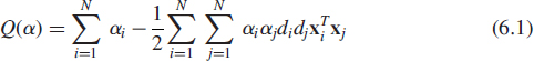
subject to the constraints

where α_i in (6.1) are the Lagrange multipliers, and the training data sample is denoted by with x_i denoting an input vector, d_i denoting the corresponding desired response, and N denoting the sample size.

Careful examination of (6.1) reveals essential ingredients of SVM learning, namely, the requirement to solve a quadratic programming problem, which can become a difficult proposition to execute in computational terms, particularly when the sample size N is large.

What we have addressed thus far is the optimal solution to a linearly separable pattern-classification problem. To extend the SVM learning theory to the more difficult case of nonseparable pattern-classification problems, a set of variables called slack variables are introduced into the convex optimization problem; these new variables measure the deviation of a point from the ideal condition of perfect pattern separability. It turns out that in mathematical terms, the impact of slack variables is merely to modify the second constraint in the dual optimization problem described in (6.1) as follows

where C is a user-specified positive parameter. Except for this modification, formulation of the dual optimization problem for nonseparable pattern-classification problems remains intact. Moreover, the support vectors are defined in the same way as before. The new parameter C controls the tradeoff between the complexity of the machine and the number of nonseparable patterns; it may therefore be viewed as the reciprocal of a parameter commonly referred to the regularization parameter. When parameter C is assigned a large value, the implication is that there is high confidence in the practical quality of the supervisory training data. Conversely, when C is assigned a small value, the training data sample is considered to be noisy, suggesting that less emphasis should be placed on its use and more attention be given to the adjustable parameter vector.

Thus far in the discussion, we have focused attention on an algorithmic formulation of the SVM. Clearly, we need a network structure for its implementation. In this context, the radial-basis function (RBF) provides a popular choice. Figure 6.3 depicts a structure of a RBF network, in which the nonlinear hidden layer of size K (smaller than the sample size N) consists of Gaussian units; nonlinearity of the hidden layer is needed to account for nonseparability of the input patterns. Each Gaussian unit is defined in terms of its m₀-dimensional center, where m₀ is the dimensionality of the input data space. To complete the specifications of the hidden layer, we need to define also the effective width of each Gaussian function acting as a receptive field. To simplify the network design, it is common practice to assign a common width to all the Gaussian units. As for the output layer, it is linear with m₁ adjustable parameters w₁, w₂, … w_m1, and an adjustable bias.

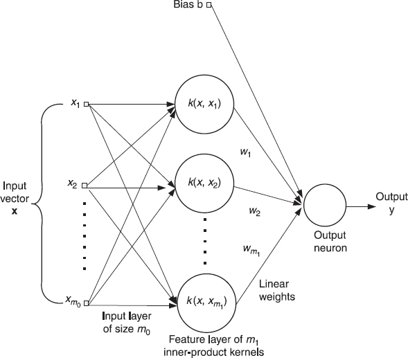
Figure 6.3 Architecture of support vector machine, using a radial basis function network.

To propose an application of the SVM algorithm to the RBF structure of Figure 6.3, we keep the following points in mind.

1. The support vectors picked out of the supervisory training data by the SVM algorithm define the centers of the Gaussian units in the hidden layer.
2. The outputs of the Gaussian units, produced in response to the data applied to the source (input) nodes of the RBF network, define the inputs applied to the adjustable parameters. In effect, x_i in (6.1) is now replaced by the vector

   

   where denotes the set of support vectors computed by the SVM algorithm. Thus, using (6.2) in (6.1), we see that the inner product in (6.1) is replaced by the new inner product

   

   which is called the Mercer kernel. This terminology follows from the fact that the functions assigned to the hidden units of the RBF network must satisfy the celebrated Mercer's theorem, which is indeed satisfied by the choice of Gaussian functions. Equation (6.3) provides the basis for the kernel trick, which states the following.

For this reason, a network structure exemplified by the RBF network, is referred to as a kernel machine and the SVM learning algorithm used to train it is referred to as a kernel method.

6.3 SUPERVISED TRAINING FRAMEWORK OF MLPs USING NONLINEAR SEQUENTIAL STATE ESTIMATION

To describe how a nonlinear sequential state estimator can be used to train a MLP in a supervised manner, consider a MLP with s synaptic weights and p output nodes. With n denoting a time-step in the supervised training of the MLP, let the vector w_n denote the entire set of synaptic weights in the MLP computed at time step n. For example, we may construct w_n by stacking the weights associated with neuron 1 in the first hidden layer on top of each other, followed by those of neuron 2, carrying on in this manner until we have accounted for all the neurons in the first hidden layer; then we do the same for the second and any other hidden layer in the MLP, until all the weights in the MLP have been accounted for in the vector w_n in the orderly fashion just described.

With sequential state estimation in mind, the state-space model of the MLP under training is defined by the following pair of models (see Fig. 6.4).

Figure 6.4 Nonlinear state-space model depicting the underlying dynamics of a MLP undergoing supervised training.

1. System (state) model, which is described by the first-order autoregressive equation

   

   The dynamic noise ω_n is white Gaussian noise of zero mean and covariance matrix Q_n which is purposely included in the system model to anneal the supervised training of the MLP over time. In the early stages of the training session, Q_n is large in order to encourage the supervised-learning algorithm to escape local minima, then it is gradually reduced to some finite but small value.

2. Measurement model, which is described by the equation

   

   where the new entities are defined as follows:

   • d_n is the vector denoting observables
   • u_n is the vector denoting the input signal applied to the network
   • v_n is the vector denoting the measurement noise process of zero mean and diagonal covariance matrix R_n. The source of this noise is attributed to the way in which d_n is actually obtained.

The vector-valued measurement function b (.,.) in (6.5) accounts for the overall non-linearity of the MLP from the input to the output layer; it is the only source of non-linearity in the state–space model of the MLP. Here, the notion of state refers to an externally adjustable state, which manifests itself in adjustments applied applied to the MLP's weights through supervised training—hence the inclusion of the weight vector w_n in the state-space model described by both (6.4) and (6.5).

6.4 THE EXTENDED KALMAN FILTER

Given the training sample , the issue of interest is how to undertake the supervised training of the MLP by means of a sequential state estimator. Since the MLP is nonlinear by virtue of the nonlinear measurement model of (6.5), the sequential state estimator would have to be correspondingly nonlinear. With this requirement in mind, we begin the discussion by considering how the extended Kalman filter (EKF) can be used to fulfil this rule.

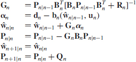
For the purpose of our present discussion, the relevant equations of the EKF algorithm summarized in Table 6.1 are the following two, using the terminology of the state–space model of (6.4) and (6.5).

1. The innovations process, defined by

   

   where the desired response d_n plays the role of the observable for the EKF.

   Table 6.1 Summary of the EKF algorithm for supervised training of the MLP

   Training sample: {un, dn}, n = 1, 2, … N where un is the input vector applied to the MLP and dn is the corresponding desired response. MLP and Kalman filter: Parameters and variables b(.,.) :    vector-valued measurement function B :    linearized measurement matrix wn :    weight vector at time step n ŵn|n−1 :    predicted estimate of the weight vector ŵn|n :    filtered estimate of the weight vector yn :    output vector of the MLP produced in response to un Qn :    covariance matrix of dynamic noise ωn Rn :    covariance matrix of measurement noise vn Gn :    Kalman gain Pn|n−1 :    prediction error covariance matrix Pn|n :    filtering error covariance matrix Initialization: The initial weights ŵ1|0 are drawn from a uniform distribution with zero mean and variance equal to the reciprocal of the number of synaptic connections feeding into a node (fan-in). The associated covariance of the initial weight estimate is fixed at δI, where δ can be ‘some’ multiples of 10, and I is the identity matrix. Recursive computation: For n = 1, 2, … compute the following:

2. The weight (state) update, defined by

   

   where ŵ_n|n−1 is the predicted (old) state estimate of the MLP's weight vector w at time n, given the desired response up to and including time (n − 1), and ŵ_n|n is the filtered (updated) estimate of w on the receipt of observable d_n. The matrix G_n is the Kalman gain, which is an integral part of the EKF algorithm.

Examining the underlying operation of the MLP, we find that the term b(ŵ_n|n−1, u_n) is the actual output vector y_n produced by the MLP with its old weight vector ŵ_n|n−1 in response to the input vector u_n. We may therefore rewrite the combination of (6.6) and (6.7) as a single equation:

On the basis of this insightful equation, we may now depict the supervised training of the MLP as the combination of two mutually coupled components that form a closed-loop feedback system, as shown in Figure 6.5.

1. The top part of the figure depicts the supervised learning process as viewed partly from the network's perspective. With the weight vector set at its old (predicted) value ŵ_n|n−1, the MLP computes the actual weight vector y_n as the predicted estimate of the observable—namely _n|n−1.
2. The bottom part of the figure depicts the EKF in its role as the facilitator of the training process. Supplied with _n|n−1 = y_n, the EKF updates the old estimate of the weight vector by operating on the current desired response d_n. The filtered estimate of the weight vector, namely, ŵ_n|n, is thus computed in accordance with (6.8). The EKF supplies ŵ_n|n to the MLP via a bank of unit-time delays.

With the transition matrix being equal to the identity matrix, as evidenced by (6.4), we may set ŵ_n+1|n equal to ŵ_n|n for the next iteration. This equality permits the supervised training cycle to be repeated until the training session is completed.

Note that in the supervised training framework of Figure 6.5, the training sample (u_n, d_n) is split between the MLP and the EKF: The input vector u_n is applied to the MLP as the excitation, and the desired response d_n is applied to the EKF as the observable, which is dependant on the hidden weight (state) vector w_n. From the predictor-corrector property of the Kalman filter and its variants and extensions, we find that examination of the block diagram of Figure 6.5 leads us to make the following insightful statement: The multilayer perceptron, undergoing training, performs the role of the predictor, and the EKF, providing the supervision, performs the role of the corrector. Thus, whereas in traditional applications of the Kalman filter for sequential state estimation, the roles of the predictor and corrector are embodied in the Kalman filter itself, in supervised training applications these two roles are split between the MLP and the EKF. Such a split of responsibilities in supervised learning is in perfect accord with the way in which the input and the desired response of the training sample are split in Figure 6.5.

Figure 6.5 Closed-loop feedback system embodying the MLP and the EKF: 1. The MLP, with weight vector ŵ_n|n−1, operates on the input vector u_n to produce the output vector y_n; 2. The EKF, supplied with the prediction _n|n−1 = y_n, operates on the current desired response d_n to produce the filtered weight estimate ŵ_n|n thereby preparing the closed-loop feedback system for the next iteration.

6.4.1 The EKF Algorithm

For us to be able to apply the EKF algorithm as the facilitator of the supervised learning task, we have to linearize the measurement equation (6.5) by retaining first-order terms in the Taylor series expansion of the nonlinear part of the equation. With b(w_n, u_n) as the only source of nonlinearity, we may approximate (6.5) as

where B_n is the p-by-s measurement matrix of the linearized model. The linearization process involves computing the partial derivatives of the p outputs of the MLP with respect to its s weights, obtaining the required matrix

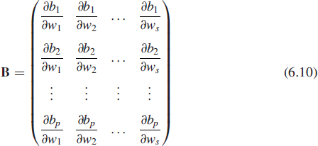
where b_i, i = 1, 2, … p, in (6.10) denotes the i-th element of the vectorial function b(.,.), and the partial derivatives on the right-hand side of (6.10) are evaluated at w_n = ŵ_n|n−1. Recognizing that the dimensionality of the weight vector w is s, it follows that the matrix product Bw is a p-by-1 vector, which is in agreement with the dimensionality of the observable d.

6.5 EXPERIMENTAL COMPARISON OF THE EXTENDED KALMAN FILTERING ALGORITHM WITH THE BACK-PROPAGATION AND SUPPORT VECTOR MACHINE LEARNING ALGORITHMS

In this section, we consider a binary class classification problem as shown in Figure 6.6(a). It consists of three concentric circles of radii 0.3, 0.8, and 1. It is a challenging problem because the two regions are disjoint and non-convex. For the experiment, we used the following supervised training algorithms

Figure 6.6 (a): Original; (b)–(d): Representative test classification results.

• MLP trained by the BP;
• MLP trained by the EKF; and
• RBF trained by the SVM.

The structure of the MLP was chosen to have two inputs, one output, and two hidden layers, with five neurons each. Hence, the MLP has a total of 51 adjustable parameters or weights (bias included). All neurons use the hyperbolic tangent function

The learning-rate parameter of the back-propagation algorithm was fixed at 0.01. For the MLPs trained by the BP and the EKF, the initial weights were set up as described in Section 6.4. For the EKF, two more covariance matrices were additionally required.

1. The covariance matrix of dynamic noise Q_n was annealed such that 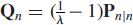, where P_n|n is the error covariance associated with the weight estimate at time instant n, and λ ∈ (0, 1) is the forgetting factor as defined in a recursive least-squares algorithm; this approximately assigns exponentially decaying weights to past observables; λ was fixed at 0.9995.
2. The variance of measurement noise R_n was fixed at unity.

For the SVM, the kernel in he RBF network was chosen to be the Gaussian radial-basis function. A kernel of width σ = 0.2 was found to be a good choice for this problem. This value was chosen based on the accuracy of test classification results. The soft margin of unity was found to be more appropriate for this problem. The quadratic programming code, available as an in-built routine in the MATLAB optimization toolbox, was used for training the SVM.

For the purpose of training 1000 data points were randomly picked from the considered region. In the MLP-based classification, each training epoch contained 100 examples randomly drawn from the training data set. For the purpose of testing, the test data were prepared as follows: A grid of 100 × 100 data points were chosen from the square region [−1, 1] × [−1, 1] [see Fig. 6.6(a)] and then the grid points falling outside the unit circle were discarded. In so doing, we were able to obtain 7825 test points.

At the end of every 10-training epoch interval, the MLP was presented with the test data set. We made 50 such independent experiment trials and the ensemble-averaged correct classification rate was computed. In contrast, for the SVM, this test grid was presented at the end of the training session. Figures 6.7(a) and 6.7(b) show the results of the BP-trained MLP and the EKF-trained MLP, respectively. At the end of 5000 training epochs, we obtained the following results: the BP-trained MLP achieves nearly 90 percent classification accuracy; whereas, at the end of 200 training epochs, the EKF-trained MLP achieves nearly 96 percent classification accuracy. Figures 6.6(b)–6.6(d) depict representative test classification results of the employed algorithms.

Figure 6.7 Ensemble-averaged (over 50 runs) correct classification rate versus number of epochs.

Table 6.2 Comparison of classification accuracy and computational times averaged over 50 independent experiments

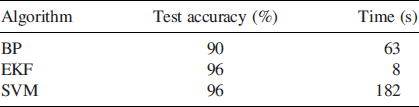
We also computed the computational times of each algorithm averaged over 50 independent trials when executing on an Intel Pentium Core Duo processor of cycle speed 2.1 GHz. The summarized results are presented in Table 6.2. To execute 5000 epochs of the BP, roughly a minute was required, whereas, the EKF required only 8 seconds for completing its 200 training epochs. As expected, the SVM was found to take more time (nearly 3 minutes) to complete its training session.

Based on the computational time-accuracy tradeoff, we may say that the EKF-trained MLP is the best choice for solving the difficult binary pattern-classification problem illustrated by Figure 6.6(a). Such a tradeoff may equally apply to other difficult pattern classification problems, and possibly large-scale ones.

6.6 CONCLUDING REMARKS

In the neural networks and learning machines literature, the solution to pattern-classification problems is commonly tackled, for example, by using a multilayer perceptron (MLP) trained with the back-propagation algorithm or a radial-basis function (RBF) network using the support-vector machine (SVM) learning algorithm [1]. In this chapter, we have discussed another way of tackling the pattern-classification problem, namely, a multilayer perceptron trained using the extended Kalman filter (EKF). The rationale for this unusual approach is that the supervised learning process, involving the training of a multilayer perceptron may be viewed as a state-estimation problem, in which case the weight vector characterizing the multilayer perceptron is viewed as a hidden state. An attractive feature of using the EKF for estimating the unknown weight vector is the improved utilization of the information contained in the training sample by propagating the covariance matrix of the filtered estimation error, hence the accelerated rate of learning. This point is borne out by the shorter time taken to complete the learning process, compared to both the BP and SVM algorithms. Moreover, the experimental results presented in Section 6.5 show that the EKF approach to the supervised training of a multilayer perceptron achieves a pattern-classification accuracy that matches the results obtainable with the SVM.

To conclude, we may say that the supervised training of a multilayer perceptron, using the EKF as the tool to oversee the supervision, deserves serious consideration when the requirement is to solve difficult, and possibly large-scale pattern-classification problems.

6.7 PROBLEMS

6.1  You are given a set of supervisory data samples of large enough size. The data are to be used for training of a learning machine, which is required to solve a difficult pattern-classification exemplified by that of Figure 6.6(a).

Describe the attributes of a learning machine that is required to tackle such pattern-classification problem.

6.2  Discuss the pros and cons of the extended Kalman filtering algorithm used to train a multilayer perceptron for solving the pattern-classification problem of Figure 6.6(a) compared to the back-propagation algorithm.

6.3  Repeat the experiment described in Section 6.5 to verify your conclusions in Problem 6.2.

6.4  Discuss the pros and cons of the extended Kalman filtering algorithm used to train a multilayer perceptron for solving the pattern-classification problem of Figure 6.6(a) compared to a radial-basis function network trained using the support vector machine (SVM) learning algorithm.

6.5  Repeat the experiment described in Section 6.5 to verify your conclusions in Problem 6.4.

6.6  The learning capability of the human brain extends beyond pattern-classification. To probe further, consider two people who love listening to music. One is in their mid-thirties, and the other is in their mid-sixties. Suppose a piece of music is being played on the radio some time in 2010: If the piece of music goes back to the 1970s, it is the second person who very much enjoys it. On the other hand, when the piece of music played on the same radio goes back to the 1990s, it is the first person who very much enjoys it.

Explain the main reason that is responsible for this difference.

REFERENCES

    1. S. Haykin, Neural networks and learning machines, 3rd ed., Prentice Hall, NJ, 2009.

    2. B. Schölkolf and A. J. Smola, Learning with kernels: Support vector machines, regularization, optimization, and beyond, MA: MIT Press, 2003.

    3. V. N. Vapnik, Statistical learning theory, NY: Wiley, 1998.