
In recent decades, a revolutionary change has taken place in the field of analytics technology because of big data. Data is being collected from a variety of sources, so technology has been developed to analyze this data in a distributed environment, even in real time.
Hadoop
The revolution started with the development of the Hadoop framework, which has two major components, namely, MapReduce programming and the HDFS file system.
MapReduce Programming
MapReduce is a programming style inspired by functional programming to deal with large amounts of data. The programmer can process big data using MapReduce code without knowing the internals of the distributed environment. Before MapReduce, frameworks like Condor did parallel computing on distributed data. But the main advantage of MapReduce is that it is RPC based. The data does not move; on the contrary, the code jumps to different machines to process the data. In the case of big data, it is a huge savings of network bandwidth as well as computational time.
A MapReduce program has two major components: the mapper and the reducer. In the mapper, the input is split into small units. Generally, each line of input file becomes an input for each map job. The mapper processes the input and emits a key-value pair to the reducer. The reducer receives all the values for a particular key as input and processes the data for final output.
Partitioning Function
Sometimes it is required to send a particular data set to a particular reduce job. The partitioning function solves this purpose. For example, in the previous MapReduce example, say the user wants the output to be stored in sorted order. Then he mentions the number of the reduce job 32 for 32 letters, and in the practitioner he returns 1 for the key starting with a, 2 for b, and so on. Then all the words that start with the same letters go to the same reduce job. The output will be stored in the same output file, and because MapReduce assures that the intermediate key-value pairs are processed in increasing key order, within a given partition, the output will be stored in sorted order.
Combiner Function
The combiner is a facility in MapReduce where partial aggregation is done in the map phase. Not only does it increase the performance, but sometimes it is essential to use if the data set so huge that the reducer is throwing a stack overflow exception. Usually the reducer and combiner logic are the same, but this might be necessary depending on how MapReduce deals with the output.
To implement this word count example, we will follow a particular design pattern. There will be a root RootBDAS (BDAS stands for Big Data Analytic System) class that has two abstract methods: a mapper task and a reducer task. All child classes implement these mapper and reducer tasks. The main class will create an instance of the child class using reflection, and in MapReduce map functions call the mapper task of the instance and the reducer function of the reducer task. The major advantages of this pattern are that you can do unit testing of the MapReduce functionality and that it is adaptive. Any new child class addition does not require any changes in the main class or unit testing. You just have to change the configuration. Some code may need to implement combiner or partitioner logics. They have to inherit the ICombiner or IPartitioner interface.

A flow diagram illustrates how the main class, unit tester, and child 1 and 2 are linked to classes of abstract and interfaces.
The class diagram
HDFS File System
Other than MapReduce, HDFS is the second component in the Hadoop framework. It is designed to deal with big data in a distributed environment for general-purpose low-cost hardware. HDFS is built on top of the Unix POSSIX file system with some modifications, with the goal of dealing with streaming data.
The Hadoop cluster consists of two types of host: the name node and the data node. The name node stores the metadata, controls execution, and acts like the master of the cluster. The data node does the actual execution; it acts like a slave and performs instructions sent by the name node.
MapReduce Design Pattern
MapReduce is an archetype for processing the data that resides in hundreds of computers. There are some design patterns that are common in MapReduce programming.
Summarization Pattern

A flow diagram illustrates how the mapper, partitioner, and reducer are linked through key, summary field, groups, and summary.
Details of the summarization pattern
Filtering Pattern
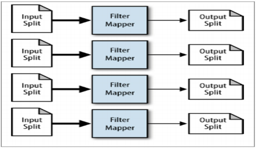
A flow diagram illustrates how the four frames of input splits are connected to their respective output splits through filter mappers.
Details of the filtering pattern
Join Patterns

A flow diagram illustrates how mappers 1 and 2 are connected to a common reducer to predict the output of key, and values 1 and 2.
Details of the join pattern
A Notes on Functional Programming
MapReduce is functional programming. Functional programming is a type of programming in which all variables are immutable, making parallelization easy and avoiding race conditions. Normal Python allows functional programming.
Spark

A block diagram lists the components of the spark core as spark S Q L structured data, spark streaming real-time, M Lib machine learning, Graph X, scheduler, YARN, and Mesos.
The components of Spark
Spark Core is the fundamental component of Spark. It can run on top of Hadoop or stand-alone. It abstracts the data set as a resilient distributed data set (RDD). RDD is a collection of read-only objects. Because it is read-only, there will not be any synchronization problems when it is shared with multiple parallel operations. Operations on RDD are lazy. There are two types of operations happening on RDD: transformation and action. In transformation, there is no execution happening on a data set. Spark only stores the sequence of operations as a directed acyclic graph called a lineage. When an action is called, then the actual execution takes place. After the first execution, the result is cached in memory. So, when a new execution is called, Spark makes a traversal of the lineage graph and makes maximum reuse of the previous computation, and the computation for the new operation becomes the minimum. This makes data processing very fast and also makes the data fault tolerant. If any node fails, Spark looks at the lineage graph for the data in that node and easily reproduces it.
Spark SQL, which is a SQL interface through the command line or a database connector interface. It also provides a SQL interface for the Spark data frame object.
Spark Streaming, which enables you to process streaming data in real time.
MLib, a machine learning library to build analytical models on Spark data.
GraphX, a distributed graph processing framework.
PySpark
- 1.
First, we need Java Runtime Environment (JRE) in order to run Spark. It is recommended to install JRE from following link: https://adoptium.net/temurin/releases/?version=8. Also, you can install JRE from other distribution.
The installation will automatically create JAVA_HOME. If it does not, we need to set JAVA_HOME as the system variable; the value should be the location of the Java installation folder such as JAVA_HOME=C:Program FilesEclipse Adoptiumjdk-8.0.345.1-hotspot.
- 2.
Then we need to install PySpark using the command pip install pyspark.
For this we need to have Python 3.7 and above installed. After that, we need to set env PYSPARK_PYTHON as the location of Python. Here’s an example: C:Users...ProgramsPythonPython39python.exe.
- 3.
Also, install PyArrow by using pip install pyarrow to use the Pandas API in PySpark.
Updatable Machine Learning and Spark Memory Model
In this section, we discuss a new machine learning topic: how to develop an updatable machine learning model, which is a basic requirement for a model to become scalable.
When we train a model in machine learning, we data train the model from scratch, which implies that all the information from prior training iterations is swapped out. For example, if we train a model with data from the first week of the month, it will predict based on the first week’s data, and if we train the same model object with data from the second week, it will predict based on the second week’s data. It begins to forecast based only on data from the second week of the month. In the model, there is no trace of first-week data. However, in the real world, there are many scenarios when we require the model to forecast based on first- and second-week data after training, which implies that each training iteration will update the model rather than erase prior training information.
This type of model is possible when the model is a function of X and for any two data sets N1 and N2.
X(N1) + X(N2) = X(N1+N2)
Examples of this type of function are count, max, min, and sum. Any probability-based model may be divided into sum and count and therefore converted into an updatable model. The Bayesian classifier was used as a model in our application, and the Spark code in the next is our own implementation of the classifier.
The algorithm’s goal is to determine the conditional probability that a Node(video or content) will be observed for a specific feature value.
Feature count = Number of records where that device ID (49) is present
Conditional count = Number of records with is_completed equal to 1, identifier equal to 49, and node equal to 10033207
The ratio of the conditional count and feature count will represent the actual probability, but we are not dividing this stage because the model will not be updatable.
- 1.
Create a user-defined function to convert the IP address to geographic locations.
- 2.
Read the name of the target channel from the config file.
- 3.
In a data frame, load the lines from the application server log except for the line that contains the newlog.
- 4.
Filter the logline that includes the channel name.
- 5.
Read important column names from the config and selecting them from the data frame.
- 6.
Connect to MySQL and reading the threshold timestamp from the threshold table.
- 7.
In MySQL, filter the data frame column with a timestamp more than the threshold, get the max timestamp from the selected logline, and set that as the new threshold for the next iteration.
- 8.
The content or node IDs that are clicked are then saved in the database.
- 9.
Store the popular contents or node in the database.
- 10.
Each line contains the user’s next watch node, which is obtained by self-joining the user’s previous watch node.
- 11.
Then calculate the ratio of watch time and duration of video as a score.
- 12.
If the score is greater than the channel’s threshold defined in config, mark it 1; otherwise, mark it 0.
- 13.
Then, as stated in Chapter 3, calculate the conditional probability of a user watching a video that is longer than the threshold in the form of a count.
We will discuss something crucial about the Spark memory model now. The operation is performed in memory by Spark. Using a command-line parameter, we can change the default size of execution memory. Spark can handle files that are greater than its RAM, but it must use disc memory to do it. For example, the input log file was greater than the Spark memory size, but the program successfully filters important lines from there. However, there is one exception. If you do decide to join, Spark requires the memory of both data frames. We use a join here to make our code as memory-optimized as possible by manually calling the Spark garbage collector via the unpersist function. However, it slows down the code. If you eliminate that code, the program will run faster but use more memory.
Analytics in the Cloud
Like many other fields, analytics is being impacted by the cloud. It is affected in two ways. Big cloud providers are continuously releasing machine learning APIs. So, a developer can easily write a machine learning application without worrying about the underlining algorithm. For example, Google provides APIs for computer vision, natural language, speech processing, and many more. A user can easily write code that can give the sentiment of an image of a face or voice in two or three lines of code.
The second aspect of the cloud is in the data engineering part. In Chapter 1 we gave an example of how to expose a model as a high-performance REST API using Falcon. Now if a million users are going to use it and if the load varies by much, then auto-scale is a required feature of this application. If you deploy the application in the Google App Engine or AWS Lambda, you can achieve the auto-scale feature in 15 minutes. Once the application is auto-scaled, you need to think about the database. DynamoDB from Amazon and Cloud Datastore by Google are auto-scaled databases in the cloud. If you use one of them, your application is now high performance and auto-scaled, but people around globe will access it, so the geographical distance will create extra latency or a negative impact on performance. You also have to make sure that your application is always available. Further, you need to deploy your application in three regions: Europe, Asia, and the United States (you can choose more regions if your budget permits). If you use an elastic load balancer with a geobalancing routing rule, which routes the traffic from a region to the app engine of that region, then it will be available across the globe. In geobalancing, you can mention a secondary app engine for each rule, which makes your application highly available. If a primary app engine is down, the secondary app engine will take care of things.

A flowchart lists the elastic load balancer. It has system instances 1, 2, and 3 with primary as Asia, U S, and Europe and secondary as U S, Europe, and Asia.
The system
- 1.
The ad server requests an impression prediction.
- 2.
When the main thread receives the request predictor, it creates a new thread for each feature.
- 3.
By sending a concurrent request to the data store, each thread calculates is big, floor, floor big, probability, and probability big for each feature. It returns 0 if the feature or value is not found in the data store.
- 4.
If is big indicates a high-value impression, large scores are used; otherwise, general scores are used.
- 5.
It predicts score = ∑ score for each feature.
- 6.
It calculates the final predicted floor using the multiplier range obtained from the data store.
- 7.
The predicted floor value is returned to the ad server in the response.
Internet of Things
The IoT is simply the network of interconnected devices embedded with sensors, software, network connectivity, and necessary electronics that enable them to collect and exchange data, making them responsive. The field is emerging with the rise of technology just like big data, realtime analytics frameworks, mobile communication, and intelligent programmable devices. In the IoT, you can analyze data on the server side using the techniques shown throughout the book; you can also put logic on the device side using the Raspberry Pi, which is an embedded system version of Python.
Essential Architectural Patterns for Data Scientists
Data is not an isolated entity. It must gather data from some application or system, then store it accurately in certain storage, and then construct a model on top of that model, which must then be provided as an API to connect with other systems. This API must occasionally be present throughout the world with a certain latency. So, much engineering goes into creating a successful intelligent system, and in today’s startup environment, which is a multibillion-dollar industry, an organization cannot afford to hire a large number of specialists to create a unique feature in their product. In the startup world, the data scientist must be a full-stack analytic expert. So, in the following sections, we’ll provide different scenarios with Tom, a fictitious character, to illustrate several key architectural patterns that any data scientist should be aware of.
Scenario 1: Hot Potato Anti-Pattern
Tom is employed as a data scientist to work on a real-time analytics product for an online company. So, the initial step is to gather data from his organization’s application. They use the cloud to auto-scale their storage, and they push data straight to the database from the application. In the test environment, everything appears to be in order. To ensure that there is no data loss, they use a TCP connection. When they go live, though, they do not make any changes to the main application, and it crashes. The company faces a massive loss within a half-hour, and Tom gets real-time feedback for his first step of the real-time analytic system: he is fired.
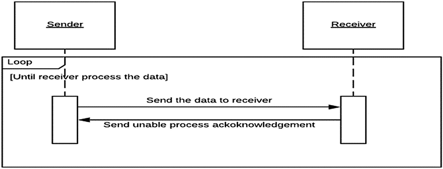
A diagram illustrates how the sender sends the data to the receiver, which in turn, gives the unable process acknowledgment to the sender in a loop.
Sequence diagram describing Hot Potato anti-pattern
There are two elements to the situation. If the data that passes between the sender and the recipient is not required, we can use the UDP protocol, which drops the data that is unable to deliver. It’s one of the factors why UDP is used in all network monitoring protocols, such as SNMP and NetFlow. It does not require the device to be loaded to monitor. However, if the data is essential, such as in the financial industry, we must create a messaging queue between the sender and the recipient. When the receiver is unable to process data, it functions as a buffer. If the queue memory is full, the data is lost, or the load is transferred to the sender. ZMQ stands for “zero message queues,” and it’s nothing more than a UDP socket.
In cloud platforms, there are numerous readymade solutions; we go through them in depth in Chapter 2. The following Node.js code shows an example of a collector that uses Rabit-MQ and exposes it as a REST API to the sender, using Google Big Query as the receiver.
Code: Data Collector Module
Now, let’s explore other important architectural patterns, proxy and layering.
Scenario 2: Proxy and Layering Patterns
Tom starts working at a new company. There is no job uncertainty because the company is large. He does not take the risk of gathering the data in this case. The data is stored on a MySQL server. Tom had no prior knowledge of the database. He was passionate about learning MySQL. In his code, he writes lots of queries. The database is owned by another team, and their manager likes R&D. So every Monday, Tom receives a call informing him that the database has changed from MySQL to Mongo and subsequently from Mongo to SQL Server, requiring him to make modifications across the code. Tom is no longer unemployed, but he returns home from work every day at midnight.
Everyone seems to agree that the solution is to properly arrange the code. However, understanding the proxy and layering patterns is beneficial. Instead of utilizing a raw MySQL or Mongo connection in your code, employ a wrapper class as a proxy in the proxy pattern. Using the layering technique, divide your code into many layers, each of which uses a method exclusively from the layer below it. Database configuration should be done at the lowest levels, or core layer, in this instance. Above that is the database utility layer, which includes the database queries. Above that, there is a business entity layer that makes use of database queries. The following Python code will help you see things more clearly. Tom now knows that if there are any changes at the database level, he must investigate the core layer; if there are any changes in queries, he must investigate the database utility layer; and if there are any changes in business actors, he must investigate the entity layer. As a result, his life is now simple.
Database Core Layer
Thank You
We would thank you for reading this book. We hope you have enjoyed reading the book as we much as enjoyed writing it. We hope it helps you make a footprint on machine learning community. We would like to encourage you to keep practicing on different data sets and contribute to the open-source community. You can always contact us through the publisher. Thank you once again and best wishes!