Help and Documentation

The R community has many resources to help users. From prebuilt functions to whole collections of themed functions in packages, there are many types of support. Both ? and help are useful ways to access information about an object or function. For more common objects, R has not only extensive documentation about specifics such as input (for functions), but also detailed notes on what those inputs are expected to receive. Furthermore, often detailed examples showcase just what can be done. Figure 2-1 shows the output of using these two functions with the addition operator :

Figure 2-1. Help documentation for arithmetic operators

?'+'              
help("+")              

Notice at the bottom of Figure 2-1 that the documentation for arithmetic operators is even kind enough to provide specific information about the fact that there can be differences in output depending on the platform. It is important to note that not all functions have this fully complete documentation readily available, but for many of the most common functions and packages, an extraordinary level of information is available. Writing code that reproduces the desired results, independent of platform and environment, is not always possible. Later, when we discuss debugging, it is this sort of advanced knowledge of various functions that can be helpful to know.

Of course, this kind of help is more useful when you already know the object or function you want to use and simply need more details. When seeking the ability to do something entirely new, referring to the manuals can help. One such site is https://cran.r-project.org/manuals.html maintained by the R Development Core Team.

We turn our attention now to the ways that R can access system files.

System and Files

In a Windows environment, R may be a very effective way to automate file manipulation. Most IT departments are willing to install R, and it has the same file permission privileges you do. From creating files to moving them about and checking dates, R has a variety of functions that are handy for getting information from the system and automating file management . Our observation is that Unix-based systems might have more-elegant ways of handling such scenarios from the command line.

One helpful feature of R accessing the system is that it is possible to discover the current date, time, and time zone of the system on which R is being run. This can help detect new files or can be used to put timestamps into files (more on that later). It should be noted that these are, of course, dependent on the system environment being accurate, so caution may be in order before using these in high-stakes projects .

Sys.Date()                
[1] "2016-02-13"

Sys.time()                
[1] "2016-02-13 16:58:36 CST"

Sys.timezone()                
[1] "America/Chicago"

The help documentation for these commands makes useful suggestions to increase the accuracy of the output, up to potentially millisecond or microsecond precision.

Let’s turn our attention now to a variety file management functions. These all share the format file.* and have as their first argument a character vector that should be either a filename for the current working directory or a path and filename. We start with a text file ch02_text.txt in our working directory.

The function file.exists()takes only a character string input, which is a filename or a path and filename. If it is simply a filename, it checks only the working directory. This working directory is verified by the getwd()function. If a check is desired for a file in another directory, this may be done by giving a full file path inside the string. This function returns a logical value of either TRUE or FALSE. Depending on user permissions for a particular file, you may not get the expected result for a particular file.

 getwd()              
[1] "C:/Books/Apress_AdvancedR/RFiles"
 file.exists("ch02_text.txt")              
[1] TRUE
 file.exists("NOSUCHFILE.FAKE")              
[1] FALSE
 file.exists("C:/Books/Apress_AdvancedR/Apress_AdvancedR_Proposal.docx")              
[1] TRUE

While the preceding function checks for existence, another function tests for whether we have access to a file. The function file.accesstakes similar input, except it also takes a second argument. To test for existence, the second argument is 0. To test for executable permissions, use 1; and to test for writing permission, use 2. If you want to test your ability to read a file, use 4. This function returns an integer vector of 0 to indicate that permissions are given, and -1 to indicate permissions are not given. Notice that the default for the function is to test for simple existence. Examples of file.access are shown here:

file.access("ch02_text.txt")              
ch02_text.txt
            0
file.access("ch02_text.txt", mode = 0)              
ch02_text.txt
            0
file.access("ch02_text.txt", mode = 1)              
ch02_text.txt
           -1
file.access("ch02_text.txt", mode = 2)              
ch02_text.txt
            0
file.access("ch02_text.txt", mode = 4)              
ch02_text.txt
            0

We next turn our attention to more detailed information about when a file was modified, changed, or accessed with the file.info function . This function takes in character strings as well. The output gives information about the file size; whether it is a directory; a file permissions integer in read, write, and execute order; the last modified time; the last change time; the last accessed time; and finally, whether the file is executable:

file.info("ch02_text.txt", "chapter01.R")              
              size isdir mode               mtime               ctime               atime exe
ch02_text.txt   31 FALSE  666 2016-02-13 17:00:16 2016-02-13 16:59:57 2016-02-13 16:59:57  no
chapter01.R   7983 FALSE  666 2016-01-01 02:53:17 2016-01-05 12:26:39 2016-01-01 02:53:17  no

Notice that you can edit the modified time through the sys.setFileTime function . This can be helpful on occasion, although the precise accuracy and precision are dependent on the environment. Here’s an example:

newTime<-Sys.time()-20                
newTime                
[1] "2016-02-13 20:25:53 CST"

file.info("ch02_text.txt")                
              size isdir mode               mtime               ctime               atime exe
ch02_text.txt   31 FALSE  666 2016-02-13 17:00:16 2016-02-13 16:59:57 2016-02-13 16:59:57  no

Sys.setFileTime("ch02_text.txt", newTime)                
file.info("ch02_text.txt")                
              size isdir mode               mtime               ctime               atime exe
ch02_text.txt   31 FALSE  666 2016-02-13 20:25:53 2016-02-13 16:59:57 2016-02-13 16:59:57  no

Turning our attention to creation and removal of files, the functions file.createand file.removedo precisely what you would hope. These do return logically TRUE or FALSE and can even give more details:

file.create("ch02_created.docx", showWarnings = TRUE)              
[1] TRUE
file.remove("ch02_created.docx")              
[1] TRUE
file.remove("NOSUCHFILE.FAKE")              
[1] FALSE
Warning message:
In file.remove("NOSUCHFILE.FAKE") :
 cannot remove file 'NOSUCHFILE.FAKE', reason 'No such file or directory'

Files may also be copied and renamed. The function file.copycan be given overwrite permission, and could even be set up to copy entire folders and subfolders with the recursive=TRUE option . Furthermore, it has options to copy over mode or file permissions as well as to copy the file date data (or, of course, letting the copy have a new modified date). The following code example shows how that might all work:

Sys.time()              
[1] "2016-02-13 21:05:29 CST"
file.copy("ch02_text.txt", "ch02_copy.txt", overwrite = TRUE, recursive = FALSE, copy.mode = TRUE, copy.date = TRUE)              
[1] TRUE
file.info("ch02_copy.txt")              
              size isdir mode               mtime               ctime               atime exe
ch02_copy.txt   31 FALSE  666 2016-02-13 20:25:53 2016-02-13 21:05:30 2016-02-13 21:05:30  no
file.rename("ch02_copy.txt", "ch02.txt")              
[1] TRUE

The file.append function joins two files together. This can work well for some files types. Used naively, there can be unfortunate consequences. While the code to perform this follows, pay careful attention to Figure 2-2 and Figure 2-3. In the case of the text files, the process worked well enough. In the case of Microsoft PowerPoint files, not so much. Keep in mind that the PowerPoint files are less about the files themselves (neither author imagines using R for such files genuinely), and more about the fact that the nuances of file manipulation, in general, deserve treatment with due caution. Notice that R believes both operations are successful:

Figure 2-2. The first operation was successful according to R and worked upon opening the file

Figure 2-3. The second operation was successful according to R yet did not work upon opening the file

file.append("ch02_text.txt", "ch02.txt")              
[1] TRUE
file.append("ch02_pp.pptx", "ch02_pp2.pptx")              
[1] TRUE

You can not only manipulate files with R, but also create directories, or file folders, as well. The function is dir.create, which behaves as you might now expect. We show an example of the function here, and the resulting director in Figure 2-4:

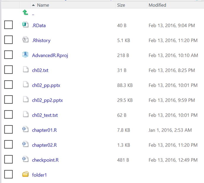
Figure 2-4. The created folder1 directory

dir.create("folder1")              

These commands work on any files that a user has permission to access and manipulate. One of the authors uses these commands to move data from various shared drives owned by different departments to eventually post result files on a website. Once you understand loops and functions from future chapters, you’ll be able to automate most file management.

Input

Getting new data into R becomes the next challenge. Data sets tend to be quite large, although effective techniques may be used on smaller sets. Text files with tab or comma separation are the most straightforward to import into R. Next, common data file types include Microsoft Excel, SPSS, SAS, and Stata. More generally, it is fairly safe to say that there likely exists an R package that can handle the type of file import you want. Even PDF and Microsoft Word files may be input should the need arise (text analytics from word clouds to more predictive applications come to mind). For most of these records, the input process is similar, so there is perhaps less of a need to be exhaustive and more of a need to set up sound principles. Be sure to visit the Apress website for this text to download the code packets for this book. We use files in the chapter 02 folder in our next examples; the Counties in Illinois files (All Counties in Illinois, 2016) and the rscfp2013 files (DADS, 2016) are used.

We start with a function in R, read.table(), which can take in several of the more basic file types and read them in as a data frame. As with most input functions, this has several options, not all of which are required for any particular circumstance. Depending on the type of data read into R, it may take more than one try to successfully read in the data in a way convenient to use and manipulate. The View function can be of help in this case, with the output shown in Figure 2-5.

Figure 2-5. The output of the View() function

countiesILCSV<-read.table("Ch02/Counties_in_Illinois.csv", header = TRUE, sep = ",")              
View(countiesILCSV)              

We use three packages—Hmisc (Harrell, 2016), xlsx (Dragulescu, 2014), and foreign (R Core Team, 2015)—to showcase input from various file types. One observation is that file types may, in fact, be quite large. With over 30,000 entries, as shown in Figure 2-6, read.dta quickly and handily imports Stata files .

Figure 2-6. A larger Stata .dta file successfully imported into R with thousands of entries

library(checkpoint)              
checkpoint("2016-09-04", R.version = "3.3.1")              
library(Hmisc)              
library(foreign)              
library(xlsx)              
rscfpData <- read.dta("Ch02/rscfp2013.dta")              
View(rscfpData)              

We can also import SPSS files through the spss.get function. Even if there are warnings, it can often be the case that data is still successfully imported. If the data is not imported successfully, search the warning message for specifics. In this case, it seems from our header view that all is well. For brevity’s sake, we truncated part of the header output:

countiesILSPSS <- spss.get("Ch02/Counties_in_Illinois.sav")                
Warning message:
In read.spss(file, use.value.labels = use.value.labels, to.data.frame = to.data.frame,  :
  Ch02/Counties_in_Illinois.sav: Unrecognized record type 7, subtype 18 encountered in system file

head(countiesILSPSS)                
                   county.name total.population median.income
1 Adams County, Illinois                  67030         43824
2 Alexander County, Illinois               8449         28833
3 Bond County, Illinois                   17904         51946
4 Boone County, Illinois                  53567         61210
5 Brown County, Illinois                   6897         38696
6 Bureau County, Illinois                 35083         45692
  less.than.high.school high.school some.college bachelors.or.higher
1            0.06938496   0.3663752    0.3155484          0.24869141
2            0.17821309   0.3999044    0.3251314          0.09675108
3            0.08590590   0.3386204    0.3054077          0.27006600
4            0.12358696   0.3577536    0.2985507          0.22010870
5            0.24846045   0.3012790    0.3270962          0.12316438
6            0.09044028   0.3910391    0.3542198          0.16430076

We’ll do one final example with Excel, which uses our last package, xlsx. This package has rJava (Urbanek, 2016) as a dependency, and that is relevant depending on which R version you use. Your mostly fearless authors stick to 64-bit as often as possible, and this requires a 64-bit version of Java installed. R was liberal with its complaints when this had not been done. Notice that sheet names can be specifically called, making the function read.xlsx handy for extracting specific pieces of data.

countiesILExcel <- read.xlsx("Ch02/Counties_in_Illinois.xlsx", sheetName = "Counties_in_Illinois")              

These three packages, along with R’s more inherent ability to read in tabular data stored in text files with various delimiters, allow for easy enough input of most data that might be presorted or collected. It is not difficult to direct R to look directly online for files either, so that one researcher may update records and those results can be readily percolated to others. Later, as part of other examples, we have some files that are downloaded live from the Internet. For now, we turn our attention to output.

Output

Output comes in many forms. Perhaps because of collaboration with other researchers or partners, accommodating one of the other software systems is needed. Much like the preceding section on input, R can readily output to several file types. Of more interest is setting up R to send specific console output to certain files. This allows one machine to view the results of an analysis run on another computer. In this section, we demonstrate a couple of outputs of data to SPSS, Stata, and Excel. Then we work with console outputs. We ask you to keep in mind that there are many other ways and types of files to create, and as part of larger examples, we demonstrate several types including various document files and graphics.

To output files to Excel, SPSS, or Stata, simply use the correct invocation of either the xlsx or foreign packages. As shown in Figure 2-7, R creates the output handily.

Figure 2-7. Output in Excel, SPSS , and Stata file formats is created from R

write.xlsx(countiesILExcel, "Ch02/Output1.xlsx")                

write.foreign(countiesILExcel, "Ch02/Output2.txt", "Ch02/Output2.sps",   package="SPSS")                
Warning message:
In writeForeignSPSS(df = list(county_name = c(1L, 2L, 3L, 4L, 5L,  :
  some variable names were abbreviated

write.dta(countiesILExcel, "Ch02/Output3.dta")                
Warning message:
In write.dta(countiesILExcel, "Ch02/Output3.dta") :
  abbreviating variable names

The sink function takes console output and directs it to a file. Thus, the results of an R process may be stored for later observation or saved to a shared drive for perusal by others. The console sends only output to the file, not the input. Look carefully at the difference between the code that follows and the screenshot of Output4.txt shown in Figure 2-8:

Figure 2-8. The output of the sink() function to a text file

sink("Ch02/Output4.txt", append = TRUE, split = TRUE)              
x <- 10              
xSquared <- x^2              
x              
[1] 10
xSquared              
[1] 100
unlink("Ch02/Output4.txt")              

We turn our attention away from the output for a little while, knowing that we’ll revisit this topic in several more chapters. Output of various types are necessary, and they tend to depend on objectives and circumstances.

The next chapter provides tools for quickly repeating similar operations again and again as well as handling course corrections based on the environment. Those techniques combine with these methods to quite handily automate file management on a relatively large scale.

References

References are given once and not repeated for packages. Data files found online are cited when used. Our goal is to give credit where it is due, without overloading the text.