We already briefly introduced the data.table package. This package is the heart of this chapter, which covers the basics of accessing, editing, and manipulating data under the broad term data management. Although not glamorous, data management is a critical first step to data visualization or analysis. Furthermore, the majority of time on a particular analysis project may come from the data management. For example, running a linear model in R can take one line of code, once the data is clean and in the format that the lm() function in R expects. Data management can be challenging, because raw data come in all types, shapes, and formats; missing data is common; and you may also have to combine or merge separate data sources. In this chapter, we introduce both mechanical and philosophical techniques to approach data management. All packages used in this chapter are already in our checkpoint.R file. Thus you need only source the file to get started.
In this chapter, we use the data.table R package (Dowle, Srinivasan, Short, and Lianoglou, 2015). The following code loads the checkpoint (Microsoft Corporation, 2016 ) package to control the exact version of R packages used and then loads the data.table package:
## load checkpoint and required packageslibrary(checkpoint)checkpoint("2016-09-04", R.version = "3.3.1")library(data.table)options(width = 70) # only 70 characters per line
Introduction to data.table
One of the benefits of using data tables, rather than the built-in data frame class objects , is that data tables are more memory efficient and faster to manipulate and modify. The data.table package accomplishes this to a large extent by altering data tables in place in memory, whereas with data frames, R typically makes a copy of the data, modifies it, and stores it. Making a full copy happens regardless of whether all columns of the data are being changed or, for example, 1 of 100 columns. Consequently, operations on data frames tend to take more time and use up more memory than comparable operations with data tables. To show the concepts of data management, we work with small data, so memory and processor time are not an issue. However, we highlight the use of data tables, rather than data frames, because data tables scale gracefully to far larger amounts of data than do data frames. There are other benefits of data tables as well, including not requiring all variable names to be quoted, that we show throughout the chapter. In contrast, the major advantage of data frames is that they live in base R, and more people are familiar with working with them (which is helpful, for example, if you share your code).
Data tables can be quite large. Rather than viewing all your data, it is often helpful to view just the head() and the tail(). When you show a data table in R by typing its name, the first and last five rows are returned by default. R also defaults to printing seven significant digits, which can make our numerical entries messy. For cleanness, we use the options() function to control some of the global options so that only the first and last three rows print (if the data table has more than 20 rows total—otherwise, all are shown); in addition, only two significant digits display for our numerical entries. While we set this, we also introduce Edgar Anderson’s iris data. This data involves sepal and petal lengths and widths in centimeters of three species of iris flowers.
Before we convert the iris data into a data table, we are going to convert our species’ names to a character rather factor class. In the following code, we set our options, force the species’ names to characters, and create our data table, diris:
options(stringsAsFactors = FALSE,datatable.print.nrows = 20, ## if over 20 rowsdatatable.print.topn = 3, ## print first and last 3digits = 2) ## reduce digits printed by Riris$Species <- as.character(iris$Species)diris <- as.data.table(iris)dirisSepal.Length Sepal.Width Petal.Length Petal.Width Species1: 5.1 3.5 1.4 0.2 setosa2: 4.9 3.0 1.4 0.2 setosa3: 4.7 3.2 1.3 0.2 setosa---148: 6.5 3.0 5.2 2.0 virginica149: 6.2 3.4 5.4 2.3 virginica150: 5.9 3.0 5.1 1.8 virginica
There are 150 rows of data comprising our three species: setosa, versicolor, and virginica. Each species has 50 measurement sets. R lives in memory, and for huge data tables, this may cause issues. The tables() command shows all the data tables in memory, as well as their sizes. In fact, tables() is itself a data table. Notice that the function gives information as to the name of our data table(s), the number of rows, columns, the size in MB, and if there is a key. We discuss data tables with a key in just a few paragraphs. For now, notice that 1MB is not likely to give us memory issues:
tables()NAME NROW NCOL MB[1,] diris 150 5 1COLS KEY[1,] Sepal.Length,Sepal.Width,Petal.Length,Petal.Width,SpeciesTotal: 1MB
If we need more information about the types of data in each column, calling the sapply()command on a data table of interest along with the class() function works. Recall that the *apply functions return results from calling the function named in the second formal on the elements from the first formal argument. In our case, class() is called on diris, and we see what types of values are stored in the columns of diris:
sapply(diris, class)Sepal.Length Sepal.Width Petal.Length Petal.Width Species"numeric" "numeric" "numeric" "numeric" "character"
Data tables have a powerful conceptual advantage over other data formats. Namely, data tables may be keyed. With a key, it is possible to use binary search. For those new to binary search, imagine needing to find a name in a phone book. It would take quite some time to read every name. However, because we know that the telephone directory sorts alphabetically, we can instantly find a middle-of-the-alphabet name, determine whether our search name belongs before or after that name, and remove half the phone book from our search in the process. Our algorithm may be repeated with the remaining half, leaving only a quarter of the original data to search after just two accesses! More mathematically, while a search through all terms of a data frame would be linear based on the number of rows, n, in a data table, it is at worse log n. In a few new tables we, the authors, used, doubling our data added only minutes to code runtime rather than doubling runtime. A major win.
Note
In data.table, a key is an index that may or may not be unique, created from one or more columns in the data. The data is sorted by the key, allowing very fast operations using the key. Example operations include subsetting or filtering, performing a calculation (for example, the mean of a variable) for every unique key value, and merging two or more data sets.
Of course, it does take time to key a data table, so it depends on how often you access your data before making this sort of choice. Another consideration is what to use as the key. A table has only one key, although that key consist of more than one column. The function setkey()takes a data table as the first formal and then takes an unspecified number of column names after that to set a key. To see whether a data table has a key, simply call haskey() on the data table you wish to test. Finally, if you want to know what columns built the key, the function key() called on the data table provides that information. We show these commands on our data table diris in the following code lines:
haskey(diris)[1] FALSEsetkey(diris, Species)key(diris)[1] "Species"haskey(diris)[1] TRUE
Keys often are created based on identification variables. For instance, in research, each participant in a study may be assigned a unique ID. In business cases, every customer may have an ID number. Data tables often are keyed by IDs like these, because often operations are performed by those IDs. For example, when conducting research in a medical setting, you may have two data tables, one containing questionnaires completed by participants and another containing data from medical records. The two tables can be joined by participant ID. In business, every time a customer makes a new purchase, an additional row may be added to a data set containing the purchase amount and customer ID. In addition to knowing individual purchases, however, it may also be helpful to know how much each customer has purchased in total—the sum purchase amount for each customer ID.
It is not required to set a key; the essence of binary sort simply requires a logical order. The function call order()does this. It is important to note that data tables have another nice feature. Going back to our phone book analogy, imagine that we want to sort by first name instead of last name. Now, the complicated way to do this would be to line up every person in the phone book and then have them move into the new order. In this example, the people are the data. However, it would be much easier simply to reorganize the phone book—much less data. The telephone directory is a reference to the physical location of the people. We can simply move some of those entries higher up in our reference table, without ever changing anyone’s physical address. It is again a faster technique that avoids deleting and resaving data in memory. So too, when we impose order on a data table, it is by reference. Note that this new order unsets our key, since a critical aspect of a key is that the data is sorted by that key:
diris <- diris[order(Sepal.Length)]dirisSepal.Length Sepal.Width Petal.Length Petal.Width Species1: 4.3 3.0 1.1 0.1 setosa2: 4.4 2.9 1.4 0.2 setosa3: 4.4 3.0 1.3 0.2 setosa---148: 7.7 3.0 6.1 2.3 virginica149: 7.7 3.8 6.7 2.2 virginica150: 7.9 3.8 6.4 2.0 virginicahaskey(diris)[1] FALSE
Alternatively, we may order a data table by using multiple variables and even change from the default increasing order to decreasing order. To use more than one column, simply call order()on more than column. Adding - before a column name sorts in decreasing order. The following code sorts diris based on increasing sepal length and then decreasing sepal width:
diris <- diris[order(Sepal.Length, -Sepal.Width)]dirisSepal.Length Sepal.Width Petal.Length Petal.Width Species1: 4.3 3.0 1.1 0.1 setosa2: 4.4 3.2 1.3 0.2 setosa3: 4.4 3.0 1.3 0.2 setosa---148: 7.7 2.8 6.7 2.0 virginica149: 7.7 2.6 6.9 2.3 virginica150: 7.9 3.8 6.4 2.0 virginica
If we reset our key, it destroys our order. While this would not be apparent with our normal call to diris, if we take a look at just the correct rows, we lose the strict increasing order on sepal length:
setkey(diris, Species)diris[49:52]Sepal.Length Sepal.Width Petal.Length Petal.Width Species1: 5.7 3.8 1.7 0.3 setosa2: 5.8 4.0 1.2 0.2 setosa3: 4.9 2.4 3.3 1.0 versicolor4: 5.0 2.3 3.3 1.0 versicolor
What this teaches us is that decisions about order and keys come with a cost. Part of the improved speed of a data table comes with being able to perform fast searches. Choosing a key comes with a one-time computation cost, so it behoves us to make sensible choices for our key. The iris data set is small enough to make such costs irrelevant while we learn, but real-life data sets are not as likely to be so forgiving. Choosing a key also influences some of the default choices for functions we use to understand aspects of our data table. Setting a key is about not only providing a sort of our data, but also asserting our intent to make the key the determining aspect of that data. An example of this is shown with the anyDuplicated() function call, which gives the index of the first duplicated row. As we have set our key to Species, it defaults to look in just that column. Notice that the first duplicate for Speciesoccurs in the second row, while the first duplicated sepal length entry takes place in the third row:
anyDuplicated(diris)[1] 2anyDuplicated(diris$Sepal.Length)[1] 3
Other functions in the duplication family of functions that are influenced by key include duplicated() itself, which returns a Boolean value for each row. In our case, such a call on diris would give us FALSE values for each of the rows 1, 51, and 101, since we have 50 of each species and are sorting by species. That is many values to get, so we instead put that into a nice table. If we had not set a key, duplicated() would consider a row duplicated only if it was a full copy. Contrast the code with our key to an example without a key (we temporarily broke the key for the latter half of the code):
haskey(diris)[1] TRUEtable(duplicated(diris))FALSE TRUE3 147##Code With Key Removedhaskey(diris)[1] FALSEtable(duplicated(diris))FALSE TRUE149 1anyDuplicated(diris)[1] 79diris[77:80]Sepal.Length Sepal.Width Petal.Length Petal.Width Species1: 5.8 2.7 3.9 1.2 versicolor2: 5.8 2.7 5.1 1.9 virginica3: 5.8 2.7 5.1 1.9 virginica4: 5.8 2.6 4.0 1.2 versicolor
If we return our key to our data set, the last function we discuss shows just those three rows that are unique(). If the data set were unkeyed, the unique function would remove only row 79:
unique(diris)Sepal.Length Sepal.Width Petal.Length Petal.Width Species1: 4.3 3.0 1.1 0.1 setosa2: 4.9 2.4 3.3 1.0 versicolor3: 4.9 2.5 4.5 1.7 virginica
As we have shown in this section, one of the benefits of having a data table is the ability to define a key. The key should be chosen to represent the true uniqueness of a data table. Now, in some types of data, the key might be obvious. Analysis of employee records would likely use employee identity numbers or perhaps social security numbers. However, in other scenarios such as this one, the key might not be so obvious. Indeed, as we see in the preceding results of the unique() call on our keyed diris data table, we get only three rows returned. That may not truly represent any genuine uniqueness. In that case, it may benefit us to have more than one column used to create the key, although which columns are relevant depends entirely on the data available and the goals of our final analysis. We leave such musings behind for the moment, as we turn our attention to accessing specific parts of our data.
Selecting and Subsetting Data
Using the First Formal
Data tables were built to easily and quickly access data. Part of the way we achieve this is by not having formal row names. Indeed, part of what a key does could be considered providing a useful row name rather than an arbitrary index. The overall format for data table objects is of the form Data.Table[i, j, by], where i expects row information. In particular, data tables are somewhat self-aware, in that they understand their column names as variables without using the $ operator. If a column variable is not named, then it is imagined that we are attempting to call by row, such as in the following bit of code:
Note
Rows from a data table are commonly selected by passing a vector containing one of the following: (1) numbers indicating the rows to choose, d[1:5], (2) negative numbers indicating the rows to exclude, d[-(1:5)], (3) a logical vector TRUE/FALSE indicating whether each row should be included, d[v == 1], often as a logical test using a column, v, from the data set.
diris[1:5]Sepal.Length Sepal.Width Petal.Length Petal.Width Species1: 4.3 3.0 1.1 0.1 setosa2: 4.4 3.2 1.3 0.2 setosa3: 4.4 3.0 1.3 0.2 setosa4: 4.4 2.9 1.4 0.2 setosa5: 4.5 2.3 1.3 0.3 setosa
Notice that if this were a data frame, we would have gotten the entire data frame, because we would have been calling for columns and we have only five columns. Here, in data table world, because we have not called for a specific column name, we get the first five rows instead. As with increasing or decreasing, we can also perform an opposite selection via the - operator. In this case, by asserting that we want the complement of rows 1:148, we get just the last two rows. Notice the row numbers on the left side. These are rows 149 and 150, yet, because the data table is not concerned with row names, they are renumbered on the fly as they print to our screen. It is wise to use caution when selecting rows in a data table.
diris[-(1:148)]Sepal.Length Sepal.Width Petal.Length Petal.Width Species1: 7.7 2.6 6.9 2.3 virginica2: 7.9 3.8 6.4 2.0 virginica
More typically, we select by column names or by key. As we have set our key to Species, it becomes very easy to select just one species. We simply ask for the character string to match. Now, at the start of this chapter, we made sure that species were character strings. The reason for that choice is clear in the following code, where being able to readily select our desired key values is quite handy. Notice that the second command uses the negation operator, !, to assert that we want to select all key elements that are not part of the character string we typed:
diris["setosa"]Sepal.Length Sepal.Width Petal.Length Petal.Width Species1: 4.3 3.0 1.1 0.1 setosa2: 4.4 3.2 1.3 0.2 setosa3: 4.4 3.0 1.3 0.2 setosa---48: 5.7 4.4 1.5 0.4 setosa49: 5.7 3.8 1.7 0.3 setosa50: 5.8 4.0 1.2 0.2 setosadiris[!"setosa"]Sepal.Length Sepal.Width Petal.Length Petal.Width Species1: 4.9 2.4 3.3 1.0 versicolor2: 5.0 2.3 3.3 1.0 versicolor3: 5.0 2.0 3.5 1.0 versicolor---98: 7.7 2.8 6.7 2.0 virginica99: 7.7 2.6 6.9 2.3 virginica100: 7.9 3.8 6.4 2.0 virginica
Of course, while we have chosen so far to use key elements, that is by no means required. Logical indexing is quite natural with any of our columns. The overall format compares elements of the named column to the logical tests set up. The final result shows only the subset of rows that evaluated to TRUE. For inequalities, multiple arguments, and strict equality (in essence, the usual comparison operators), data tables work as you would expect. Also, note again with data tables, we do not need to reference in which object the variable Sepal.Lengthis. It evaluates within the data table by default.
diris[Sepal.Length < 5]Sepal.Length Sepal.Width Petal.Length Petal.Width Species1: 4.3 3.0 1.1 0.1 setosa2: 4.4 3.2 1.3 0.2 setosa3: 4.4 3.0 1.3 0.2 setosa---20: 4.9 3.0 1.4 0.2 setosa21: 4.9 2.4 3.3 1.0 versicolor22: 4.9 2.5 4.5 1.7 virginicadiris[Sepal.Length < 5 & Petal.Width < .2]Sepal.Length Sepal.Width Petal.Length Petal.Width Species1: 4.3 3.0 1.1 0.1 setosa2: 4.8 3.0 1.4 0.1 setosa3: 4.9 3.6 1.4 0.1 setosa4: 4.9 3.1 1.5 0.1 setosadiris[Sepal.Length == 4.3 | Sepal.Length == 4.4]Sepal.Length Sepal.Width Petal.Length Petal.Width Species1: 4.3 3.0 1.1 0.1 setosa2: 4.4 3.2 1.3 0.2 setosa3: 4.4 3.0 1.3 0.2 setosa4: 4.4 2.9 1.4 0.2 setosa
There are, however, some new operators. In the preceding code, we typed a bit too much because we repeated Sepal.Length. Thinking forward to what data tables store, imagine that we have a list of employees that we occasionally modify. We might simply store an employee’s unique identifier to that list, and pull from our data table as needed. Of course, in our example here, we have sepal lengths rather than employees, and we want just the rows that have the lengths of interest in our list. The command is %in% and takes a column name on the left and a vector on the right. Naturally, we may want the complement of such a group, in which case we use the negation operator. We show both results in the following code:
interest <- c(4.3, 4.4)diris[Sepal.Length %in% interest]Sepal.Length Sepal.Width Petal.Length Petal.Width Species1: 4.3 3.0 1.1 0.1 setosa2: 4.4 3.2 1.3 0.2 setosa3: 4.4 3.0 1.3 0.2 setosa4: 4.4 2.9 1.4 0.2 setosadiris[!Sepal.Length %in% interest]Sepal.Length Sepal.Width Petal.Length Petal.Width Species1: 4.5 2.3 1.3 0.3 setosa2: 4.6 3.6 1.0 0.2 setosa3: 4.6 3.4 1.4 0.3 setosa---144: 7.7 2.8 6.7 2.0 virginica145: 7.7 2.6 6.9 2.3 virginica146: 7.9 3.8 6.4 2.0 virginica
Using the Second Formal
Thus far, we have mentioned that data tables do not have native row names, and yet, we have essentially been selecting specific rows in a variety of ways. Recall that our generic layout Data.Table[i, j, by]allows us to select objects of columns in the first formal. We turn our attention to the second formal location of j, with a goal to select only some columns rather than all columns. Keep in mind, data tables presuppose that variables passed within them exist in the environment of the data table. Thus, it becomes quite easy to ask for all the variables in a single column.
Note
Variables are selected by typing the unquoted variable name, d[, variable], or multiple variables separated by commas within, .(), d[, .(v1, v2)].
diris[,Sepal.Length][1] 4.3 4.4 4.4 4.4 4.5 4.6 4.6 4.6 4.6 4.7 4.7 4.8 4.8 4.8 4.8 4.8[17] 4.9 4.9 4.9 4.9 5.0 5.0 5.0 5.0 5.0 5.0 5.0 5.0 5.1 5.1 5.1 5.1[33] 5.1 5.1 5.1 5.1 5.2 5.2 5.2 5.3 5.4 5.4 5.4 5.4 5.4 5.5 5.5 5.7[49] 5.7 5.8 4.9 5.0 5.0 5.1 5.2 5.4 5.5 5.5 5.5 5.5 5.5 5.6 5.6 5.6[65] 5.6 5.6 5.7 5.7 5.7 5.7 5.7 5.8 5.8 5.8 5.9 5.9 6.0 6.0 6.0 6.0[81] 6.1 6.1 6.1 6.1 6.2 6.2 6.3 6.3 6.3 6.4 6.4 6.5 6.6 6.6 6.7 6.7[97] 6.7 6.8 6.9 7.0 4.9 5.6 5.7 5.8 5.8 5.8 5.9 6.0 6.0 6.1 6.1 6.2[113] 6.2 6.3 6.3 6.3 6.3 6.3 6.3 6.4 6.4 6.4 6.4 6.4 6.5 6.5 6.5 6.5[129] 6.7 6.7 6.7 6.7 6.7 6.8 6.8 6.9 6.9 6.9 7.1 7.2 7.2 7.2 7.3 7.4[145] 7.6 7.7 7.7 7.7 7.7 7.9is.data.table(diris[,Sepal.Length])[1] FALSE
On the other hand, as you can see in the preceding vector return, entering a single column name does not return a data table. If a data table return is required, this may be solved in more than one way. Recall that the data table strives to be both computationally fast and programmatically fast. We extract single or multiple columns while retaining the data table structure by accessing them in a list. This common desire to pass a list() as an argument for data has a clear, shorthand function call in the data table of .(). We show in the following code that we may pass a list with one or more elements calling out specific column names. Both return data tables.
diris[, .(Sepal.Length)]Sepal.Length1: 4.32: 4.43: 4.4---148: 7.7149: 7.7150: 7.9diris[, .(Sepal.Length, Sepal.Width)]Sepal.Length Sepal.Width1: 4.3 3.02: 4.4 3.23: 4.4 3.0---148: 7.7 2.8149: 7.7 2.6150: 7.9 3.8
Using the Second and Third Formals
We have been using the column names as variables that may be directly accessed. They evaluate within the frame of our data table diris. This feature may be turned on or off by the with argument that is one of our options for the last formal in our generic layout Data.Table[i, j, by]. The default value is with = TRUE, where default behavior is to evaluate the j formal within the frame of our data table diris. Changing the value to with = FALSE changes the default behavior. This difference is similar to what happens when working with R interactively. We assign the text, example, to a variable, x. If we type x without quotes at the R console, R looks for an object named x. If we type "x" in quotes, R treats it not as the name of an R object but as a character string.
x <- "example"x[1] "example""x"[1] "x"
When with = TRUE (the default), data tables behave like the interactive R console. Unquoted variable names are searched for as variables within the data table. Quoted variable names or numbers are evaluated literally as vectors in their own right. When with = FALSE, data tables behave more like data frames, and instead of treating numbers or characters as vectors in their own right, search for the column name or position that matches them. In this context then, our data table expects j to be either a column position in numeric form or a character vector of the column name(s). In both cases, data tables are still returned.
diris[, 1, with = FALSE]Sepal.Length1: 4.32: 4.43: 4.4---148: 7.7149: 7.7150: 7.9diris[, "Sepal.Length", with = FALSE]Sepal.Length1: 4.32: 4.43: 4.4---148: 7.7149: 7.7150: 7.9
This becomes a very useful feature if columns need to be selected dynamically. Character strings pass to data table via variables, such as in the following code:
v <- "Sepal.Length"diris[, v, with = FALSE]Sepal.Length1: 4.32: 4.43: 4.4---148: 7.7149: 7.7150: 7.9
Of course, if we do not turn off the default behavior via the third formal, this may lead to unexpected results. Caution is required to ensure that you get the data you seek. However, remember what each of these return; the results that follow are not, in fact, unfortunate or mistakes. They prove to be quite useful.
diris[, v][1] "Sepal.Length"diris[, 1][1] 1
As you have seen, we may call out one or more columns in a variety of ways, depending on our needs. Recalling the useful notation of - to subtract from the data table, we are also able to remove one or more columns from our data table, giving us access to all the rest. Notice in particular that we could use our variable v to hold multiple columns if necessary, thus allowing us to readily keep a list of columns that need removing. For instance, this can be used to remove sensitive information in data that goes from being for internal use only to being available for external. In the following subtraction examples, we ask for the first row in all cases to save space and ink:
diris[1, -"Sepal.Length", with=FALSE]Sepal.Width Petal.Length Petal.Width Species1: 3 1.1 0.1 setosadiris[1, !"Sepal.Length", with=FALSE]Sepal.Width Petal.Length Petal.Width Species1: 3 1.1 0.1 setosadiris[1, -c("Sepal.Length", "Petal.Width"), with=FALSE]Sepal.Width Petal.Length Species1: 3 1.1 setosadiris[1, -v, with=FALSE]Sepal.Width Petal.Length Petal.Width Species1: 3 1.1 0.1 setosa
Contrastingly, on occasion, we do want to return our column as a vector as with diris[,Sepal.Length]. In that case, there are easy-enough ways to gain access to that vector. Here, we combine all our function call examples with the head() function to truncate output. Notice that the second example is convenient if you need variable access to that column as a vector, while the last reminds us that data tables build on data frames:
head(diris[["Sepal.Length"]]) # easy if you have a R variable[1] 4.3 4.4 4.4 4.4 4.5 4.6head(diris[[v]]) # easy if you have a R variable[1] 4.3 4.4 4.4 4.4 4.5 4.6head(diris[, Sepal.Length]) # easy to type[1] 4.3 4.4 4.4 4.4 4.5 4.6head(diris$Sepal.Length) # easy to type[1] 4.3 4.4 4.4 4.4 4.5 4.6
Variable Renaming and Ordering
Data tables come with variables and a column order. On occasion, it may be desirable to change that order or rename variables. In this section, we show some techniques to do precisely that, keeping our comments brief and letting the code do the talking.
Note
Variable names in data tables can be viewed by using names(data), changed by using setnames(data, oldnames, newnames), and reordered by using setnames(data, neworder).
While we have not yet used this function in this book, names() is part of R’s base code and is a generic function. Data tables have only column names, so the function call colnames() in the base package is also going to return the same results:
names(diris)[1] "Sepal.Length" "Sepal.Width" "Petal.Length" "Petal.Width" "Species"colnames(diris)[1] "Sepal.Length" "Sepal.Width" "Petal.Length" "Petal.Width" "Species"
For objects in the base code of R, such as a data frame, names() can even be used to set new values. However, data tables work differently and use a different function to be memory efficient. Remember, data tables avoid copying data whenever possible and instead simply change the reference pointers. Normally, renaming an object in R would copy the data, which both takes time to accomplish and takes up space in memory. The function call for data tables is setnames(), which takes formal arguments of the data table, the old column name(s), and the new column name(s):
setnames(diris, old = "Sepal.Length", new = "SepalLength")names(diris)[1] "SepalLength" "Sepal.Width" "Petal.Length" "Petal.Width" "Species"
We could have also referred to the old column by numeric position rather than variable name. This can be convenient when names are long, or the data’s position is known in advance:
setnames(diris, old = 1, new = "SepalL")names(diris)[1] "SepalL" "Sepal.Width" "Petal.Length" "Petal.Width" "Species"
Additionally, columns may be fully reordered . Again, we prefix our command with set, as the command setcolorder() sets the column order while avoiding any copying of the underlying data. All that changes is the order of the pointers to each column. Thus, this is a fast command for data tables that depends on only the number of columns rather than on the number of elements within a column.
setcolorder(diris, c("SepalL", "Petal.Length", "Sepal.Width", "Petal.Width", "Species"))dirisSepalL Petal.Length Sepal.Width Petal.Width Species1: 4.3 1.1 3.0 0.1 setosa2: 4.4 1.3 3.2 0.2 setosa3: 4.4 1.3 3.0 0.2 setosa---148: 7.7 6.7 2.8 2.0 virginica149: 7.7 6.9 2.6 2.3 virginica150: 7.9 6.4 3.8 2.0 virginica
As with setnames(), setcolorder() may be used with numeric positions rather than variable names. We mention here as well that these are all done via reference changes, and our data table diris remains keyed throughout all of this.
v <- c(1, 3, 2, 4, 5)setcolorder(diris, v)dirisSepalL Sepal.Width Petal.Length Petal.Width Species1: 4.3 3.0 1.1 0.1 setosa2: 4.4 3.2 1.3 0.2 setosa3: 4.4 3.0 1.3 0.2 setosa---148: 7.7 2.8 6.7 2.0 virginica149: 7.7 2.6 6.9 2.3 virginica150: 7.9 3.8 6.4 2.0 virginica
Computing on Data and Creating Variables
We next turn our attention to creating new variables within the data table. Thinking back to a for loop structure, the goal would be to step through each row of our data table and make some analysis or change. Data table has very efficient code to do precisely this without formally calling a for loop or even using the *apply() functions. By efficient, we mean faster than either of those two methods in all, or almost all, cases. To get us started on solid ground, we go ahead and re-create and rekey our data table based on the original iris data set to remove any changes we made in the prior sections:
diris <- as.data.table(iris)setkey(diris, Species)
Note
New variables are created in a data table by using the := operator in the j formal, data[, newvar := value]. Variables from the data set can be used as well as using functions.
Creating a new variable in a data table is creating a new column. Because of that, we operate in the second formal, or j, area of our generic structure Data.Table[i, j, by]. Column creation involves using the assignment by reference := operator. Column creation can take different forms depending on what we wish to create. We may create just a single column and populate it with zeros, create multiple columns with different variables, or even create a new column based on calculations on existing columns. Notice that all these are in the second formal argument location in our data table call, and pay special attention to the way we create multiple columns at once, named X1 and X2, by using .() to pass a vector of column names on the left and a list of column values on the right-hand side:
diris[, V0 := 0]diris[, Sepal.Length := NULL]diris[, c("X1", "X2") := .(1L, 2L)]diris[, V := Petal.Length * Petal.Width]dirisSepal.Width Petal.Length Petal.Width Species V0 X1 X2 V1: 3.5 1.4 0.2 setosa 0 1 2 0.282: 3.0 1.4 0.2 setosa 0 1 2 0.283: 3.2 1.3 0.2 setosa 0 1 2 0.26---148: 3.0 5.2 2.0 virginica 0 1 2 10.40149: 3.4 5.4 2.3 virginica 0 1 2 12.42150: 3.0 5.1 1.8 virginica 0 1 2 9.18
Assignment to NULL deletes columns. Full deletion in this way removes any practical ability to restore that column, but it is fast. Another option, of course, would be to use - to generate a subset of the original data table and then copy that to a second data table. The difference is in speed and memory usage. Making a copy may almost double your memory usage and takes linear time to copy based on total elements, but making a copy keeps the original around if you want or need to go back. It is possible to delete more than one column at a time via assignment to NULL. We show just the first row to verify that the deletion was successful:
diris[, c("V", "V0") := NULL]diris[1]Sepal.Width Petal.Length Petal.Width Species X1 X21: 3.5 1.4 0.2 setosa 1 2
It is of great benefit to be able to generate new columns based on computations involving current columns. Additionally, this process can be readily modified by commands in the first formal area that allows us to select key data results. Recall that our key is of species, one of which is setosa. We re-create our deleted V column with the multiplication of two current columns and do so only for rows with the setosa Species key. Notice that rows not matching the key get NA as filler.
diris["setosa", V := Petal.Length * Petal.Width]unique(diris)Sepal.Width Petal.Length Petal.Width Species X1 X2 V1: 3.5 1.4 0.2 setosa 1 2 0.282: 3.2 4.7 1.4 versicolor 1 2 NA3: 3.3 6.0 2.5 virginica 1 2 NA
However, if we later decide that virginica also deserves some values in the V column, that can be done, and it need not involve the same calculation as used for setosa. We again use the unique() function call to look only at the first example of each species. While this example is artificial, imagine a distance column being created based on coordinates already stored in the data. Based on key values, perhaps some distance calculations ought to be in Manhattan length, while others might naturally be in Euclidean length.
diris["virginica", V := sqrt(Petal.Length * Petal.Width)]unique(diris)Sepal.Width Petal.Length Petal.Width Species X1 X2 V1: 3.5 1.4 0.2 setosa 1 2 0.282: 3.2 4.7 1.4 versicolor 1 2 NA3: 3.3 6.0 2.5 virginica 1 2 3.87
Such calculations are not limited to column creation. Suppose we want to know the mean of all values in Sepal.Width. That calculation can be performed in several ways, each of which may be advantageous depending on your final goal. Recalling that data tables are data frames as well, we could call our arithmetic mean function on a suitable data-frame-style call. However, because we want to find the arithmetic mean of the values of a particular column, we could also call it from the second formal. Remember when we mentioned caution was required for items in this j location? It is possible to access values from j as vectors. Contrastingly, should we wish to return a data table, we, of course, can. All three of these return the same mean, after all. However, it is the last that may be the most instructive.
mean(diris$Sepal.Width)[1] 3.1diris[, mean(Sepal.Width)][1] 3.1diris[, .(M = mean(Sepal.Width))]M1: 3.1
The last is perhaps best, because it can readily expand. Suppose we want to know the arithmetic mean as in the preceding code, but segregated across our species. This would call for using both the second and third formals. Suppose we also want to know more than just one column’s mean. Well, the .() notation would allow us to have a convenient way to store that new information in a data table format, thus making it ready to be used for analysis. Notice that we now have the intra-species means, and in the second bit of our code, we have it for more than one column, and in both cases, the returned results are data tables. Thus, we could access information from these new constructs just as we have been doing all along with diris. Much like the hole Alice falls down to reach Wonderland, it becomes a question of “How deep do you want to go?” rather than “How deep can we go?”
diris[, .(M = mean(Sepal.Width)), by = Species]Species M1: setosa 3.42: versicolor 2.83: virginica 3.0diris[, .(M1 = mean(Sepal.Width), M2 = mean(Petal.Width)), by = Species]Species M1 M21: setosa 3.4 0.252: versicolor 2.8 1.333: virginica 3.0 2.03
To see the full power of these new data tables we are building, suppose we want to see whether there’s any correlation between the means of species’ sepal and petal widths. Further imagine that we might find a use for the mean data at some future point beyond the correlation. We can treat the second data table in the preceding code snippet as a data table (because it is), and use the second formal to run correlation. This code follows a Data.Table[ i, j, by] [ i, j, by] layout, which sounds rather wordy written out; take a look at the following code to see how it works:
diris[, .(M1 = mean(Sepal.Width), M2 = mean(Petal.Width)), by = Species][, .(r = cor(M1, M2))]r1: -0.76
Variables may create variables. In other words, a new variable may be created that indicates whether a petal width is greater or smaller than the median petal width for that particular species. In the code that follows, median(Petal.Width) is calculated by Species, and the TRUEor FALSE values are stored in the newly created column MedPW for all 150 rows:
diris[, MedPW := Petal.Width > median(Petal.Width), by = Species]dirisSepal.Width Petal.Length Petal.Width Species X1 X2 V MedPW1: 3.5 1.4 0.2 setosa 1 2 0.28 FALSE2: 3.0 1.4 0.2 setosa 1 2 0.28 FALSE3: 3.2 1.3 0.2 setosa 1 2 0.26 FALSE---148: 3.0 5.2 2.0 virginica 1 2 3.22 FALSE149: 3.4 5.4 2.3 virginica 1 2 3.52 TRUE150: 3.0 5.1 1.8 virginica 1 2 3.03 FALSE
Just as it was possible to have multiple arguments passed to the second formal, it is possible to have multiple arguments passed to the third via the same .() list function call. Again, because what is returned is a data table, we can also treat it as one with the brackets and perform another layer of calculations on our results:
diris[, .(M1 = mean(Sepal.Width), M2 = mean(Petal.Width)), by = .(Species, MedPW)]Species MedPW M1 M21: setosa FALSE 3.4 0.192: setosa TRUE 3.5 0.383: versicolor TRUE 3.0 1.504: versicolor FALSE 2.6 1.195: virginica TRUE 3.1 2.276: virginica FALSE 2.8 1.81diris[, .(M1 = mean(Sepal.Width), M2 = mean(Petal.Width)), by = .(Species, MedPW)][, .(r = cor(M1, M2)), by = MedPW]MedPW r1: FALSE -0.782: TRUE -0.76
Performing computations in the j argument is one of the most powerful features of data tables. For example, we have shown relatively simple computations of means, medians, and correlations. However, nearly any function can be used. The only caveat is that if you want the output also to be a data table, the function should return or be manipulated to return output appropriate for a data table. For instance, a linear model object that is a list of varying length elements would be messy to coerce into a data table, as it is not tabular data. However, you could easily extract regression coefficients as a vector, and that could become a data table.
Merging and Reshaping Data
Managing data often involves a desire to combine data from different sources into a single object or to reshape data in one object to a different format. When combining data, there are three distinct types of data merge: one-to-one, one-to-many (or many-to-one), and many-to-many. You’ll learn about these types in this section. The general process is to look at data from two or more collections and then compare keys, with a goal to successfully connect information by row. This is called horizontal merging because it increases the horizontal length of the target data set.
Merging Data
Merges in which each key is unique per data set are of the one-to-one form. An example is merging data sets keyed by social security number (SSN) that contain official mailing addresses in one and preferred e-mails in another. In that case, we would expect the real-world data set to have one address per SSN, and the preferred e-mail data set to have only one row per SSN. Contrastingly, a one-to-many or many-to-one merge might occur if we had our official mailing address data set as well as all known e-mail addresses, where each new e-mail address tied to one SSN had its row. If the goal were to append all e-mails to a single real-world address row, it would be many-to-one, and column names such as Email001 and Email002 might collapse to a single row. On the other hand, if the goal were to append a real-world address to each e-mail, then perhaps only one new column would be added, although the data copies to each row of the e-mail address. Finally, there can be many-to many-merges, in which multiple rows of data append to multiple rows. Figure 7-1 shows examples of these three types of data merges.
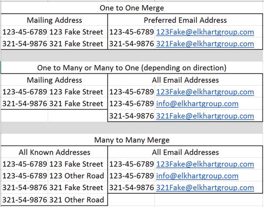
Figure 7-1. Some imaginary data showing how various merges might occur
It is worth noting that the difficulty with merging may well be in understanding what is being done rather than understanding the code itself. For data tables, the function call is merge(), and arguments control the type of merge that is performed. Due to the keyed nature of data tables, merging by the key choice can be quite efficient. Choosing to merge by nonkey columns is also possible, but will not be as efficient computationally.
Before getting into the first merge code example , we generate four data tables with information unique to each. All are keyed by Species from the iris data set. In real life, such code is not required because normally data tables come already separated. This code is included only for reproducibility of the merge results. Also note that these are very short data sets; the goal here is for them to be viewed and fully understood independently. This provides the best environment from which to understand the final merge results.
diris <- diris[, .(Sepal.Width = Sepal.Width[1:3]), keyby = Species]diris2 <- unique(diris)dalt1 <- data.table(Species = c("setosa", "setosa", "versicolor", "versicolor","virginica", "virginica", "other", "other"),Type = c("wide", "wide", "wide", "wide","narrow", "narrow", "moderate", "moderate"),MedPW = c(TRUE, FALSE, TRUE, FALSE, TRUE, FALSE, TRUE, FALSE))setkey(dalt1, Species)dalt2 <- unique(dalt1)[1:2]dirisSpecies Sepal.Width1: setosa 3.52: setosa 3.03: setosa 3.24: versicolor 3.25: versicolor 3.26: versicolor 3.17: virginica 3.38: virginica 2.79: virginica 3.0diris2Species Sepal.Width1: setosa 3.52: versicolor 3.23: virginica 3.3dalt1Species Type MedPW1: other moderate TRUE2: other moderate FALSE3: setosa wide TRUE4: setosa wide FALSE5: versicolor wide TRUE6: versicolor wide FALSE7: virginica narrow TRUE8: virginica narrow FALSEdalt2Species Type MedPW1: other moderate TRUE2: setosa wide TRUE
Note
Note A one-to-one merge requires two keyed data tables, with each row having a unique key:
merge(x = dataset1, y = dataset2). The merge exactly matches a row from one data table to the other, and the result includes all the columns (variables) from both data tables. Whether nonmatching keys are included is controlled by the all argument, which defaults to FALSE to include only matching keys, but may be set to TRUE to include nonmatching keys as well.
In a one-to-one merge, there is at most one row per key. In the case of diris2, there are three rows, and each has a unique species. Similarly, in dalt2, there are two rows, and each has a unique species. The only common key between these two data sets is setosa. A merge() call on this one-to-one data compares keys and by default creates a new data table that combines only those rows that have matching keys. In this case, merging yields a tiny data table with one row. The original two data tables are not changed in this operation. The call to merge() takes a minimum of two arguments; the first is x, and the second is y, which represent the two data sets to be merged.
merge(diris2, dalt2)Species Sepal.Width Type MedPW1: setosa 3.5 wide TRUE
Notice that what has been created is a complete data set. However, it is quite small, because the only results returned were those for which full and complete matches were possible. Depending on the situation, different results may be desired from a one-to-one merge. Perhaps all rows of diris2 are wanted regardless of whether they match dalt2. Conversely, the opposite may be the case, and all rows of dalt2 may be desired regardless of whether they match diris2. Finally, to get all possible data, it may be desirable to keep all rows that appear in either data set. These objectives may be accomplished by variations of the all = TRUE formal argument. In particular, note how to control which single data set is designated as essential to keep via the .x or .y suffix to all. If data is not available for a specific row or variable, the cell is filled with a missing value (NA).
merge(diris2, dalt2, all.x = TRUE)Species Sepal.Width Type MedPW1: setosa 3.5 wide TRUE2: versicolor 3.2 NA NA3: virginica 3.3 NA NAmerge(diris2, dalt2, all.y = TRUE)Species Sepal.Width Type MedPW1: other NA moderate TRUE2: setosa 3.5 wide TRUEmerge(diris2, dalt2, all = TRUE)Species Sepal.Width Type MedPW1: other NA moderate TRUE2: setosa 3.5 wide TRUE3: versicolor 3.2 NA NA4: virginica 3.3 NA NA
Note
A one-to-many or many-to-one merge involves one data table in which each row has a unique key and another data table in which multiple rows may share the same key. Rows from the data table with unique keys are repeated as needed to match the data table with repeated keys. In R, identical code is used as for a one-to-one merge: merge(x = dataset1, y = dataset2).
Merges involving diris and dalt2are of the one-to-many or many-to-one variety. Again, the behavior wanted in the returned results may be controlled when it comes to keeping only full matches or allowing various flavors of incomplete data to persist through the merge. The three examples provided are not exhaustive, yet they are representative of the different possibilities. The last two cases may not be desirable, as other has only one row, whereas most species have three.
merge(diris, dalt2)Species Sepal.Width Type MedPW1: setosa 3.5 wide TRUE2: setosa 3.0 wide TRUE3: setosa 3.2 wide TRUEmerge(diris, dalt2, all.y = TRUE)Species Sepal.Width Type MedPW1: other NA moderate TRUE2: setosa 3.5 wide TRUE3: setosa 3.0 wide TRUE4: setosa 3.2 wide TRUEmerge(diris, dalt2, all = TRUE)Species Sepal.Width Type MedPW1: other NA moderate TRUE2: setosa 3.5 wide TRUE3: setosa 3.0 wide TRUE4: setosa 3.2 wide TRUE5: versicolor 3.2 NA NA6: versicolor 3.2 NA NA7: versicolor 3.1 NA NA8: virginica 3.3 NA NA9: virginica 2.7 NA NA10: virginica 3.0 NA NA
So far, one-to-one and one-to-many merges have been demonstrated. These types of merges, or joins, have a final, merged number of rows that is at most the sum of the rows of the two data tables. As long as at least one of the dimensions of the merge are capped to one, there is no concern. However, in a many-to-many scenario, the upper limit of size becomes the product of the row count of the two data tables. In many research contexts, many-to-many merges are comparatively rare. Thus, the default behavior of a merge for data tables is to prevent such a result, and allow.cartesian = FALSE is the mechanism through which this is enforced as a formal argument of merge(). The same is not true for other data structures but is unique to data tables.
Attempting to merge diris and dalt1 results in errors from this default setting, which disallows merged table rows to be larger than the total sum of the rows. With three setosa keys in diris and two setosa keys in dalt1, a merged table would result with 3 x 2 = 6 total rows for setosa alone. As many-to-many merges involve a multiplication of the total number of rows, it is easy to end up with a very large database. Allowing this would yield the following results. Notice that this result has only complete rows.
merge(diris, dalt1, allow.cartesian = TRUE)Species Sepal.Width Type MedPW1: setosa 3.5 wide TRUE2: setosa 3.5 wide FALSE3: setosa 3.0 wide TRUE4: setosa 3.0 wide FALSE5: setosa 3.2 wide TRUE6: setosa 3.2 wide FALSE7: versicolor 3.2 wide TRUE8: versicolor 3.2 wide FALSE9: versicolor 3.2 wide TRUE10: versicolor 3.2 wide FALSE11: versicolor 3.1 wide TRUE12: versicolor 3.1 wide FALSE13: virginica 3.3 narrow TRUE14: virginica 3.3 narrow FALSE15: virginica 2.7 narrow TRUE16: virginica 2.7 narrow FALSE17: virginica 3.0 narrow TRUE18: virginica 3.0 narrow FALSE
The preceding has only complete rows and is missing the other species. Allowing all possible combinations nets two more rows, for a total of 20. It is an entirely different conversation if the resulting data is useful. When merging data, it always pays to consider what types of information are available, and what might be needed for a particular bit of analysis. We suppress rows 4 through 19 here:.
merge(diris, dalt1, all = TRUE, allow.cartesian = TRUE)Species Sepal.Width Type MedPW1: other NA moderate TRUE2: other NA moderate FALSE3: setosa 3.5 wide TRUE---20: virginica 3.0 narrow FALSE
For all of these, the key is Species, and that is only one column. Furthermore, it is nonunique. It is also possible to have keys based on multiple columns. Recognize that key choice may make all the difference between a one-to-one versus a many-to-many merge. Consider the following instructive example, in which only a single column is used as the key and the data is merged:
d2key1 <- data.table(ID1 = c(1, 1, 2, 2), ID2 = c(1, 2, 1, 2), X = letters[1:4])d2key2 <- data.table(ID1 = c(1, 1, 2, 2), ID2 = c(1, 2, 1, 2), Y = LETTERS[1:4])d2key1ID1 ID2 X1: 1 1 a2: 1 2 b3: 2 1 c4: 2 2 dd2key2ID1 ID2 Y1: 1 1 A2: 1 2 B3: 2 1 C4: 2 2 Dsetkey(d2key1, ID1)setkey(d2key2, ID1)merge(d2key1, d2key2)ID1 ID2.x X ID2.y Y1: 1 1 a 1 A2: 1 1 a 2 B3: 1 2 b 1 A4: 1 2 b 2 B5: 2 1 c 1 C6: 2 1 c 2 D7: 2 2 d 1 C8: 2 2 d 2 D
For the merge to be successful with its duplicated column names , ID2.x and ID2.y were created. The fact is, this data should have resulted in only four rows, once merged, because the data in those two columns is identical! By setting the key for both data sets to involve both columns ID1 and ID2, not only is the many-to-many merge reduced to a one-to-one merge, but the data is of a more practical nature. Multiple columns being used to key can be especially useful when merging multiple long data sets. For instance, with repeated measures on multiple people over time, there could be an ID column for participants and another time variable, but both would be used to merge properly. We discuss reshaping data next.
setkey(d2key1, ID1, ID2)setkey(d2key2, ID1, ID2)merge(d2key1, d2key2)ID1 ID2 X Y1: 1 1 a A2: 1 2 b B3: 2 1 c C4: 2 2 d D
Reshaping Data
In addition to being merged, data may be reshaped. Consider our iris data set: each row represents a unique flower measurement, yet many columns are used for each flower measured. This is an example of wide data. Despite not having a unique key, there are a variety of measurements for each flower (row). Wide data may be reshaped to long data, in which each key appears multiple times and stores variables in fewer columns. First, we reset our data to the iris data set and create a unique ID to be our key based on the row position. Recall that data tables suppress rows, so we add those into their ID column by using another useful shorthand of data tables, namely .N for number of rows:
diris <- as.data.table(iris)diris[, ID := 1:.N]setkey(diris, ID)dirisSepal.Length Sepal.Width Petal.Length Petal.Width Species ID1: 5.1 3.5 1.4 0.2 setosa 12: 4.9 3.0 1.4 0.2 setosa 23: 4.7 3.2 1.3 0.2 setosa 3---148: 6.5 3.0 5.2 2.0 virginica 148149: 6.2 3.4 5.4 2.3 virginica 149150: 5.9 3.0 5.1 1.8 virginica 150
Note
Reshaping is used to transform data from wide to long or from long to wide format. In wide format, a repeatedly measured variable has separate columns, with the column name indicating the assessment. In long format, a repeated variable has only one column, and a second column indicates the assessment or “time.” Wide-to-long reshaping is accomplished by using the melt() function, which requires several arguments.
To reshape long, we melt()the data table measure variables into a stacked format, which is based on the reshape2 and reshape packages (Wickham, 2007), although there is a data.table method for melt(), which is what is dispatched in this case. This function takes several arguments, which we’ll discuss in order. To see all the arguments, examine the help: ?melt.data.table. Note that it is important to specify the exact method, melt.data.table, because the arguments for the generic melt() function are different.
The first formal, data, is the name of the data table to be melted, followed by id.vars, which is where the ID variables and any other variable that should not be reshaped long. By default, id.vars is any column name not explicitly called out in the next formal. Any column name assigned to id.vars is not reshaped into long form; it is repeated, but left as is. The third formal is for the measure variables, and measure.vars uses these column names to stack the data. Typically, this is a list with separate character vectors to indicate which variables should be stacked together in the long data. The fourth formal is variable.name, which is the name of the new variable that will be created to indicate which level of the measure.vars a specific row in the new long data set belongs to. In the following example, the first level is for length measurements, while the second level corresponds to width measurements of iris flowers. Finally, value.name is the name of the molten (or long) column(s), which are the names of the columns in our long data containing the original wide variables’ values.
Describing reshaping and the required arguments is rather complex. It may be easier to compare output between the now familiar iris data set and the reshaped, long iris data set, shown here:
diris.long <- melt(diris, measure.vars =list( c("Sepal.Length", "Sepal.Width"), c("Petal.Length", "Petal.Width")),variable.name = "Type", value.name = c("Sepal", "Petal"),id.vars = c("ID", "Species"))diris.longID Species Type Sepal Petal1: 1 setosa 1 5.1 1.42: 2 setosa 1 4.9 1.43: 3 setosa 1 4.7 1.3---298: 148 virginica 2 3.0 2.0299: 149 virginica 2 3.4 2.3300: 150 virginica 2 3.0 1.8
Notice that our data now takes 300 rows because of being melted. The Type 1 versus 2 may be confusing to equate with length versus width measurements for sepals and petals. The melt() method for data tables defaults to just creating an integer value indicating whether it is the first, second, or third (and so forth) level. To make the labels more informative, we use factor(). Because factor will operate on a column and change the row elements of the column, it belongs in the second formal j argument of the data table.
diris.long[, Type := factor(Type, levels = 1:2, labels = c("Length", "Width"))]diris.longID Species Type Sepal Petal1: 1 setosa Length 5.1 1.42: 2 setosa Length 4.9 1.43: 3 setosa Length 4.7 1.3---298: 148 virginica Width 3.0 2.0299: 149 virginica Width 3.4 2.3300: 150 virginica Width 3.0 1.8
The data set diris.longis a good example of a long data set. It is not, however, the longest possible data set from diris—not that such a thing is necessarily a goal, by any means. However, should melt() be called on just diris along with calling out id.vars, the resulting data table is perhaps the longest possible form of the iris data. Just as id.vars defaults to any values not in measure.vars, so too measure.vars defaults to any values not in id.vars. As you can also see, variable.name and value.name default to variable and value, respectively. Notice that diris.long2 has 600 rows, and what were formerly the four columns of sepal and petal lengths and widths are now two columns. Also note that when this is done, melt() automatically sets the values of variable to the initial variable names from the data set.
diris.long2 <- melt(diris, id.vars = c("ID", "Species"))diris.long2ID Species variable value1: 1 setosa Sepal.Length 5.12: 2 setosa Sepal.Length 4.93: 3 setosa Sepal.Length 4.7---598: 148 virginica Petal.Width 2.0599: 149 virginica Petal.Width 2.3600: 150 virginica Petal.Width 1.8
Note
To reshape data from long to wide, the dcast() function is used. Two required arguments are data and formula, which indicate how the data should be reshaped from long to wide. The formula must indicate unique values in a cell, or the data needs to be aggregated within a cell.
While melt() is used to make wide data long, dcast() is used to make long data wide. Without unique identifiers for data, multiple values must be aggregated to fit in one cell. Thus, calling our casting function without some thought may create unwanted results (although sometimes aggregating multiple values is exactly what is desired). Notice that in the second formal, Species is called out as the identity key, and variable is named as the location to find our new column names:
dcast(diris.long2, Species ∼ variable)Aggregate function missing, defaulting to 'length'Species Sepal.Length Sepal.Width Petal.Length Petal.Width1: setosa 50 50 50 502: versicolor 50 50 50 503: virginica 50 50 50 50
If this long data is to be better cast to wide, a unique identifier is needed so that the formula creates unique cells that contain only one value. Unless aggregating results is desired, for a given variable, the formula argument should result in a single value, not multiple values.
In this case, since there are four possible values that the variable column takes on in the long data, as long as there is a unique key that is never duplicated over a specific variable such as Sepal.Length, the cast works out. In other words, if the wide data has a unique key, we can combine that unique key with the variable names in the long data, which together will exactly map cells from the long data set back to the wide data. The left side of the formula contains the key or ID variable. This side of the formula (left of the tilde, ∼) may also contain any other variable that does not vary (such as would have been specified using the id.vars argument to melt() if the data had initially been reshaped from wide to long). The right-hand side of the formula (after the tilde, ∼) contains the variable or variables that indicate which row of the long data set belongs in which column of the new wide data set.
In our long iris data set example, the ID and Speciesvariables do not vary and so belong on the left side. The variable called variable indicates whether a particular value in the long data set represents Sepal.Length, Sepal.Width, Petal.Length, or Petal.Width. Thus, for this example, the formula looks like ID + Species ∼ variable:
diris.wide2 <- dcast(diris.long2, ID + Species ∼ variable)diris.wide2ID Species Sepal.Length Sepal.Width Petal.Length Petal.Width1: 1 setosa 5.1 3.5 1.4 0.22: 2 setosa 4.9 3.0 1.4 0.23: 3 setosa 4.7 3.2 1.3 0.2---148: 148 virginica 6.5 3.0 5.2 2.0149: 149 virginica 6.2 3.4 5.4 2.3150: 150 virginica 5.9 3.0 5.1 1.8
Going back to the first diris.long data with the two-level factor for length and width of sepals and petals, it is also possible to cast this back to wide. The call to dcast() begins similarly to our previous example. We specify the long data set, a formula indicating the ID and Species variables that are not stacked, and the variable, Type, that indicates what each row of the data set belongs to.
In such not-so-long (for lack of a better word) data, we require an additional argument, the value.var formal, to let dcast() know which variables in the long data are repeated measures. This can be a character vector of every variable in the long data set that will correspond to multiple variables in the wide data set—in our case, Sepal and Petal, which in the long data contain both lengths and widths, as indicated in the Type variable. Additionally, the separator must be chosen, as data table column names may have different separators. This is selected via the sep = formal, and here we use the full stop for continuity’s sake, as that is how the variables were labeled in the original wide iris data set. We show merely the dcast() command, and check that regardless of method, the wide data is recovered via the all.equal() function, which checks for precisely what it states. To view the results, type diris.wide at the console:
diris.wide <- dcast(diris.long, ID + Species ∼ Type,value.var = list("Sepal", "Petal"), sep = ".")all.equal(diris.wide2, diris.wide)[1] TRUE
Summary
In this chapter, you met one of the two powerful (and more modern) ways of managing data in R. In particular, the type of data we manipulate with data.table is column and row, or table, data. In the next chapter, we delve more deeply into data manipulation. From there, you’ll meet dplyr, which is the other modern way of managing data in R. We will close out this section with a look at databases outside R. Table 7-1 provides a summary of key functions used in this chapter.
Table 7-1. Key Functions Described in This Chapter
Function | What It Does |
|---|---|
d[i, j, by] | General structure of a call to subset, compute in, or modify a data table. |
as.data.table() | Coerces a data structure to a data table. |
setkey() | Takes a data table in the first formal and then creates a key based on the column name arguments next passed to the function. |
haskey() | This function is called on a data table and returns a Boolean value. |
key() | Returns the data table’s key if it exists. |
order() | Controls the order to be ascending or descending for the data of a column. |
tables() | Returns any current data tables currently active. |
anyDuplicated() | Returns the location of the first duplicated entry. |
duplicated() | Returns TRUE or FALSE for all rows to show duplication. Can take a key. Otherwise, it is by all columns. |
unique() | Returns a data table that has only unique rows. Again, these may be specified to be specific rows. If there is a key, it is based on the key. If there is no key, it is based on all columns. |
setnames() | Allows column names to be changed. |
setcolorder() | Allows column order to be adjusted. |
:= | Assignment operator within a data table. |
.() | Shorthand for list(). |
.N | Shorthand for number of rows in a data table, or number of rows in a subset, such as when a compute operation is performed by a grouping variable. |
merge() | Merges two data tables based on matching key columns. |
melt() | Converts wide data to long data. |
dcast() | Converts long data to wide data. |