Version Control

Up until now, we have discussed relatively casual code development, some basic programming, functions, and classes. Developing new R packages is more complex, with many more files to manage. With this greater complexity, it is helpful to have an efficient system for backing up files and for going back to earlier versions. Version control systems provide an excellent way both to back up code and to roll back changes to a prior version (for example, if changes to implement a new feature break an old feature or introduce a bug). Various version control systems exist, but perhaps the most popular now is the open source Git originally developed to provide version control for the Linux kernel . Git can be used directly from the command line or through a graphical interface, of which there are several. Many people use GitHub ( https://github.com/ ), a service that uses Git and hosts repositories online, freely for public projects. GitHub also provides a graphical interface for Windows and Mac OS ( https://desktop.github.com/ ). However, if you do not want to learn or use Git or another version control system, feel free to ignore this section as well as any commands related only to version control throughout this chapter.

We use Git (and GitHub) for Windows in this chapter to provide version control for the example R package we develop. Specifically, this book uses the Windows GitHub desktop client v3.3.0. Git repositories can be used solely on a local computer, but using them with GitHub makes it easy to collaborate on packages, and share early package code with others.

Setting up a Git repository is possible from the command line, but perhaps the most intuitive way for new users to create a new Git repository is online, directly through GitHub. We make a new repository for the R package we develop in this chapter and call it AdvancedRPkg. The repository is initialized with a README file, which we’ll edit shortly. We can tell Git to ignore certain files or files with particular extensions by adding them to a file called .gitignore. Each file or extension is listed on its own line. We can edit it later, but for now, we just have GitHub create one. Figure 6-1 shows the steps to do this.

Figure 6-1. GitHub page for creating the AdvancedRPkg repository

If all works as planned, the results should look something like Figure 6-2. The repository is empty, except for the README and .gitignore files .

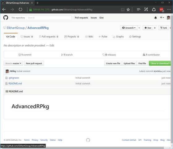
Figure 6-2. GitHub page showing the created AdvancedRPkg repository

From here, we can clone the repository to our local computer. Essentially, this creates a local copy, where we do our package writing. To do this, open the GitHub desktop client, click the + sign, select Clone, and then pick the repository, as shown in Figure 6-3.

Figure 6-3. GitHub desktop client cloning the AdvancedRPkg repository

After clicking Clone, we see an option to select a directory into which the repository should be cloned. Note that whatever directory you choose, a new directory is created for the repository with the same name as the repository (that is, AdvancedRPkg). Settings for the repository can be managed via the terminal, or by clicking the gear icon in the GitHub desktop client and choosing Repository Settings. One of them shows the currently ignored files. Files are ignored based on the .gitignore file , and because we selected R earlier when creating the repository, some default file extensions that are often desirable to ignore have been included by default (Figure 6-4).

Figure 6-4. GitHub desktop client showing settings for the AdvancedRPkg repository, including various file extensions that are ignored by the Git repository

Windows often creates temporary (sometimes hidden) files, desktop.ini, in directories. To avoid including these, we can edit the Repository settings by adding a new line at the end and typing desktop.ini. Then these files are ignored. Ignored files are those that the Git repository does not track and store changes in over time. They continue to exist in the directory; Git simply does not monitor and version them.

Aside from setting up a new Git repository, the tasks you are likely to do with Git are to commit changes to a repository and sync your local copy of the repository with the online (GitHub) version. Commits can be thought of as taking a snapshot of the state of files at the time of the commit. To avoid redundancy commits, snapshot only the changes made to files since the previous commit. Although even a slightly modified binary file may be difficult to compare, plain-text files, like R code, are easy to compare. Git is extremely efficient at tracking changes in text files over time and allowing you to either see what changes were made or go back to specific points in the past. Access to this history of a project (repository) is particularly helpful if errors or bugs are introduced into the code, so it can be pinpointed exactly when the bug was introduced (for example, how many results based on the code may be impacted?) and see previous working versions of code.

In slightly more complex use cases, Git can be effectively used to manage different versions of the code. For example, it is common to have a project and periodically release stable or production-ready versions of the code, while at the same time continuing development. This is accomplished in Git by using different branches of the same repository, and periodically merging some of the changes from one branch (say, the development branch) into the stable branch.

We show a few more relevant Git commands throughout this chapter. For more background on using Git, a great and free resource is Pro Git by Scott Chacon and Ben Straub (Apress, 2014), available at https://progit.org/ . For questions and answers, Stack Overflow ( http://stackoverflow.com ) is a good resource. It is likely someone else has already asked a question similar to yours, and if not, you can ask and get answers. Also note that if you use RStudio for your R code, it has some integration with Git built in. For more on this, see RStudio Support at https://support.rstudio.com/hc/en-us/articles/200532077-Version-Control-with-Git-and-SVN . Finally, note that you can access the online repository publicly at https://github.com/ElkhartGroup/AdvancedRPkg .

Starting a Package by Using DevTools

At a minimum, at the root directory of your package, you need DESCRIPTION and NAMESPACE files. You also need a subdirectory, R, which, sensibly, is where you put your R code. This is not enough for a package to submit to CRAN, but it is sufficient to start a functional package for private use. However, even for private use, proper documentation is incredibly helpful. The directory and file structure of packages is regrettably complex, especially to describe in text. Thus as a reference, the following is the final directory structure of our package that you should have by the end of this chapter, obtained from the within the AdvancedRPkg directory:

.
├── data
  │   └── sampleData.rda
├── DESCRIPTION
├── man
  │   ├── ggplot.lm.Rd
  │   ├── meanPlot.Rd
  │   ├── sampleData.Rd
  │   └── textplot-class.Rd
├── NAMESPACE
├── R
  │   ├── plot_functions.R
  │   ├── sampledata.R
  │   └── textplot.R
├── README.md
└── tests
    ├── testthat
      │   └── test_textplot.R
    └── testthat.R

5 directories, 13 files

For the initial setup, we use the function, setup(). We can specify more information, but the minimum is the path. We also set rstudio = FALSE so that the code works with any editor, not just RStudio. To see what has been created, we can use the list.files() function, which shows that DESCRIPTION and NAMESPACE files and an R directory have been created. For the following code, either run it from the R command line or make a new R file (we called ours chapter 06 .R). Note that it is important to adjust the path argument to point to the directory with the Git repository, wherever you cloned that on your local machine. In our case, R’s working directory (which you can check by calling the getwd() function) is in the directory directly above the AdvancedRPkg directory. If your R session is not there, either adjust the path argument or change R’s working directory to be in the parent directory to AdvancedRPkgby using the setwd() function:

setup(                  
  path = "AdvancedRPkg/",                  
  rstudio = FALSE)                  
Creating package 'AdvancedRPkg' in '∼/Apress_AdvancedR/RFiles'
No DESCRIPTION found. Creating with values:

Package: AdvancedRPkg
Title: What the Package Does (one line, title case)
Version: 0.0.0.9000
Authors@R: person("First", "Last", email = "[email protected]", role = c("aut", "cre"))
Description: What the package does (one paragraph).
Depends: R (>= 3.3.1)
License: What license is it under?
Encoding: UTF-8
LazyData: true

list.files("AdvancedRPkg")                  
[1] "DESCRIPTION" "NAMESPACE"   "R"           "README.md"  

The output also shows some of the fields and the information used to fill them in. Since most of these are placeholders, we want to open the files by using a text editor (any should be fine, including RStudio) and modify them. From the directory, setup() guesses the package name, but the rest need to be filled out. Using the editor, we change those fields to the following:

Package: AdvancedRPkg
Title: An Example R Package for the Book Advanced R
Version: 0.0.0.9000
Authors@R: c(
  person("Matt", "Wiley", email = "[email protected]", role = c("aut")),
  person("Joshua F.", "Wiley", email = "[email protected]", role = c("aut", "cre")),
  person("Elkhart Group Ltd.", role = "cph")
  )
Description: This package will demonstrate the basics of an R
  package including documentation and tests.
Depends: R (>= 3.3.1)
License: GPL (>= 3)
Encoding: UTF-8
LazyData: true

Note the version number, which is designed in the format Major.Minor.Patch.DevelopmentVersion. A good overview of the considerations in determining software versions is described at the Semantic Versioning specification at http://semver.org/ . It is quite prescriptive in its recommendations, but it is often helpful to have a fixed set of rules in place for determining a major or minor version of the software. The final piece, the DevelopmentVersion, is present only in development versions and is dropped for release. Despite these rules and guides, the reality of many R packages is far more heterogeneous and inconsistent (not everyone agrees on these rules, and even those who agree do not always strictly follow them).

Next up are the authors, described using the person() function. In addition to each individual’s name and e-mail, three-letter abbreviations are used to describe roles and relations. All possibilities are outlined in the MARC Code List for Relators at www.loc.gov/marc/relators/relaterm.html . However, the most commonly used ones are aut for the author, cre for a creator who is the person responsible for the project (or in R terms, the person to complain to if there are problems—the maintainer), and cph for the copyright holder. Then we provide a few sentences for a description of the package, specify the R version our package depends on, the license, and that data can be loaded on demand (saving startup time).

Adding R Code

With the basics of a package in place, it is time to start adding some R code, the whole point of a package! Since the focus of this chapter is on packaging the code, we reuse some functions and classes from previous chapters. As a first step, we create two files located in the AdvancedRPkg/R/ directory: plot_functions.R and textplot.R.

Next, we copy the final meanPlot() function from Chapter 4 to make a plot with means. We add the code for this function along with the S3 method, ggplot.lm(), that we wrote in Chapter 5 and put both in plot_functions.R. Then, we copy the classes and methods (show and subset, which is the bracket operator, [) for the textplot class from Chapter 5 into textplot.R. Because it is easy to copy the wrong code, we suggest copying and pasting the code from our GitHub repository ( https://github.com/ElkhartGroup/AdvancedRPkg ). If everything works, it should look like this:

list.files("AdvancedRPkg/R")                
[1] "plot_functions.R" "textplot.R"

As a side note, it can be difficult to decide how many separate files to have. It does not matter for R, but it does make a difference for development. It is not good to have all your code in one file, nor to split every function, class, and method into a separate file. If the result is not too long, we try to group related functions (such as plotting functions) and to group related classes and methods. As common sense, even if you can, do not give files the same names differentiated only by use of lowercase or uppercase letters; it is also generally a bad idea to use special characters or symbols in file names.

Now that we have a basic package template, we can load the functions by using the load_all() function from devtools. All we have to do is specify the path to the package. We can now see that some of our functions are available in the package namespace, which we do by using the ls() function and specifying where we want it to list available objects:

load_all("AdvancedRPkg")                
Loading AdvancedRPkg
ls(name = "package:AdvancedRPkg")                
[1] "ggplot.lm" "meanPlot"  "textplot"

In Chapter 4, we briefly discussed scoping. Scoping becomes more important to understand when writing packages. Package authors can write functions with the same names as functions in other packages. Although these functions do not overwrite each other, it can be confusing to be clear about which function you intend to call. This is where the package namespace can be helpful. The namespace controls which functions from other packages are imported (and therefore used by code from within that package), and which functions from a package are exported so that they are publicly available to users of the package. You can import specific functions from other packages, using the import feature. If you want many functions from another package, you may decide to make your package depend on that other package, in which case all public functions are available to your package. Another difference between importing and depending on another package is what happens when your package is loaded. If package B depends on package A when a user calls library(B), package B and package A are both loaded and attached. If package B imports from package A, when a user calls library(B), package B gets loaded and attached, and package A is loaded but not attached. Because package A is loaded, its functions are available to code within package B, but they are not exposed directly to the user because package A was not attached. Even when package A (or package B) are loaded and attached, only the exported functions are publicly available to users. This is beneficial, as it allows package developers to write and document functions that are for internal use only. If you do not need to export a function, it is a good idea not to. If two R packages export functions of the same name, and a user loads and attaches both packages, the function from whichever package is loaded later masks the earlier one. For a user, the only choice then is to either not load and attach one package, or to be explicit with the function calls, using the double colon operator, PkgA::foo(), PkgB::foo(). With thousands of R packages and even more functions, exporting only necessary functions helps avoid such conflicts and masking of names.

All of this is controlled via the NAMESPACE file of a package. Although we did not look at it, our package does have a NAMESPACE file , which was created when we ran setup(). However, the load_all() function is unique in that by default when it loads a package, it exports all objects. This is because during development, it is often convenient to be able to call all functions whether they are exported or not.

Tests

With functions and methods added to our new package and working in R, we can begin to think about quality control. It is great to write code that runs, but it is also crucial that the code does what is intended. Now, what is intended and expected are not always the same (that is where documentation plays a critical role, which we cover next). Still, even for the developer, tests ensure that what is written does what it is supposed to do.

Tests may be written at any stage of package development. If functions, names, and features are radically changing, perhaps it is too early to start writing many tests. However, even if a package is not done, if some functions are relatively stable, writing tests early can be helpful. Writing tests earlier rather than later is helpful because it is often easier to write a test immediately after writing a function, when its purpose and the way it works are still fresh in your memory. (If you do not know or have forgotten how a function works, it is hard to test it adequately!). It is also helpful because if later functions build on earlier functions, testing along the way can help ensure that problems are due to the newly written functions and not to some previous building block.

Benefits aside, the practicalities of writing tests are made easier by the testthat package. First, we need to create a new subdirectory in our package called tests, located at AdvancedRPkg/tests/. Next, we create a second subdirectory inside the first named testthat (that is,, AdvancedRPkg/tests/testthat/), into which we create R source files that run a variety of tests. Note there are other ways to test a package. Here we focus on doing so by using the testthat package paradigm.

It is rather difficult to test graphing functions properly, so for our tests, we check whether the subset method for textplot works as intended. We can make a file called test_textplot.Rlocated under AdvancedRPkg/tests/testthat/. We begin with a call to context(), which indicates that the tests that follow test related functionality, and we provide the overall name for a suite of tests, textplot. Next we set up a simple textplot class object, and then run a series of tests. The tests have two components. First, an outer call to test_that(). The first argument is a description of the test, and the second is code to do the tests. The code can consist of anything, but commonly includes calls to one of the expect_*() functions, of which there are many. We use the apropos() function call to show all the options for expect_*() before we make our choices:

apropos("expect_")                
 [1] "expect_cpp_tests_pass"     "expect_equal"             
 [3] "expect_equal_to_reference" "expect_equivalent"        
 [5] "expect_error"              "expect_failure"           
 [7] "expect_false"              "expect_gt"                
 [9] "expect_gte"                "expect_identical"         
[11] "expect_is"                 "expect_length"            
[13] "expect_less_than"          "expect_lt"                
[15] "expect_lte"                "expect_match"             
[17] "expect_message"            "expect_more_than"         
[19] "expect_named"              "expect_null"              
[21] "expect_output"             "expect_output_file"       
[23] "expect_s3_class"           "expect_s4_class"          
[25] "expect_silent"             "expect_success"           
[27] "expect_that"               "expect_true"              
[29] "expect_type"               "expect_warning"           

We choose expect_is() to check the class of the object and expect_equal() to check other features. It is also possible to check that your error checking is working, using expect_error() or expect_warning(), which “pass” if the code creates an error. We place the following code into our test_textplot.R file:

context("textplot")                  

dat <- textplot(                  
  x = 1:4,                  
  y = c(1, 3, 5, 2),                  
  labels = letters[1:4])                  

test_that("textplot subset method works with rows only", {                  
  tmp <- dat[i = 1:2, ]                  
  expect_is(tmp, "textplot")                  
  expect_equal(length(tmp@x), 2)                  
})                  

test_that("textplot subset method works with variables only", {                  
  tmp <- dat[, j = c("x", "y")]                  
  expect_is(tmp, "list")                  
  expect_equal(length(tmp), 2)                  
  expect_equal(length(tmp$x), 4)                  
})                  

test_that("textplot subset method works with rows and variables", {                  
  tmp <- dat[1:2, j = c("x", "y")]                  
  expect_is(tmp, "list")                  
  expect_equal(length(tmp), 2)                  
  expect_equal(length(tmp$x), 2)                  
})                  

We can run the code tests directly. If everything works, there is no output. Output is created only when something does not pass the checks. However, typically, this code is not run directly; it is run in batches. We run all tests by using the devtools function, test(), and our package name/path. The devtools package knows the directory structure for the testthat package, and so they play nicely together. To run the tests, test() first loads the package by using load_all() and then executes the tests. Back in the folder above the package directory, from our chapter-level R file, chapter06.R, we run all the tests by executing the code that follows:

test("AdvancedRPkg")                  
Loading AdvancedRPkg
Testing AdvancedRPkg
textplot: ........

DONE =================================================================

Errors would be noted, if present. Although we can run the tests as is by using the devtools package, for R to run them, we need to add a short file in the tests directory (that is, AdvancedRPkg/tests/), called testthat.R. Into this file, we just need to add a few lines of code, shown next. We do not run this code; this is run by R:

library(testthat)                  
library(AdvancedRPkg)                  

test_check("AdvancedRPkg")                  

Now, we can use the covr package to check code coverage. The covr package ( https://github.com/jimhester/covr ) checks whether different parts of the code are run when a test is executed. For example, a function that contains if/else statements may have only part of its code executed by one test, unless additional tests are derived to check the other conditions. Again, although not required to develop a package, it is a helpful tool to see how well the current tests cover the package functionality. A high level of coverage (aiming toward 100 percent) is a good way to catch bugs and to ensure that new code development does not break old features and functionality; and all of this can also help to assure users that your package is a good choice.

While we used the checkpoint library to allow code reproducibility, the nature of testing precludes such library usage from being effective. Thus, installing both covr and testthat is required. Back in our top-level chapter06.R file, we run the package_coverage() function to test how well our tests cover our small package’s code. The only argument required is the directory where the package is located. In our case, R’s working directory is the parent directory, AdvancedRPkg/. If the working directory for your R instance is different, you need to specify the appropriate path to get to the AdvancedRPkg/ directory on your machine:

install.packages(c("covr", "testthat"))                
cov <- package_coverage("AdvancedRPkg")                

The output (shown next) indicates that current testing coverage is about 36 percent, and this is driven by coverage of code from textplot.R. It is also possible to get a more detailed analysis, using as.data.frame(cov). The output is substantial, so we show just a few rows and columns, but it is an invaluable resource if you think you have tests covering everything and need to figure out what aspects of your code are not being tested yet:

cov                  
AdvancedRPkg Coverage: 35.85%
R/plot_functions.R: 0.00%
R/textplot.R: 52.78%

as.data.frame(cov)[1:3, c(1, 2, 3, 11)]                  
            filename functions first_line value
1 R/plot_functions.R  meanPlot          2     0
2 R/plot_functions.R  meanPlot          3     0
3 R/plot_functions.R  meanPlot          4     0

To have the tests run, we need to indicate that our package requires the testthat package. The core functionality of the package does not depend on testthat, so instead we add it to the DESCRIPTION file under a new section, Suggests. Again, using any text editor, we revise DESCRIPTION to the following:

Package: AdvancedRPkgPackagetests
Title: An Example R Package for the Book Advanced R
Version: 0.0.0.9000
Authors@R: c(
  person("Matt", "Wiley", email = "[email protected]", role = c("aut")),
  person("Joshua F.", "Wiley", email = "[email protected]", role = c("aut", "cre")),
  person("Elkhart Group Ltd.", role = "cph")
  )
Description: This package will demonstrate the basics of an R
  package including documentation and tests.
Depends: R (>= 3.3.1)
Suggests:                
  testthat                
License: GPL (>= 3)
Encoding: UTF-8
LazyData: true

Finally, with all the changes we have made to our package, it is time to check in with version control. It is possible to do this from the command line, but we use the GitHub desktop client. By default, all changed files are selected, but rather than commit all changes at once, we do them in related batches of files, along with meaningful messages. The commit messages are added along with each commit and serve to remind you or to let others know a high-level summary of what changes were made or why. It is not necessary to detail every change, as Git takes care of tracking exactly which files changed and how their contents changed.

To begin, we select the DESCRIPTION, NAMESPACE, and .gitignore files and add the message: initiate R package with DESCRIPTION and NAMESPACE. The process is shown in Figure 6-5.

Figure 6-5. GitHub desktop client selecting changed files, adding a commit message, and committing to the master branch

Next, we add plot_functions.R and textplot.Rand add the commit message: initial commit of R functions. Finally, we add testthat.R and test_textplot.R and add the commit message: adding testing for quality control. Of course, you also could have committed files along the way as they were created. If we switch over to the History tab of the GitHub desktop client, we can see the changes made. If we are happy for them to go public, we click the Sync button, which pulls changes from the GitHub repository to the local repository, and pushes all committed changes from the local repository to the GitHub repository. Note that before you sync, all changes should be committed, because what gets synced are not the actual files in the directory but the Git repositories. Changes to files get added to the local Git repository only when they are committed, so if you do not commit, the updates are not added to the local repository and so do not get pushed to the remote (GitHub) repository. Figure 6-6 shows what this looks like.

Figure 6-6. GitHub desktop client showing the history of commits and the Sync button at the top right

We have only scratched the surface of testing , and obviously our package has a long way to go before it is thoroughly tested. However, these tools should get you started on the right track (and ahead of the majority of the R packages on CRAN) regarding testing and quality control. The next crucial piece is the documentation, a topic we turn to next.

Functions

To document objects using roxygen2, documentation is added after a special comment lead: ##' or #'. Because # is R’s comment, R ignores it, but the special single quote indicates to roxygen2 that this information should be processed into the documentation. Note that this syntax precludes commenting this code. All of this code is added to plot_functions.R above the meanPlot() function code.

As stated, comments are precluded because of syntax; thus the order becomes vital. To see which part maps to which formal, just keep in mind that there are three sections simply separated by line breaks: title, description, and details. The details section is optional. We add spaces between line breaks for reader clarity. Function arguments are indicated by using @param argument_name brief description of the argument. The argument names listed here must exactly match the named arguments in the function. The @return section is where we can indicate what sort of object is returned by the function. In this case, the function is called for the side effect of producing a plot, and the value it returns is not important. Any text can come after @author to indicate who wrote the function. Typically, the @author section is not required if the author is the same as the overall package author. For the function to be publicly available, it must be exported. This is accomplished by using the directive @export. The roxygen2 package translates this into additional lines of code in the NAMESPACE file, indicating it should be exported. The @keywords section is optional. Finally, one of the most useful sections for your readers is the @examples section, which gives readers executable examples and is one of the easiest ways to show how to use a function.

##' Function to plot data and mean summary
##'

##' This is a simple function designed to facilitate plotting raw
##' data along with dots indicating the mean at each x-axis value.
##'

##' Although this function can be used with any type of data that works
##' with code{plot}, it works best when the x-axis values are discrete,
##' so that there are several y-values at the same x-axis value so that
##' the mean of multiple values is taken.
##'

##' @param formula A formula specifying the variable to be used on the
##'   y-axis and the variable to be used on the x-axis.
##' @param d A data.frame class object containing the variables specified
##'   in the code{formula}.

##' @return Called for the side effect of creating a plot.
##' @author Wiley
##' @export
##' @keywords plot
##' @examples
##' # example usage of meanPlot
##' meanPlot(mpg ∼ factor(cyl), d = mtcars)

Now to make the documentation, we can run the roxygen2 package. This can be done directly by using the roxygenize() function and giving it the path to the directory of our package, or it can be done by using the document() function from the devtools package. We specify the package directory, and the rest happens automatically. The output shows that a documentation file was written (meanPlot.Rd) and the NAMESPACE file was written:

document("AdvancedRPkg")                
Updating AdvancedRPkg documentation
Loading AdvancedRPkg
Updating roxygen version in  ∼RFilesAdvancedRPkg/DESCRIPTION
Writing NAMESPACE
Writing meanPlot.Rd

When built or installed, the R documentation file is converted to HTML and PDF. However, already you can preview the development version of the documentation. From the R console, the usual way of getting help for a function should now work:

?meanPlot                

If you use RStudio, you can also open the file and preview it. The resulting HTML file (after building the package) is shown in Figure 6-7. Because of the simplicity of this function and also for the sake of space, we wrote fairly minimal documentation. Often, it is helpful for users and future reference to document more extensively and to carefully explain what each argument can and cannot take. If functions implement new procedures or statistical methods, it is also common to include some references by using the @referencessection.

Figure 6-7. HTML output of the R documentation file for the meanPlot() function

Data

Before we can document data, we need to add some to our package. First, we make a data subdirectory in our package folder, located at AdvancedRPkg/data/. Then we make a small sample data frame and save it as an .rda file by using the code that follows in our chapter06.R file. Note again that the file needs to give the correct path to AdvacedRPkg/data/ based on R’s current working directory:

sampleData <- data.frame(                
  Num = 1:10,                
  Letter = LETTERS[1:10])                
save(sampleData, file = "AdvancedRPkg/data/sampleData.rda")                

We add the following code to document the data in a new file called sampledata.R located in the R subdirectory (that is, AdvancedRPkg/R/sampledata.R). This provides a title and details on the data, along with the special parameters @format to indicate the format or type of data and @source to indicate where it is from. In quotes at the end, the name of the object is given.

##' Numbers and letters.                
##'                
##' A sample data set containing 10 numbers and letters with two variables:                
##'                
##' itemize{                
##'   item Num. A number.                
##'   item Letter. An upper case letter (A to J)                
##' }                
##'                
##' @format A data frame with 10 rows and 2 variables                
##' @source Created as a sample                
"sampleData"                

After re-roxygenizing the package by using the document() function, the resulting HTML is shown in Figure 6-8, again by using the help utilities from the fully built package or by using preview from RStudio.

Figure 6-8. HTML output of the R documentation file for the sampleData data set

Classes

S3 classes are not formal and are not typically documented. S4 classes are straightforward to document. Their documentation goes immediately above the call to setClass() in our textplot.R file (AdvancedRPkg/R/textplot.R) with a title, a details section, and then some parameters— one @slot for each slot name, detailing the name and function of the slot. To use the S4 system in a package, we also need to add the methods package, which we do by adding @import methods and also adding it to the Imports field of the DESCRIPTION file. The updated DESCRIPTION file with the new Imports field is shown here; typically, the Imports section immediately follows the Depends section:

Imports:                
  methods                

The full documentation for the class is shown in the following code:

##' An S4 class to hold text and Cartesian coordinates for plotting                
##'                
##' A class designed to hold the data required to create a textplot                
##' where character strings are plotted based on x and y coordinates.                
##'                
##' @slot x A numeric value with the x axis coordinates.                
##' @slot y A numeric value with the y axis coordinates.                
##' @slot labels A character string with the text to be plotted                
##' @import methods                

After re-roxygenizing the package by using the document() function, the resulting HTML is shown in Figure 6-9.

Figure 6-9. HTML output of the R documentation file for the S4 class textplot

Methods

Documenting methods is similar to documenting regular functions. S3 methods can be undocumented or documented as a function. The following is the roxygen2-style documentation added for the ggplot.lm method. The code is added immediately above the function definition in AdvancedRPkg/R/plot_functions.R. Note that here we import the ggplot2 package so that it is available. We also add the ggplot2 package under the Imports section in the DESCRIPTION file, separated by a comma from the R version on which the package depends. The new DESCRIPTION file Depends section is shown here:

Imports:                
  methods,                
  ggplot2                

By importing it, roxygen2 will automatically add the appropriate import codes to the NAMESPACE file:

##' Method for plotting linear models                
##'                
##' Simple method to plot a linear model using ggplot                
##' along with 95% confidence intervals.                
##'                
##' @param data The linear model object from code{lm}                
##' @param mapping Regular mapping, see code{ggplot} and code{aes} for details.                
##' @param vars A list of variable values used for prediction.                
##' @param ldots Additional arguments passed to code{ggplot}                
##' @return A ggplot class object.                
##' @export                
##' @import ggplot2                
##' @examples                
##' ggplot(                
##'   lm(mpg ∼ hp * qsec, data = mtcars),                
##'   aes(hp, mpg, linetype = factor(qsec)),                
##'   vars = list(                
##'     hp = min(mtcars$hp):max(mtcars$hp),                
##'     qsec = round(mean(mtcars$qsec) + c(-1, 1) * sd(mtcars$qsec)), 1)) +                
##'   geom_ribbon(aes(ymin = LL, ymax = UL), alpha = .2) +                
##'   geom_line() +                
##'   theme_bw()                

S4 methods can be documented alone, documented with the generic function, or documented with the class. This can be accomplished by using the @describeIn parameter, which is used in place of the title. For our S4 methods, we document them along with the class. The roxygen2 code is relatively brief. We could add details but do not need to. The roxygen2 package takes care of registering the methods, so all we really need to do is add any special notes and document use of parameters. The documentation for the show() method is as follows:

##' @describeIn textplot show method                
##'                
##' @param object The object to be shown                

We follow this with the documentation for the [ operator method. Note that we also export the [ method and add an alias, which is just another way that users can look up the method:

##' @describeIn textplot extract method                
##'                
##' @param x the object to subset                
##' @param i the rows to subset (optional)                
##' @param j the columns to subset (optional)                
##' @param drop should be missing                
##' @export                
##' @aliases [,textplot-method                

After re-roxygenizing by using document(), the updated HTML help file is shown in Figure 6-10, including the class and additional methods documentation.

Figure 6-10. HTML output of the R documentation file for the S4 class textplot with added methods documentation