Search in book...
Toggle Font Controls
Create new playlist

Name your new playlist

Playlist description (optional)
Sign In

Email address

Password

Forgot Password?

or

Continue with Facebook

Continue with Google
Sign Up

Full Name

Email address

Confirm Email Address

Password

or

Continue with Facebook

Continue with Google

21
Quantifying the Variability of Wind Energy

Simon Watson

Centre for Renewable Energy Systems Technology, School of Electronic, Electrical and Systems Engineering, Loughborough University, Loughborough, LE67 5AH, UK

Wind by its very nature is a variable element. Its variation is different on different timescales and spatially its magnitude can change dramatically depending on local climatology and terrain. This has implications in a variety of sectors, not least in the wind energy sector. The accuracy of weather forecasting models has increased significantly in the last few decades, and these models are able to give insight into variability on the hourly and daily timescales. On shorter timescales, predicting chaotic turbulent fluctuations is far more challenging. Similarly, the ability to make seasonal forecasts is extremely limited. General circulation models (GCMs) can give insight into possible future decadal fluctuations, but there are still large uncertainties. Observational data can give useful information concerning variation on a variety of timescales, but data quality and spatial coverage can vary. An understanding of local scale spatial variations in wind is extremely important in wind farm siting. In the last 40 years, there have been significant advances in predicting these variations using computer models, although there remain significant challenges in understanding the behavior of the wind in certain environments. Both the spatial and temporal variations of wind are important considerations when wind power is integrated into electricity networks, and this will become an ever more important consideration as wind generation makes an increasing contribution to our global energy needs.

THE IMPORTANCE OF WIND VARIABILITY

Understanding how wind varies on both the temporal and spatial scales is important in many branches of the physical sciences and in engineering. Wind power is still a rapidly growing source of electricity generation, despite global economic uncertainties^[1], and understanding how it varies on these scales is extremely important for the energy industry. The advent of ever‐more‐powerful computers has allowed predictions of wind speeds in areas where measurements are sparse and has also provided an opportunity to try and predict future trends.

On a temporal scale, understanding the variation of wind speeds is important for the following:

Turbine design and siting on the very shortest timescales: ∼1 second
Operation of a power network on intermediate timescales: ∼1 hour to a few days
Energy yield on longer timescales: about months to years

An overview is given of our understanding of these latter two issues, using a variety of data sources and analysis methods.

Understanding the distribution of wind speeds at a site is important in terms of estimating the capacity factor and energy yield of a wind turbine, and a review of this is given to show how well the commonly used theoretical distributions fit observations. Longer‐term temporal and spatial variability will be addressed looking at research using observed surface data, proxy data such as pressure fields, and model data. Looking to the future, an overview of climate change‐related predictions of wind speeds is given for different regions.

Finally, an overview is given of the research to address the impact of wind variability on wind power generation. This will consider how geographical dispersion and wide area interconnection could help reduce overall variability and help the long‐term integration of wind energy into power systems.

AN OVERVIEW OF DIFFERENT SCALES OF VARIABILITY

Much of our understanding of the temporal variability of wind stems from work done by Van der Hoven^[2], despite shortcomings in the collection and analysis of the data underpinning this work. Figure 21.1 shows the power spectral density determined from wind speed data collected at the Brookhaven National Laboratory in the United States, which was the basis of Van der Hoven's work and which has been widely referenced since. It can be seen that the spectrum apparently shows three obvious peaks: one at around four days corresponding to the passage of weather systems; one at 12 hours reflecting a harmonic of the diurnal cycle; and one around one minute corresponding to turbulence. The reason for the lack of a 24‐hour peak is unclear and was put down to the measurements being made at around 100 minutes, although this does not explain why there was a 12‐hour peak. Between the 12‐hour peak and the turbulence peak, the magnitude of the spectrum drops to almost zero, and this has become known as the “mesoscale” or “spectral gap” and is often used as a justification for averaging wind speeds, for the purposes of climatological assessment, over 10‐minutes or 1‐hour intervals. However, the spectrum was derived from the data collected from more than one height over different periods, and in particular, the turbulent peak was determined purposely from the data collected over a day when a hurricane passed over the site. This was presumably to highlight the turbulence peak, as shown in Figure 21.1. Figure 21.2 shows a similar power spectral derived for one‐minute and five‐second data collected from the Science and Technology Facilities Council's Rutherford Appleton Laboratory (STFC‐RAL) site over a number of years (Barton; private communication). In contrast to the Van der Hoven spectrum, the turbulence peak is far less marked, and although there is evidence for a spectral gap there is still significant power in the spectrum at around one hour. There has since been much debate about the existence or otherwise of a spectral gap^[3–5], which, at the very least, suggests that it may well be site‐dependent. A strong diurnal cycle of wind speeds can be seen with a definite harmonic at 12 hours and evidence of a higher‐order harmonic at 6 hours (owing to an imperfect sinusoidal variation in daily wind speeds). There is a broad peak centered around 4 days although this would seem to be broader than in the case of the Van der Hoven spectrum. An annual cycle is obvious and there is evidence for some power in the spectrum at even longer timescales. Indeed, the longer term variability of wind speeds has been the subject of interest in recent years, particularly within the wind energy industry as developers and operators of wind farms try to determine expected long‐term energy yields, something which is of paramount importance for the financing of a particular installation. The evidence of variance at longer timescales is discussed below. It may be that variance on timescales longer than 50 years exists, but the data to infer this are scarce. The best that can be said is that variance can be expected at all scales, and that this leads to a degree of uncertainty in estimation of mean and turbulent quantities.

2 Power spectral density (m2/s2) vs. time scale (h) displaying a solid curve. — **Figure 21.1** The Van der Hoven spectrum of wind speeds at Brookhaven National Laboratory, USA.

Graph illustrating power spectrum density of wind speeds based on data collected at STFC‐RAL, UK displaying a fluctuating curve. — **Figure 21.2** Power spectrum density of wind speeds based on data collected at STFC‐RAL, UK.

A number of authors have commented on the lack of stationarity in wind speeds at various timescales^[5–7], and this presents a particular challenge when attempting to parameterize quantities such as mean wind speeds, turbulent time, and length scales, etc. Figures 21.1 and 21.2 lend support to this hypothesis, where it is seen that there is variance over a large range of timescales. What these figures cannot show is the degree of nonlinear interaction between the different scales of variation which surely exist. The separation of different scales of variability represents a significant challenge in many areas of wind engineering.

WIND SPEED DISTRIBUTIONS

The distribution of wind speeds at a site is important in terms of the expected capacity factor of a wind turbine. Commonly used is the so‐called Weibull distribution^[8], where the two‐parameter form of the probability density function f is given by

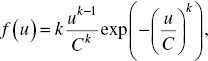
when observing a wind speed u with Weibull scale, C and shape, k parameters. This has been shown to fit well at many sites^{[9, 10]} and can be used to provide an accurate estimate of wind energy production^[11]. However, discrepancies have been noted, e.g. in the United States where this distribution fits wind speeds well during the day, but at night, wind speeds are observed to be more positively skewed^{[12, 13]}. From scatterometer data, offshore wind speeds have been shown to be almost Weibull distributed, but the skewness of the observed distribution was found to be more strongly negative in the Tropics, and more strongly positive in Northern Hemisphere mid‐latitudes, than would be expected for a true Weibull distribution^[14]. This behavior was found to be consistent for all seasons^[15]. Scatterometer data from extra‐tropical latitudes were seen to not follow a Weibull distribution, although this was partly attributed to data cutoff below 2 m s⁻¹^[16]. Scatterometer data off the coast of Japan were compared with buoy data showing good agreement with these data and were well‐fitted by a Weibull distribution^[17]. A study of scatterometer‐derived wind speeds in the North and Baltic Seas^[18] showed a relatively small bias in mean wind speed compared with observations, although problems in the interpretation and processing of scatterometer data are acknowledged owing to the effects of rain, atmospheric stability, varying sea surface temperature, oceanic currents, and proximity to land. On the other hand, wind speed data from sites in the North Sea measured on platforms have been shown to be well fitted by a Weibull distribution^[19].

Where wind speed distributions are bimodal, or where a large number of calms or low wind speeds are observed^[20], a single Weibull distribution may not be appropriate^[21], although poor‐quality anemometry at low speeds may be partly responsible^[22]. In such cases, a combination of two Weibull distributions has been found to provide a better fit^[21–24]. An example of three different functions fitted to an observed distribution of wind speeds is shown in Figure 21.3 ^[25]. It can be seen that the combination of the two Weibull probability density functions is able to capture the bimodal nature of this wind speed distribution with the singly truncated from below normal Weibull (TNW) probability density function better capturing the large number of calms.

Image described by caption and surrounding text. — **Figure 21.3** Histogram of observed wind speeds with three theoretical distributions fitted. W, Weibull; WW, bi‐modal Weibull; TNW, singly truncated from below normal Weibull.
Source: Reprinted with permission from Ref.^[25]. Copyright 2007 Elsevier.

LONG‐TERM TRENDS

A View from Observations

The most obvious way to assess long‐term variability of wind speeds is to examine historic long‐term records of surface station observations. A map summarizing the results of 148 studies^[26] is shown in Figure 21.4. What is striking is the overall trend of reducing wind speeds. When the authors averaged all studies, this led to an average global change in wind speeds of −0.014 m s⁻¹ per year. In a similar study^[27], a trend of declining worldwide wind speeds was seen, although it was noted that the statistical relevance of some of the trends was hard to assess. Another study of global long‐term wind speeds suggested that over the Northern Hemisphere, wind speeds have declined −0.011 m s⁻¹ per year over a period of 30 years^[28]. There may be a number of reasons for this, but another significant observation, also noted in Ref.^[5], is an apparent trend to increasing wind speeds at exposed coastal sites. This leads to a possible explanation of increasing surface roughness on land due to vegetation cover or due to urbanization.

Shaded world map illustrating the trends in observed surface wind speeds (in m/s per annum) with discrete shaded areas corresponding to the scale bar of u trend (m/s/a) on the right. — **Figure 21.4** Trends in observed surface wind speeds (in m/s per annum).
Source: Reprinted with permission from Ref.^[26]. Copyright 2012 Elsevier.

No data are shown for the United Kingdom, but two recent studies have been made of wind speeds in this region. On the basis of ∼50 years of data^[29], it was observed that winds over the United Kingdom as a whole did not seem to show a significant change once historic changes to measurement height were taken into consideration; however, there was a tentative tendency to lower wind speeds in the northwest of the United Kingdom and greater wind speeds in the southeast. Over the central belt of Scotland, there was evidence for reduced wind speeds over a ∼40‐year period^[30].

It is clear from the above studies that it is difficult to distinguish wind speed changes that are climatologically driven from those resulting from other site‐specific factors. The use of surface wind speed observations is problematic where the quality of the data is unknown, with regard to factors such as anemometer type and calibration, siting, exposure, and measurement height. It is also difficult to draw definitive conclusions from datasets covering different time periods and where observations are sparse.

Some researchers have turned to the use of pressure measurements to try and overcome this problem^[31–33]. For example, pressure triangles based on site measurements of atmospheric pressure were used to infer a pressure gradient and therefore the geostrophic wind^[33] for the period 1984–2007 for the northeastern Atlantic region. In a similar, much earlier study^[34], a gridded dataset of pressure measurements was used to derive pressure gradients and a set of linear regression equations developed to predict long‐term monthly wind speed records at a number of UK sites for the period 1881–1989. The North‐Atlantic Oscillation (NAO) index has long been known to correlate to observed wind speeds in northern Europe, particularly during winter. This index is traditionally based on the pressure difference between a site in Iceland and the Azores. Using this index, it has been shown^[35] that there is up to a 10% difference in wind power predicted output between high and low NAO states, implying a significant degree of interannual variability.

Several proxies for surface wind speed have been studied including the NAO, as well as the Grosswetterlagen, and Jenkinson Lamb indices^[36], the latter two being popular weather system classification schemes. These showed a reasonable degree of agreement (R² = 0.49) and suggested a downward trend in windiness across northwestern Europe in the 15‐year period 1990–2005, although there was an upward blip during the 1990s. It could also be seen that over the longer term (1965–2005), this downward trend was not apparent. The conclusion from this work was that care should be taken when choosing an appropriate historic period to assess the expected long‐term wind‐speed climate at a prospective wind farm site.

A View from Model Data

More recently, researchers have turned to numerical models to produce more consistent datasets in order to analyze long‐term geographical trends in wind speeds. One particular form of numerical model output that has been used for this purpose is referred to as reanalysis. Reanalysis datasets are produced by assimilating a large number of different meteorological datasets including: satellite measurements, ship‐borne and buoy observations, land‐based surface observations, upper air measurements, and remote sensing observations. The data are input to a general circulation model (GCM), which is essentially a numerical weather prediction model that can be used to produce “hindcast” values of a range of meteorological variables on a regular grid at discrete time intervals. Such output data are effectively homogenized and avoid some of the problems associated with local effects, which are seen at specific surface stations. For that reason, reanalysis data are suitable for constructing long‐term regional climatologies. Two notable examples include the National Centers for Environmental Prediction (NCEP)/National Center for Atmospheric Research (NCAR)^[37] and the European Centre for Medium‐Range Weather Forecasts (ECMWF) ERA‐40^[38] reanalysis datasets. These and other similar datasets have been used to study long‐term wind speed trends in several parts of the world.

Europe

An analysis of 850‐mb winds from NCEP/NCAR reanalysis data^[39] suggests a general increase in wind speeds over the Baltic region with the majority of the increase during the winter. Over higher altitudes in Switzerland there is evidence for reducing wind speeds with the decline observed to be more rapid than at lower altitudes^[40]. A note of caution is sounded in using reanalysis datasets to infer wind speed statistics at sites. It has been seen that when comparing reanalysis wind speed distributions with observations in Hungary^[41], there are differences in the shape of these distributions and care needs to be taken when rescaling 10 m values to typical wind turbine hub height.

United States

The Modern‐Era Retrospective Analysis for Research and Applications (MERRA) reanalysis dataset^[42] was studied to consider spatial variation in wind speed and potential wind power trends across the United States^[43]. The wind power density (WPD) and variability or robust coefficient of variation (RCoV) were determined, showing large variation across the country. The RCoV is defined as

The RCoV gives a better measure of variability when a distribution is non‐Gaussian distributed. Figure 21.5 shows the geographical variation in RCoV across the United States, including off the East and West Coasts. There are clear differences in trends between the eastern and western sides of the United States, as well as in the offshore regions, which have implications for wind energy variability.

A comparison was made between wind speed trends from two observational datasets, four reanalysis datasets, and two regional climate models (RCMs) in the United States^[44]. This showed conflicting results with the observed data indicating a significant long‐term decline in wind speed over time. The model data results differ, with one reanalysis dataset and one of the RCMs indicating a decline, but the other models showing an increase.

The North American Regional Climate Change Assessment Program (NARCCAP) uses a combination of a GCM and an RCM to produce high‐resolution datasets on a regular grid^[44]. This was used to study trends in wind speeds over the western High Plains for the period 1971–2000^[45]. A significant decline in wind speeds was seen in all seasons (up to 20%) with the exception of autumn (fall) season where an increase of up to 10% was seen. This study extrapolated wind speeds from 10 to 80 m above the ground using the 1/7 power law. In another study, the North American Regional Reanalysis Dataset (NARR)^[46] was used to estimate 80‐m wind speeds by interpolating between the closest model levels^[47]. By contrast, this study found increasing wind speeds for the period 1979–2009. This was put down to the strengthening of low‐level jets, which are not as apparent at lower altitudes. The findings of this study were consistent with those of an earlier study looking at changes in wind speeds over the Great Lakes region of the United States^[48].

FUTURE TRENDS

Atmosphere–ocean general circulation models (AOGCMs) can be used to make climate projections into the future. By including future carbon dioxide emissions in a model run according to various emission scenarios as defined by the Intergovernmental Panel on Climate Change (IPCC)^[49], changes in world climate can be determined. This has been done using a number of well‐known AOGCMs such as HadCM3, ECHAM5, and (Parallel Climate Model) PCM. The IPCC issues periodic Assessment Reports (ARs), including details of the results of these models, e.g. Ref.^[50]. Downscaling of the AOGCM data using RCMs allows regional future climatologies to be assessed, including wind speeds. The confidence intervals for the projections of future global temperature rise are, by all standards, quite large. In the case of wind speed, projected changes are even more uncertain, reflecting the difficulties that such models have in tracking the precise paths of weather systems and how they might change under future climate change scenarios.

Once again, much of the research in this area has focused on Europe and the United States, although there has been some work in other regions. A recent review has looked at projections for wind speed changes globally and their impact on wind energy^[51]. This showed that wind energy density in Europe is predicted to increase in the north and decrease in the southeast. It was concluded that little work had been done to assess potential changes in interannual variability, but that given storm tracks were likely to change, it was likely that variability would change also. This review concluded that mean changes in annual wind speed and variability across the United States and Europe were unlikely to be greater than the present observed interannual variability. This work highlights the problems in assessing projected changes in wind speeds, where any climate change signal is difficult to detect within the “noise” of year‐to‐year variability among mean wind speeds.

Europe

In a preliminary assessment of changes in wind speeds across the United Kingdom by the 2080s^[52], it was seen using data from the UK Climate Impacts Programme that a slight increase of around 0.5% was predicted nationally. This result disguised significant trends in seasonal wind speeds and potential wind energy production with winter production rising by up to 15% in the south and falling in the north, whereas summer production would tend to fall by up to 10% although some areas would experience more severe reductions. When using the ECHAM4^[53] and ECHAM5^[54] GCM models to drive the RCA3 RCM^[55], there was evidence for a reduction in wind speeds over central Scotland and an increase over Eastern England by the mid‐twenty‐first century. Over Ireland, a general slight increase was projected, with the greatest change in the north and least in the south. A greater wind energy density was observed in winter with less in summer.

A number of AOGCM predictions have been downscaled to assess likely changes in the wind climate over France by the end of the twenty‐first century^{[56, 57]}. This showed a potential increase in wind resource during winter and decrease during summer in the north of the country and a year‐round decrease in the south, although once again, the climate signal was said to be small compared with the interannual variability.

United States

A comparison between the CGCM1 and HadCM2 models suggested reductions in wind speeds in the windiest midwestern states of between 10% and 15% for the former model and little change according to the latter by the end of the twenty‐first century^[58]. A projection of the climate in several regions of California by the mid‐twenty‐first century using data from NARCCAP showed only slight changes in wind speeds and conflicting regional results^[59]. Statistically downscaled scenarios using four GCMs suggested that under a warmer climate, the wind power resource in the northwestern United States could decrease by up to 40% in the spring and summer months^[60]. In winter months, the results were less consistent, with most sites indicating less of a reduction in wind power resource. However, a large degree of variability was seen between the models, making it hard to have significant confidence in the predictions. Other work has suggested that different model combinations produce conflicting results. A comparison of several AOGCM/RCM combinations looking at changes in wind speeds by 2055^[61] suggested that the variation between different combinations was larger than any possible climate change signal shown by a single combination.

Other Parts of the World

An analysis of the potential wind speed changes in some other parts of the world has projected somewhat larger changes. In the case of Brazil, an analysis of HadCM3 projections up to 2100 using A2 and B2 scenarios^[62] showed a >20% increase in wind speeds over much of the country, particularly the north‐central region and the east coast. A potential >20% reduction was projected for the far west region of the country. An illustration of these regional changes in wind speed is shown in Figure 21.6.

Shaded map of Brazil illustrating the projected changes in wind speed by 2091–2100 with shaded areas representing the variation < −20%, variation < −20; < −15%, variation < −15; < −10%, variation < −10; < −5%, etc. — **Figure 21.6** Projected changes in wind speed across Brazil by 2091–2100 under the IPCC A2 emissions scenario relative to the 1961–1990 baseline.
Source: Reprinted with permission from Ref.^[62]. Copyright 2010 Elsevier.

Over the Caribbean, a combination of a GCM and a mesoscale model suggested a slight increase in wind speeds, with stronger easterlies^[63]. An average increase of 0.11 m s⁻¹ over the twenty‐first century was estimated.

THE IMPACT OF VARIABILITY ON WIND POWER

There has been much research over the last 30 years on the impact that wind power will have on an electricity network. By its very nature, wind power is a variable source of generation whose availability is heavily dependent on the strength of the wind. When wind power represents a small fraction of the overall generation mix in an electricity system, this presents little problem, as the existing conventional generation plant has sufficient flexibility to cope with this variability. Indeed, all large interconnected power systems have developed to meet a fluctuating and not wholly predictable consumer demand. Once wind power starts to generate an appreciable amount of the total energy in an electricity network, of the order of 20%^[64], there starts to be an impact on the way that the system operates. There are generally three main impacts on the system^[1]: There is a requirement for extra flexible reserve generation (called spinning reserve) to meet unforeseen changes in generation (or demand)^[2]; flexible power plant will see increased cycling due to the impact of greater variability; and^[3] there will be periods when not all wind generation can be used and wind farm output may need to be curtailed. All of these have an adverse economic impact on the operation of a power system if not properly managed. The costs associated with this impact have been estimated as 1.0–3.9 €/MWh when wind power generates 10% of energy demand to 2.0–4.6 €/MWh when this increases to 30%^[65–70].

Clearly, the spatial and temporal variability of the wind will influence the level of economic impact: if wind speeds are relatively constant and predictable, the impact will be small; if they are highly variable and unpredictable, the impact may be large. A number of studies have looked at the impact of temporal and spatial variability on the potential economic benefits of large penetrations of wind power.

The rate of change or ramp rate for wind power is important when looking at how quickly reserve capacity may need to increase or decrease its output. Data derived from 1500 turbines in Germany totaling around 350 MW showed that the mean hourly ramp rate was ±1% of the installed capacity^[71]. The maximum changes observed in one hour were a 23% decrease and a 14% increase. Over a four‐hour period, the maximum changes were found to be larger at ±50%. Similar results were obtained from a study of six wind farms in Northern Ireland. Over half‐hourly intervals, the magnitude of wind power fluctuation was shown to be mostly within the 0–10% range and only rarely exceeding 20%.

Owing to the finite size of weather systems, a way to help manage the integration of wind power into a network is to ensure that wind farms are geographically spread^[72]. This reduces the correlation in output between different wind farms and thus helps to smooth output. Careful planning of site selection to favor combinations of sites with a low or negative correlation could be beneficial^[73]. A study of wind energy in Greece concluded that aggregation over a wide area improves the capacity factor^[74]. A UK study concluded that by spreading out 2.7 GW of wind power over four sites, a 36% reduction in variability was possible, compared with a single site^[75]. An analysis of 20 sites in Texas, USA^[76], found that significant reductions in variability over a 24‐hour period were achievable by aggregating the output of several wind farms with an 87% reduction compared to the variability of a single wind plant obtained by interconnecting four wind plants. Interconnecting a further 16 wind plants produced only an additional 8% reduction. A large degree of interannual variability was observed over a 36‐year period, though less than for hydroelectric power; this was also confirmed by a study in Portugal^[77]. A significant finding was that the correlation coefficient between pairs of sites decayed significantly faster than was observed across Europe, although a large degree of scatter in both the Texas and European data was noted. This is shown in Figure 21.7 with a best fit exponential decay curve fitted to the Texas data in red compared with the European data^[78] in green. Additionally, it was found that, by combining the power output of wind farm sites, the relative step changes in power seen at individual sites reduced substantially^[76]. By adding more distant wind farms to the “portfolio” it was found that the maximum step change in power relative to the maximum power produced by the portfolio reached an asymptote of 15–30% for step changes of an hour or less.

A further analysis looking at regional interconnection across the United States^[79] showed that variability benefits diminish but there is a decrease in the likelihood of sudden step changes in aggregate wind power generation. A study of potential offshore wind power off the East Coast of the United States using data from 11 coastal meteorological sites^[80] concluded that the combined output of offshore wind farms interconnected over a length of 2500 km rarely reached low or full output and changed more slowly than for individual sites. Over a five‐year period, the combined output was never zero.

Variability has been shown to be more dependent on the region size than the number of wind farms, once the output of more than ∼50 wind farms is aggregated^[81]. This allows the upscaling effect whereby the effect of increased capacity of wind power across a country can be accurately represented by scaling up the capacity of a number of wind farms, provided they are spaced sufficiently.

It has been argued that by scaling up the level of interconnection across Europe, it would be possible to maintain a more stable and continuous supply of wind power. ERA‐40 data were analyzed over a period of 44 years across Europe to study how an interconnected network could maintain a target level of wind power generation across the continent^[82]. This study found that it is difficult to maintain even a modest target level for a long period. This is because of the large degree of spatial correlation and low autocorrelation, as shown graphically in Figure 21.8. These plots show that the typical correlation length is between 400 and 600 km and the autocorrelation time typically <2 days. Although interconnection could limit fluctuations in wind power across the continent, there are limitations and the effect of Europe‐wide low wind speed events cannot be eliminated.

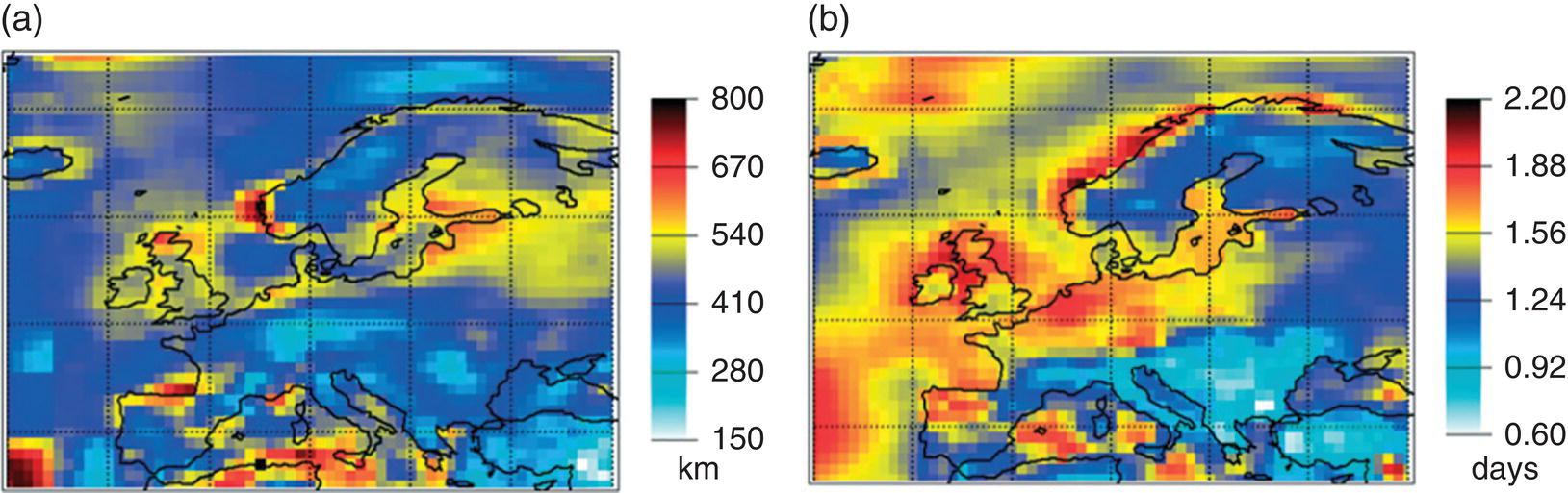
2 Graphical representations of average correlation length (left) and autocorrelation time inferred from ERA‐40 data over a 44‐year period (right) both displaying discrete shaded regions with scale bar for km and days. — **Figure 21.8** (a) Average correlation length and (b) autocorrelation time inferred from ERA‐40 data over a 44‐year period.
Source: Reprinted with permission from Ref.^[82]. Copyright 2008 under the Creative Commons Attribution 3.0 License.

Interannual variability of wind energy has significant implications for the cash flow of a wind farm operator. The year‐ on‐year variation in wind speeds averaged over a number of sites relative to the long‐term mean can be evaluated using a so‐called wind index. For the Nordic countries and the Baltic States^[83], it was shown the standard deviations of the wind indices over the period 1960–1981, normalized to the period 1990–2001, ranged from 8% to 12%, depending on country and reanalysis dataset. For the United Kingdom^[29], the standard deviation of a wind index calculated over 51 years averaged over seven stations was found to be 4% based on surface observations; for a larger sample of 60 stations over a 25‐year period, the standard deviation was found to be 5%. For meteorological stations in Scotland^[30] over a period of 43 years, the interannual change in hypothetical capacity factor was studied, where the capacity factor is defined as the average power output of a wind farm divided by its rated power output over the long term. It was found that the average volatility in wind power output for 10 sites, estimated as the difference between the capacity factor in one year compared with that from the previous year and then normalized by the current capacity factor, was found to be 15%.

Another possibility to reduce the effect of wind power variability is to combine it with other sources of renewable energy generation. The wind and wave power resource around the coast of Ireland was studied^[84], and it was found that west and south coasts of Ireland experience wave conditions that are generated by distant winds far out in the Atlantic, which are little correlated to the wind conditions close to the coast. This provides a good opportunity for co‐located wind and wave power generation whereby combined power output is smoothed. A similar conclusion was drawn for the Californian Coast of the United States^[85], where aggregated power from a co‐located wind and wave farm was found to achieve reductions in variability equivalent to aggregating power from two offshore wind farms approximately 500 km apart or two wave farms, approximately 800 km apart. A study in Denmark looking at optimal combinations for wind, wave, and photovoltaic (PV) power^[86] noted that although the three generation sources were to some extent complementary, this was not a complete solution in terms of integrating variable renewable energy generation.

CONCLUSION

Understanding and managing the variability of the wind will be increasingly important as a larger fraction of electricity is generated by wind farms. The use of the Weibull distribution in estimating expected energy yields is well established, and although there are some sites where it does not fit the observed wind distributions, hybrid bimodal distributions have been shown to perform well. Observations of long‐term wind speeds appear to show that globally, wind speeds are diminishing though this conclusion should be viewed with caution because of inhomogeneities in surface measurements. The conclusions to be drawn from model output such as reanalysis data are less clear, although there is evidence from these for declining wind speeds in some regions. Climate change predictions for changes in wind speed are even more uncertain, and most studies in this area have concluded that any possible climate change‐related signals are smaller than the observed interannual variability. Much research has been done to look at how dispersion of wind farms and increased interconnection could be used to manage variability. It has been concluded that this will help reduce variability, but that there are limits on how well this can help the integration of large amounts of wind power into electricity networks due to the relatively large spatial correlation of wind speeds. Combinations of different renewable generation technologies can play a role, but again, this is not the entire answer.

Looking to the future, more work needs to be done to understand potential long‐term changes in global wind speeds, including mean wind speeds and extremes. In particular, modeling uncertainties need to be reduced if there is to be more confidence in expected future wind speed changes. Modeling of the integration of wind power into networks will need to consider other options to reduce the variable impact of wind power, including the role that can be played by combinations of different renewable generation technologies, demand side management, electric vehicles, and energy storage, along with smarter control of wind farms.

REFERENCES

1. Available at: Global Wind Energy Council Global Wind Report, Annual market update 2011, 2012, http://gwec.net/wp‐content/uploads/2012/06/Annual_report_2011_lowres.pdf. (Accessed March 28, 2013).
2. Van der Hoven, I. (1957). Power spectrum of horizontal wind speed in the frequency range from 0.0007 to 900 cycles per hour. J. Meteorol. 14: 160–164.
3. Smedman‐Hӧgstrӧm, A.‐S. and Hӧgstrӧm, U. (1975). Spectral gap in surface‐layer measurements. J. Atmos. Sci. 32: 340–350.
4. Lovejoy, S., Schertzer, D., and Stanway, J.D. (2001). Direct evidence of multifractal atmospheric cascades from planetary scales down to 1 km. Phys. Rev. Lett. 86: 5200–5203.
5. Bӧttcher, F., Barth, S., and Peinke, J. (2007). Small and large scale fluctuations in atmospheric wind speeds. Stoch. Environ. Res. Risk Assess. 21: 299–308.
6. Laubrich, T. and Kantz, H. (2009). Statistical analysis and stochastic modelling of boundary layer wind speed. Eur. Phys. J. 174: 197–206.
7. Pryor, S.C., Barthelmie, R.J., and Schoof, J.T. (2005). The impact of non‐stationarities in the climate system on the definition of ‘a normal wind year’: a case study from the Baltic. Int. J. Climatol. 25: 735–752.
8. Burton, T., Sharpe, D., Jenkins, N. et al. (2001). Wind Energy Handbook. Chichester, UK: Wiley. ISBN: 0‐471‐48997‐2.
9. Garcia, A., Torresa, J.L., Prietoa, E. et al. (1998). Fitting wind speed distributions a case study. Sol. Energy 62: 139–144.
10. Rehman, S., Halawani, T.O., and Husain, T. (1994). Weibull parameters for wind speed distribution in Saudi Arabia. Sol. Energy 53: 473–479.
11. Celik, A.N. (2003). Energy output estimation for small‐scale wind power generators using Weibull‐representative wind data. J. Wind Eng. Ind. Aerodyn. 91: 693–707.
12. He, Y., Monahan, A.H., Jones, C.G. et al. (2010). Probability distributions of land surface wind speeds over North America. J. Geophys. Res. 115: D04103.
13. Monahan, A.H. and He, Y. (2011). The probability distribution of land surface wind speeds. J. Clim. 24: 3892–3909.
14. Monahan, A.H. (2006). The probability distribution of sea surface wind speeds. Part I: theory and sea winds observations. J. Clim. 19: 497–520.
15. Monahan, A.H. (2006). The probability distribution of sea surface wind speeds. Part II: dataset intercomparison and seasonal variability. J. Clim. 19: 521–534.
16. Bauer, E. (1996). Characteristic frequency distributions of remotely sensed in situ and modelled wind speeds. Int. J. Climatol. 16: 1087–1102.
17. Kozai, K., Ohsawa, T., Takahashi, R. et al. (2012). Evaluation method for offshore wind energy resources using scatterometer and Weibull parameters. J. Energy Power Eng. 6: 1772–1778.
18. Karagali, I., Peña, A., Badger, M. et al. (2014). Wind characteristics in the North and Baltic Seas from the QuikSCAT satellite. Wind Energy 17 (1): 123–140.
19. Coelingh, J.P., van Wijk, A.J.M., and Holtslag, A.A.M. (1996). Analysis of wind speed observations over the North Sea. J. Wind Eng. Ind. Aerodyn. 61: 51–69.
20. Jamil, M., Parsa, S., and Majidi, M. (1995). Wind power statistics and an evaluation of wind energy density. Renewable Energy 6: 623–628.
21. Carta, J.A., Ramírez, P., and Velázquez, S. (2009). A review of wind speed probability distributions used in wind energy analysis: case studies in the Canary Islands. Renewable Sustainable Energy Rev. 13: 933–955.
22. Deaves, D.M. and Lines, I.G. (1997). On the fitting of low mean windspeed data to the Weibull distribution. J. Wind Eng. Ind. Aerodyn. 66: 169–178.
23. Carta, J.A. and Ramírez, P. (2007). Analysis of two‐component mixture Weibull statistics for estimation of wind speed distributions. Renewable Energy 2007: 518–531.
24. Jaramillo, O.A. and Borja, M.A. (2004). Wind speed analysis in La Ventosa, Mexico: a bimodal probability distribution case. Renewable Energy 29: 1613–1630.
25. Carta, J.A. and Ramirez, P. (2007). Use of finite mixture distribution models in the analysis of wind energy in the Canarian Archipelago. Energy Convers. Manage. 48: 281–291.
26. McVicar, T.R., Roderick, M.L., Donohue, R.J. et al. (2012). Global review and synthesis of trends in observed terrestrial near‐surface: implications for evaporation. J. Hydrol. 416–417: 182–205.
27. Greene, S., Morrissey, M., and Johnson, S.E. (2010). Wind climatology, climate change, and wind energy. Geogr. Compass 4/11: 1592–1605.
28. Vautard, R., Cattiaux, J., Yiou, P. et al. (2010). Northern hemisphere atmospheric stilling partly attributed to an increase in surface roughness. Nat. Geosci. 3: 756–761.
29. Watson S J and Kritharas P, 2012. Long term wind speedvariability in the UK. Proceedings of European Wind Energy Association Annual Event, Copenhagen, 16th – 19th April 2012.
30. Früh, W.‐G. (2013). Long‐term wind resource and uncertainty estimation using wind records from Scotland as example. Renewable Energy 50: 1014–1026.
31. Bakker, A.M.R. and van den Hurk, B.J.J.M. (2012). Estimation of persistence and trends in geostrophic wind speed for the assessment of wind energy yields in Northwest Europe. Clim. Dyn. 39: 767–782.
32. Bärring, L. and Fortuniak, K. (2009). Multi‐indices analysis of southern Scandinavian storminess 1780–2005 and links to interdecadal variations in the NW Europe–North Sea region. Int. J. Climatol. 29: 373–384.
33. Wang, X.L., Zwiers, F.W., Swail, V.R. et al. (2009). Trends and variability of storminess in the Northeast Atlantic region, 1874–2007. Clim. Dyn. 33: 1179–1195.
34. Palutikof, J.P., Guo, X., and Halliday, J.A. (1992). Climate variability and the UK wind resource. J. Wind Eng. Ind. Aerodyn. 39: 243–249.
35. Brayshaw, D.J., Troccoli, A., Fordham, R. et al. (2011). The impact of large scale atmospheric circulation patterns on wind power generation and its potential predictability: a case study over the UK. Renewable Energy 36: 2087–2096.
36. Atkinson N, Harman K, Lynn M, et al. 2006 Long‐term wind speed trends in northwestern Europe. Proceedings of the BWEA28 Conference, Glasgow, October 2006 [Internet]. Available at: http://www.gl‐garradhassan.com/assets/downloads/Long_term_wind_speed_trends_in_northwestern_Europe.pdf. (Accessed February 22, 2013).
37. Kalney, E. (1997). The NCEP/NCAR 40‐year reanalysis project. Bull. Am. Meteorol. Soc. 77: 437–471.
38. Uppala, S.M., KÅllberg, P.W., Simmons, A.J. et al. (2005). ERA‐40 re‐analysis. Q. J. R. Meteorolg. Soc. 131: 2961–3012.
39. Pryor, S.C. and Barthelmie, R.J. (2003). Long‐term trends in nearsurface flow over the Baltic. Int. J. Climatol. 23: 271–289.
40. McVicar, T.R., Van Niel, T.G., Roderick, M.L. et al. (2010). Observational evidence from two mountainous regions that near surface wind speeds are declining more rapidly at higher elevations than lower elevations: 1960–2006. Geophys. Res. Lett. 37: L06402.1–L06402.6.
41. Kiss, P., Varga, L., and Jánosi, I.M. (2009). Comparison of wind power estimates from the ECMWF reanalyses with direct turbine measurements. J. Renewable Sustainable Energy 1: 11.
42. Rienecker, M.M., Suarez, M.J., Gelaro, R. et al. (2011). MERRA – NASA's modern‐era retrospective analysis for research applications. J. Clim. 24: 3624–3648.
43. Gunturu, U.B. and Schlosser, C.A. (2012). Characterization of wind power resource in the United States. Atmos. Chem. Phys. 12: 9687–9702.
44. Mearns, L.O., Gutowski, W., Jones, R. et al. (2009). A regional climate change assessment program for North America. EOS 90: 311–312.
45. Greene, S.J., Chatelain, M., Morrissey, M. et al. (2012). Estimated changes in wind speed and wind power density over the western High Plains, 1971–2000. Theor. Appl. Climatol. 109: 507–518.
46. Mesinger, F., DiMego, G., Kalnay, E. et al. (2006). North American reanalysis. Bull. Am. Meteorol. Soc. 87: 343–360.
47. Holt, E. and Wang, J. (2012). Trends in wind speed at wind turbine height of 80 m over the contiguous United States using the North American Regional Reanalysis (NARR). J. Appl. Meteorol. Climatol. 51: 2188–2202.
48. Li, X., Zhong, S., Bian, X. et al. (2010). Climate and climate variability of the wind power resources in the Great Lakes region of the United States. J. Geophys. Res. 115: D18107.
49. IPCC (2000). Special Report on Emissions Scenarios. Intergovernmental Panel on Climate Change. Available at: https://ipcc.ch/pdf/special‐reports/spm/sres‐en.pdf. (accessed 26 March 2013).
50. Solomon S, Qin D, Manning M, et al., eds. 2007 Contribution of Working Group I to the Fourth Assessment Report of the Intergovernmental Panel on Climate Change. Cambridge, UK and New York: Cambridge University Press. Available at: http://www.ipcc.ch/publications_and_data/ar4/wg1/en/contents.html. (Accessed March 26, 2013).
51. Pryor, S.C. and Barthelmie, R.J. (2010). Climate change impacts on wind energy: a review. Renewable Sustainable Energy Rev. 14: 430–437.
52. Harrison, G.P., Cradden, L.C., and Chick, J.P. (2008). Preliminary assessment of climate change impacts on the UK onshore wind energy resource. Energy Sources Part A 30: 1286–1299.
53. Roeckner E, Arpe K, Bengsson L,et al. The atmospheric general circulation model ECHAM‐4: model description and simulation of present‐day‐ climate. Report No. 218, Max Planck Institute for Meteorology, Hamburg, Germany, 1996.
54. Roeckner E, Bauml G, Bonaventura L,et al. The atmospheric general circulation model ECHAM5 part I: model description. Report No. 349, Max Planck Institute for Meteorology, Hamburg, Germany, 2003.
55. Nolan, P., Lynch, P., McGrath, R. et al. (2012). Simulating climate change and its effects on the wind energy resource of Ireland. Wind Energy 15: 593–608.
56. Najac, J., Boé, J., and Terray, L. (2009). A multi‐model ensemble approach for assessment of climate change impact on surface winds in France. Clim. Dyn. 32: 615–634.
57. Najac, J., Lac, C., and Terray, L. (2011). Impact of climate change on surface winds in France using a statistical‐dynamical downscaling method with mesoscale modelling. Int. J. Climatol. 31: 415–430.
58. Breslow, P.B. and Sailor, D.J. (2002). Vulnerability of wind power resources to climate change in the continental United States. Renewable Energy 27: 585–598.
59. Rasmussen, D.J., Holloway, T., and Nemet, G.F. (2011). Opportunities and challenges in assessing climate change impacts on wind energy – a critical comparison of wind speed projections in California. Environ. Res. Lett. 6: 9.
60. Sailor, D.J., Smith, M., and Hart, M. (2008). Climate change implications for wind power resources in the Northwest United States. Renewable Energy 33: 2393–2406.
61. Pryor, S.C. and Barthelmie, R.J. (2011). Assessing climate change impacts on the near‐term stability of the wind energy resource over the United States. Proc. Natl. Acad. Sci. U.S.A. 108: 8167–8171.
62. Pereira de Lucena, A.F., Szklo, A.S., Schaeffer, R. et al. (2010). The vulnerability of wind power to climate change in Brazil. Renewable Energy 35: 904–912.
63. Angeles, M.E., González, J.E., Erickson, D.J. et al. (2010). The impacts of climate changes on the renewable energy resources in the Caribbean region. J. Sol. Energy Eng. 132: 13.
64. Grubb, M., Butler, L., and Twomey, P. (2006). Diversity and security in UK electricity generation: the influence of low‐carbon objectives. Energy Policy 34: 4050–4062.
65. Angarita‐Márquez, J.L., Hernandez‐Aramburo, C.A., and Usaola‐Garcia, J. (2007). Analysis of a wind farm's revenue in the British and Spanish markets. Energy Policy 35: 5051–5059.
66. Swider, D.J., Beurskens, L., Davidson, S. et al. (2008). Conditions and costs for renewables electricity grid connection: examples in Europe. Renewable Energy 33: 1832–1842.
67. Dale, L., Milborrow, D., Slarkc, R. et al. (2004). Total cost estimates for large scale wind scenarios in UK. Energy Policy 32: 1945–1956.
68. Holttinen H. 2006 Handling of wind power forecast errors in the Nordic power market. Proceedings of Probabilistic Methods Applied to Power Systems, Stockholm, Sweden 11–15 June 2006.
69. Holttinen H. Meibom, P. and Orths, A. et al. Design and operation of power systems with large amounts of wind power. Final Report, IEA WIND Task 25. Phase one 2006–2008. ISBN 978–951‐38‐7308‐0, published by VTT, Technical Research Centre of Finland. Available at: http://www.vtt.fi/inf/pdf/tiedotteet/2009/T2493.pdf. (Accessed March 28, 2013).
70. Chang, J., Ummels, B.C., van Sark, W.G.J.H.M. et al. (2009). Economic evaluation of offshore wind power in the liberalized Dutch power market. Wind Energy 12: 507–523.
71. Hartnell, G. (2000). Wind on the System – Grid Integration of Wind Power. Renewable Energy World. London: James and James (Science Publishers) Ltd.
72. Purvins, A., Zubaryeva, A., Llorente, M. et al. (2011). Challenges and options for a large wind power uptake by the European electricity system. Appl. Energy 88: 1461–1469.
73. Degeilh, Y. and Singh, C. (2011). A quantitative approach to wind farm diversification and reliability. Electric. Power Energy Syst. 33: 303–314.
74. Caralis, G., Perivolaris, Y., Rados, K. et al. (2008). On the effect of spatial dispersion of wind power plants on the wind energy capacity credit in Greece. Environ. Res. Lett. 3: 13.
75. Drake, B. and Hubacek, K. (2007). What to expect from a greater geographic dispersion of wind farms?—a risk portfolio approach. Energy Policy 35: 3999–4008.
76. Katzenstein, W., Fertig, E., and Apt, J. (2010). The variability of interconnected wind plants. Energy Policy 38: 4400–4410.
77. Pestana R. 2008 Dealing with limited connections and large installation rates in Portugal. The 2nd Workshop on Best Practice in the Use of Short‐term Forecasting, Madrid, Spain, 28 May 2008. Available at: http://powwow.risoe.dk/publ/RPestana_(REN)‐DealingWLimitedConnALargeInstallRatesInPT_BestPractice STP‐2_2008.pdf. (Accessed July 9, 2013).
78. Giebel G. 2000 On the benefits of distributed generation of wind energy in Europe. PhD Dissertation, Carl von Ossietzky University, Oldenburg, 2000, (104). Available at: http://www.drgiebel.de/GGiebel_DistributedWind EnergyInEurope.pdf. (Accessed March 28, 2013).
79. Fertig, E., Apt, J., Jaramillo, P. et al. (2012). The effect of long‐distance interconnection on wind power variability. Environ. Res. Lett. 7: 6.
80. Kempton, W., Pimenta, F.M., Veron, D.E. et al. (2010). Electric power from offshore wind via synoptic‐scale interconnection. Proc. Natl. Acad. Sci. U.S.A. 107: 7240–7245.
81. Hasche, B. (2010). General statistics of geographically dispersed wind power. Wind Energy 13: 773–784.
82. Kiss, P. and Jánosi, I.M. (2008). Limitations of wind power availability over Europe: a conceptual study. Nonlinear Processes Geophys. 15: 803–813.
83. Pryor, S.C., Barthelmie, R.J., and Schoof, J.T. (2006). Inter‐annual variability of wind indices across Europe. Wind Energy 9: 27–38.
84. Fusco, F., Nolan, G., and Ringwood, J.V. (2010). Variability reduction through optimal combination of wind/wave resources – an Irish case study. Energy 35: 314–325.
85. Stoutenburg, E.D., Jenkins, N., and Jacobson, M.Z. (2010). Power output variations of co‐located offshore wind turbines and wave energy converters in California. Renewable Energy 35: 2781–2791.
86. Lund, H. (2006). Large‐scale integration of optimal combinations of PV, wind and wave power into the electricity supply. Renewable Energy 31: 503–515.

Table of Contents for
21 Quantifying the Variability of Wind Energy

21
Quantifying the Variability of Wind Energy

THE IMPORTANCE OF WIND VARIABILITY

AN OVERVIEW OF DIFFERENT SCALES OF VARIABILITY

WIND SPEED DISTRIBUTIONS