
29
Multivariate Analysis of Solar City Economics: Impact of Energy Prices, Policy, Finance, and Cost on Urban Photovoltaic Power Plant Implementation
John Byrne1,2, Job Taminiau1,2, Kyung N. Kim3, Joohee Lee1 and Jeongseok Seo1
1 Center for Energy and Environmental Policy, University of Delaware, Newark, DE, USA
2 Foundation for Renewable Energy & Environment, New York, NY, USA
3 Green School, Korea University, 145, Anam‐ro, Seoul, South Korea
Previous research suggests that the potential for city‐scale photovoltaic (PV) applications is substantial across the globe. Successful implementation of “solar city” options will depend on the strategic application of finance mechanisms, solar energy soft cost policies, and other policy tools, as well as the grid price of electricity. Capital markets recently have embraced the roll‐out of new financial instruments, including “green bonds,” which could be incorporated into solar city project design to attract large investments at a low cost. A multivariate analysis method is employed to consider solar city possibilities for six cities: Amsterdam, London, Munich, New York, Seoul, and Tokyo. A Monte Carlo simulation is conducted to capture the probabilistic nature of uncertainties in the parameters and their relative importance to the financial viability of a solar city project. The analysis finds that solar city implementation strategies can be practical under a broad range of circumstances.
INTRODUCTION
The December 2015 Paris Climate Agreement signals a new direction for global climate change. For the first time, commitments by nearly all countries have been agreed upon. While the scale of required change sizably surpasses these commitments, the Paris Agreement has the distinct advantage of directing attention to implementation rather than policy design. In this vein, a critical challenge is the immaturity of the renewable energy sector as a target for city‐scale development. Investing in renewable energy still focuses mainly on individual, modestly sized projects. For instance, solar electric power typically attracts investments in a few hundred kWp to tens of MWp. A growing number of policy analysts and technology researchers argue that a new focus is needed on infrastructure‐scale planning to advance low carbon energy transitions[1, 2].
At the same time, experience shows that infrastructure investment must respond to context‐ and location‐specific factors, leading many to emphasize a post‐Paris “polycentricity paradigm” in climate change governance and economics where policy, planning, and strategy is operationalized by nation–state, regional, city, and city network initiatives[3]. Cities, in particular, have positioned themselves as champions of sustainable energy change, combining their efforts in transnational networks and collaboration[4].
To that end, this chapter explores the possibility for cities to engage in network‐wide climate change strategies to attract capital market attention through capitalization of existing and currently unutilized rooftop real estate that is abundant in the urban environment. Termed “solar cities,” such strategies use city governance vehicles to catalyze public sector‐led, infrastructure‐scale design and investment of city‐wide photovoltaic (PV) technology deployment. Successful access to capital markets could increase the scale and speed of solar deployment[5]. For instance, city‐scale implementation efforts could benefit from the rising prominence of “green bonds,” “climate bonds,” and other financing innovations that have been able to expand large‐scale capital investments for green purposes[2]. Global issuance as of August 2016 (i.e. 9 months of investments) stands at $46.03 billion, or $5 billion more than investments in all of 2015.1 The emerging financial instrument could be a promising vehicle for solar city strategies: incorporating public debt in the financing structure offers attractive benefits such as improvements in financing terms, risk mitigation, and access to a broader capital pool[6]. Overall, such strategies could achieve a lower cost of capital, less risk, and reduce project costs[7, 8]. It is estimated that a reduction in the levelized cost of energy (LCOE) of 8–16% occurs when a portion of a project or portfolio's typical capital stack is replaced with public capital vehicles[5].
This study advances earlier work from Ref.[2] by introducing a multivariate analysis method for assessing solar city economics in the same six cities studied in the previous publication: Amsterdam, London, Munich, New York City, Seoul, and Tokyo. The analysis is organized in five steps. After reviewing newly published work in the field, which points to significant untapped potential (Brief Review of Recent “Solar City” Assessment Literature section), the paper describes a multivariate method to evaluate solar city economics (Analytic Approach section). The next section covers a project finance analysis of data to illustrate the relative impacts of market, finance, and policy portfolios in solar city economics (Project Finance Analysis section). Using regression analysis, the variables driving solar city viability are assessed (Regression Results section), and the model is evaluated using statistical tests for robustness and validity (Model Robustness Tests section). Conclusion section concludes that city‐scale applications are practical – the necessary policy tools exist and have been shown to work, and the economics and financeability of such projects are affordable.
BRIEF REVIEW OF RECENT “SOLAR CITY” ASSESSMENT LITERATURE
The latest modeling assessments and other research continue to strengthen the case for urban “solar city” applications, where urban energy economies are retooled toward a strong reliance on PV energy generation using the large rooftop area available to cities[2, 9]. Research regarding urban applications of PV has addressed, with growing sophistication, methodological issues in determining the overall technical potential of PV in cities[10, 11]. Such investigations have been performed for a wide variety of urban conditions ranging from cities in Nigeria[12] to India[13], Abu Dhabi[14], the Netherlands[15], the United States[16, 17], and Brazil[18].
Studies typically find considerable potential for urban deployment of PV. For example, Gagnon et al.[16] calculate that the suitable rooftop space in the state of California can generate 74% of the electricity sold by utilities in 2013, while several New England states are found to be able to generate over 45% of their electricity needs by utilizing existing rooftop area. At the national level, Gagnon et al.[16] estimate that rooftop solar power could generate 38.6% of national electricity demand, and similarly, at the city level, cities like Los Angeles (60% of electricity needs), San Francisco (50%), Miami (46%), and Atlanta (41%) show substantial potential.2 Gagnon et al.[16] performed their calculation for 47 cities across the United States and found that, collectively, these cities have the technical potential to host an impressive 84.4 GWp of solar capacity – the Solar Energy Industry Association (SEIA) puts the current total US‐installed PV capacity at about 25 GWp[19]. Los Angeles (9 GWp), New York City (8.6 GWp), and Chicago (6.9 GWp) combined could match current US‐installed capacity.
Other dimensions of solar energy potential modeling have been explored by looking at, e.g. a variety of rooftop technologies[20], different configurations of urban morphology[21, 22], varying system design considerations[23], optimization opportunities[24], or possible interaction patterns with mobility options[25].
The practical implementation of solar cities as an adaptive strategy available to local policy makers, however, remains limited. While there is value in further discussion and research regarding methodology refinement, research targeting the practicality of the solar city concept as a city‐wide strategy is timely and necessary to advance the field. An earlier attempt to do so introduced the policy, market, and finance implications associated with solar city strategies[2].
ANALYTIC APPROACH
The examination of solar city's practicality relies on three analytical tools: (i) project finance analysis, (ii) regression analysis, and (iii) robustness tests. Each is described in this section and then applied in the following sections.
Benefit‐Cost Analysis
A first assessment of project viability is to determine the benefit cost ratio in the first year of the project (Eq. (29.1)) and the benefit cost ratio in the year the debt matures (Eq. (29.6)). Calculations and analysis were performed using the System Advisor Model (SAM) software developed at the National Renewable Energy Laboratory (NREL) in the United States. All dollar amounts are in nominal dollars.
where n = year of the project. The other variables given in Eq. (29.1) are further defined in Eqs. (29.2)–(29.5).

The output factor (OF) in kWh/kWp refers to the combined effect of the typical meteorological year output data that is specific to the meteorology of the geographical location, PV system characteristics (e.g. module efficiency, tilt, etc.), and morphological conditions of the city in question. See Table 29.1 for the OF of each location.
Table 29.1 Overview of the input data.
| City | Output factor (kWh/kWp) | Electricity retail rate ($/kWh) | Policy benefits ($/kWh) | Hard costs ($/kW) | Soft costs ($/kW) | Capital costs (interest rate) (%)a |
| AMS | 967 | 0.148 | 0.114 | 1498 | 642 | 1.8 |
| LON | 979 | 0.167 | 0.16 | 1530 | 1020 | 3.6 |
| MUN | 1079 | 0.208 | —b | 1435 | 615 | 1.5 |
| NYC | 1364 | 0.224 | 0.099c | 2046 | 1674 | 3.1 |
| SEOUL | 1110 | 0.116 | 0.127 | 1470 | 980 | 3.5 |
| TOKYO | 1218 | 0.194 | 0.077 | 2154 | 1436 | 0.6 |
Explanation about data and data sources provided in Byrne et al.[2].
a Capital costs given in Table 29.1 are for a 10‐year bond offering. Interest rates differ per bond maturity; relationship of change in the form of yield curves is provided by Byrne et al.[2].
b Recent changes to the German renewable energy support structure are an example of the uncertainty developers and investors can face. Policy changes to reduce feed‐in tariff payments are one factor contributing to a recent decline in German PV installations from 2013s 3.3 GWp to 1.4 GWp of new capacity in 2015. This installation level is down from the 7.5 GWp installed annually in 2010, 2011, and 2012[31, 77]. Of course, other factors played a role in this decline, but the policy decision (as part of a “third phase” in the German “Energiewende”) to recognize rapidly falling technology costs and a maturing market was important. The third phase of implementation reflects the view that “grid parity” is in sight, and efficient deployment of solar PV can be achieved at lower levels of policy support[78]. Munich's policy support is set at zero by the authors in light of the recent decision by the government to significantly reduce its incentive programs. In this way, the results reported here reflect a robust range of scenarios where significant policy support is present and where policy support has been removed.
c For New York City, the capital‐based incentive is calculated as a production‐based compensation for a 10‐year period for comparison.
The degradation rate (DR), in percent, accounts for system losses over time and is set at 0.5% across all locations following Ref.[26].
The electricity rate (ER), in cents/kWh, is the administratively set commercial ER that is applicable in the case study city as an approximate measure of the value of electricity generated by the PV power plant.3 See Table 29.1 for the ER of each location.
The electricity growth rate (EGR), in percent, reflects the expected growth pattern of the ER. The EGR is set at 2% in each location.
Policy support refers to the existing policy conditions to support PV generation in each city, including the national policy system, which are described in detail in Ref.[2]. Policy support value is assumed to be in place for 10 years, after which it is eliminated. Policy support values are presented in Table 29.1 for each location.

Following Ref.[2], the OM constant was set at $25.0/kWp,4 and inflation (i) is set at 2% for each location.

Debt service (DS) refers to the constant periodic payment required to pay off the capital investment, both “soft” and “hard” costs (see below), with a constant interest rate (IR) over a specified period (MAT). DS is calculated using EXCEL's PMT function that combines IR, principal (HC and SC), and maturity (MAT).5
Byrne et al.[2] previously considered project viability in a relatively straightforward manner: solar cities were assessed to be viable if annual benefits (derived from both policy support and energy sales) were higher than annual costs (consisting of investment, operation and maintenance, and interest) for all years of the project's lifetime (assumed to be 25 years). An important variable over the lifetime of the project is the duration of policy support: policy benefits (PBs) typically expire before the end of the technical lifetime of the project. This variable must rely on an assumption regarding their expiration. In the 2016 article by Byrne et al., a 10‐year retirement was assumed and is repeated here. However, this treatment can cause annual costs to be higher than annual benefits for a short period of time right after PB expiration, threatening project viability. Despite substantial positive cash flows for the first 10 years of city projects, long financing maturities were required to overcome this obstacle. However, such shortfalls can be brief and small compared to the surplus generated in the first 10 years of the projects. For this reason, project viability is redefined in this analysis to be based on cumulative cash flow: city projects are viable if cumulative cash flow is positive throughout the lifetime of the project. Using the same terms as above, but including a cost and price escalator of 2% and PV system performance degradation of 0.5%, the cumulative benefit‐to‐cost ratio determines the project viability for a 25‐year PV installation (Eq. (29.6)).
Key model input variables that are subject to variability tests (described below) are provided in Table 29.1 for each city. Variability in investment conditions can substantially alter the risk profile of renewable energy:
- Policy changes. Policy support uncertainty can reduce investor confidence and limit investment[27–30]. Recent examples of such policy uncertainty are the retroactive modification of Spain's feed‐in tariff and Germany's substantial lowering of its price premium[29, 31].
- Financing period. In response to a “mock” solar securitization filing, US rating agencies indicated that the typical 20‐year contract lifetime for PV projects is unlikely to remain as the market matures and proposed 7‐ to 10‐year maturities as a more reasonable timeframe for analysis purposes[32].
- Cost of capital. The absence of performance data regarding infrastructure‐scale PV securitizations fuels a cyclical phenomenon where “risk perception is fed by lack of historical knowledge, which is in turn fed by risk perception[33].” As such, “it may be realistic to assume that the first securitizations will not obtain an optimal spread between the cost of capital of securitization debt and, say, that of a commercial loan[6].” Credit enhancement techniques, such as overcollateralization, first‐loss reserves, or tranching can, on the other hand contribute to lowering the cost of capital[6, 33].
- PV system output. The output function of a solar PV system is dependent on a wide range of underlying variables. For instance, system performance is determined by meteorological conditions, urban morphology, module efficiency, angular deployment of PV panels, system performance degradation, PV technology choice, and shading (e.g. from other rooftop obstacles, from other buildings, or panel‐to‐panel shading). Urban morphology conditions are particularly different across locations and range from macro‐scale to micro‐scale elements: city districts (e.g. comparing a business district against a suburban neighborhood) provide different shading conditions, different heating/cooling requirements, or are subject to different fire codes, and similarly, individual buildings can be designed specifically with PV in mind or be ornate and largely unsuitable for PV deployment[21, 22, 34]. By relying on the modification of six variables, such as the amount of open space, the closeness of buildings, and the standard deviation of building heights, certain building design changes could improve London's rooftop PV performance by about 9% while enhancing façade profiles by 45%[22]. A study of New York's Battery Park commercial district (a vertical, high‐density area) shows annual rooftop solar irradiation variability from 1200 to 1350 kWh m−2 – or about 6.4–16.8% lower compared to the unobstructed annual irradiation level[35].
- Technology and market dynamics. Solar electric power generation technologies have experienced a dramatic drop‐off in overall costs[36]. However, while median prices of solar power have steadily declined, significant variability in the cost of both rooftop and commercial‐scale solar installations remains. For instance, in the United States, the price point difference between the 20th percentile and 80th percentile is $1.7/Wp for residential and $1.6/Wp–$1.3/Wp for nonresidential systems[36]. Moreover, dominant market relations, geographic market conditions, and contractual arrangements influence the pattern of technology price development (e.g. by affecting feedstock trade flows or costs)[37]. Price and cost volatility characterizes the learning curve of PV[38]. Also, as prices come down for some components, other components or aspects become more prominent in future prices[39, 40]. A particular distinction can be made between the “hard” and “soft” cost patterns of PV, and a discussion on this balance in each location is provided below.
Hard Costs Versus Soft Costs
Overall, “hard” costs of solar electric power, particularly PV module prices, have fallen dramatically[36]. For instance, module prices fell by $2.7/Wp (2014 dollars) over the 2008–2012 period[36]. Nonmodule cost improvements, however, have also contributed to a continuing decline in installed costs[41]. For example, since 2009, nonmodule costs have decreased by 10% year‐over‐year and contributed to a $0.4/W decline in cost from 2013 to 2014[36]. Key contributors to these price reduction patterns are lower costs for inverters and racking equipment and falling average generation costs due to increasing system size and module efficiency[36, 42]. However, increasing scrutiny directed toward “soft” costs, such as permitting, regulatory context, marketing, customer acquisition, installer margins, installation labor, and system design, has likely also contributed to installed cost reductions for PV[21].6
Recent research into PV‐installed costs has focused on so‐called “soft costs,” e.g. Refs.[44–50]. Considering hardware costs are “fairly similar” across countries, soft cost profiles can be a key differentiator in installed costs[51]. Soft cost “best practices” can significantly reduce overall costs, e.g. Ref.[47]. Importantly, soft costs in the German system are about 50% lower than the United States[47], in large part because the former has standardized both the design approval and permitting processes. For instance, the difference between the United States and Germany is striking: the feed‐in tariff registration form, which enables grid‐connected solar residences to receive federal incentives, is the only German paperwork required for PV systems. Typically, this form takes as little as five minutes to fill out and is conveniently submitted online. In contrast, most US [ jurisdictions] require a combination of engineering drawings, building permit, electrical permit, design reviews, and multiple inspections before approving a PV installation (Ref.[39]).
Differences in soft costs occur within, as well as across, countries. A recent analysis of US soft costs found an 8–12% reduction potential for a highest‐scoring municipality compared to the lowest‐scoring soft cost community[49]. Similarly, Dong and Wiser find that the most favorable permitting practices in cities in California resulted in reductions of $0.27–$0.77/Wp lower costs (4–12% of median California price points) compared to cities with the least favorable permitting practices[52]. Researchers have also found that regulatory and policy barriers that affect soft costs in some cases would lead installers to avoid certain jurisdictions[53, 54].
Establishing specific soft costs at the city level requires an investigation into factors such as permitting, installation labor, margins, etc. that is beyond the scope of the present research. Instead, we focus on the ratio between soft and hard costs for each city as determined by extant literature. National‐level data are used where available and extrapolated to neighboring countries where local data are unavailable.
Soft costs have been extensively studied in the United States, e.g. Refs.[44–49, 55]. The results point to a substantial potential in installation cost reduction as soft costs make up a significant share of total installed costs. For instance, in the first half of 2012, soft costs made up 64% of the total US residential installed cost, 57% of US small commercial, and 52% of US large commercial projects[53]. Similar results were produced in a more recent investigation: 55% of residential costs were attributable to soft costs, commercial projects devote 42% of installation costs to soft costs, and utility‐scale projects must cover 34–36% in soft costs[45]. In the analysis presented here, we assume that New York City's installation cost is made up of 45% soft costs and 55% hard costs. This assumption is similar to the ratio for commercial projects in the United States, a reasonable facsimile for our solar city buildout on New York's rooftops.
The extant literature commonly points to Germany as an example of best practices in terms of soft costs[39, 56]. Research has been particularly directed toward the soft cost profiles of the residential market. For instance, Seel et al.[47] compare soft costs between Germany and the United States and find that soft cost differences for residential systems amounted to $2.72 W−1 in 2011–2012. This means a doubling of soft cost payments in the United States – Germany spends 21% of a residential system installation ($0.62/W) on soft costs compared to 54% in the United States ($3.34 W−1)[47]. A separate analysis by the German solar energy association finds that just over 31% of a commercial application of rooftop solar energy can be attributed to soft costs, and a recent study by the Fraunhofer Institute uses 30% for this cost element[57].7 For these reasons, we assume a 70% module and hard cost and 30% soft cost profile for the City of Munich.
A recent publication found a similar difference in cost between Japan and the United States[46]. Hard costs, particularly module costs, are $0.67 W−1 higher in Japan compared to the United States, leading to a different soft cost/hard cost balance: soft costs account for about 44% of residential and 39% of small commercial system costs in the first half of 2013[46]. This finding is further supported by data from the International Energy Agency (IEA) Photovoltaic Power Systems Programme (PVPS) for Japan[58]. The inputs for Tokyo used here are, therefore, that soft cost prices make up 40% of system price, while hard costs make up 60%. This puts Tokyo in between Germany and the United States in terms of the proportion of installed costs dedicated to the soft, downstream elements of the value chain.
Detailed soft cost versus hard cost breakdowns for other countries remain to be investigated. We assume here that Amsterdam has a similar profile to Munich,8 London has a similar profile as New York City,9 and Seoul has a similar profile as Tokyo.10 The inputs for soft cost versus hard cost are provided in Table 29.2.
Table 29.2 Inputs for hard and soft cost percentage for each city in the analysis.
Source: Based on national data reported by Refs.[25, 36, 39, 45, 55] and extrapolations where national data are unavailable.
| City | Hard costs (%) | Soft costs (%) low soft costs |
| Amsterdam | 70 | 30 |
| Munich | 70 | 30 |
| Medium soft costs | ||
| Seoul | 60 | 40 |
| Tokyo | 60 | 40 |
| High soft costs | ||
| New York City | 55 | 45 |
| London | 55 | 45 |
Monte Carlo Simulation
Because full‐scale solar city implementations have yet to occur, a Monte Carlo simulation approach was used to test the impact of variability and to illustrate the consequences of uncertainty. Probabilistic analysis techniques represent a suitable tool for this task[64–66]. Monte Carlo simulation is a well‐recognized method, and the analysis below parallels its application performed in other studies, e.g. Refs. [64, 67, 68]. Input variable sampling is carried out by using a random number generator within a preselected input variability range. Repeating the procedure for a large number of simulations generates a density function for the model output values. The calculated output (see Benefit–Cost Analysis section) is conducted for each input variable separately to simulate the possible solar city economics faced by local governments in the selected locations. The approach is illustrated in Figure 29.1.
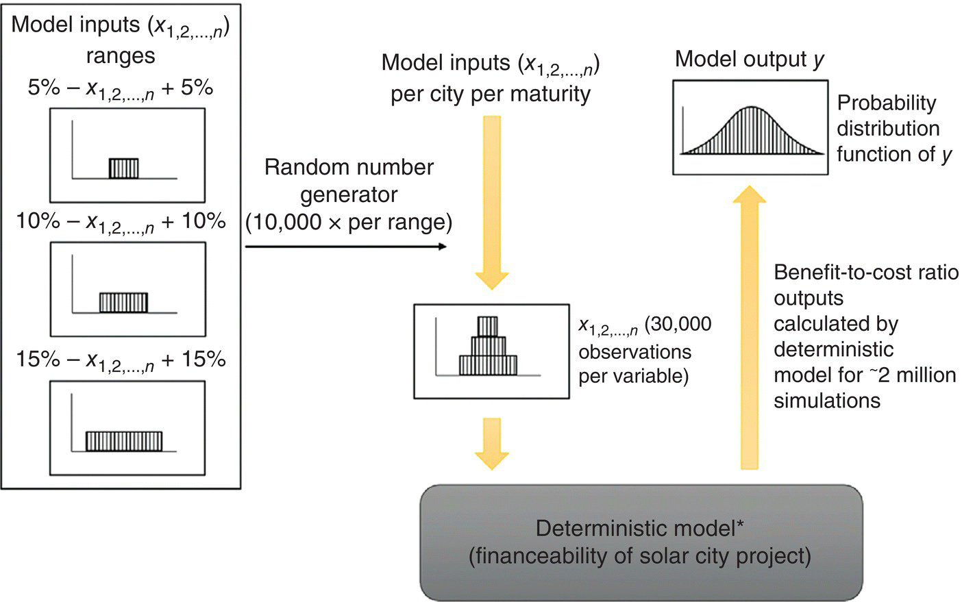
Figure 29.1 Monte Carlo assessment of project finance. *NREL's System Advisor Model (SAM) is used to calculate the benefit–cost ratios (https://sam.nrel.gov).
To test solar city financeability more robustly, the Monte Carlo assessment was performed for ±5%, ±10%, and ±15% changes in the input variables. The input variables selected to be subject to this range of change were: (i) bond capital costs, (ii) the electricity retail price at the moment of bond issue for which solar generated electricity can be sold, (iii) the rate of change in electricity retail price over time, (iv) the “hard” and “soft” costs of the PV system, and (v) the level of policy support (see below for statistical justification of the selected variables). The analysis was conducted across bond issue maturities from 6 to 16 years, with 10 000 simulations created for each variability range (i.e. ±5%, ±10%, and ±15%), each maturity, and for each city to ensure random selection of benefit‐to‐cost ratios. This maturity range was selected to encompass the suggested timeframe by rating agencies of 7–10 years (see Ref.[32]) and include the high end of financial feasibility uncovered by Ref.[2]. Across three ranges of variability – 6 cities and 11 maturities – the Monte Carlo assessment yields a total of just under 2 million simulations.
Regression Analysis
Our next step was to build a multiple regression model to determine the ability of each input factor to predict solar city benefit‐cost ratios. The analysis ranks cost and benefit inputs according to the magnitude and sign of standardized regression coefficients (SRCs)[69].11 This statistical approach allows for the quantification of predictors and a ranking of their relative importance in determining cumulative benefit‐to‐cost ratios. A regression analysis was conducted for each city individually, for each maturity, and for all cities combined for each maturity. We used EViews Version 8.1 software to run the calculations (http://www.eviews.com).
The independent variables used for the analysis were: (i) the IR charged on the bond offering, (ii) the hard costs of the installation (HC), (iii) the soft costs of the PV installation (SC), (iv) the OF of the system (OF), (v) the PBs offered in each location (PB), (vi) the growth rate of the retail electricity price throughout the bond offering (i.e. the price escalator; EGR), and (vii) the commercial retail rate in each location (ER). Monte Carlo variations in each of these model inputs were used to determine the benefit‐to‐cost ratio in the year of maturity (i.e. at the conclusion of the financing round) as the dependent variable (see Eq. (29.1)). The relationship is described in Eq. (29.7), with an error term u.
Standardization of the regression is described in Eq. (29.8). Standard errors for the βs in Eq. (29.8) are based on White's heteroscedasticity‐consistent standard error formula[70] using the function provided by the Eviews Version 8.1 software.
Model Robustness Check
Graphical model validation checks were carried out to evaluate the performance of the model. In particular, the distribution of the residual errors offers insight into the functioning of the regression model. In addition, using three different variability ranges (±5%, ±10%, and ±15%) adds to the understanding of the robustness of the model.
PROJECT FINANCE ANALYSIS
Two cities – New York and Munich – have financially viable solar city investment opportunities regardless of variability in input values (Figure 29.2). As depicted in Figure 29.2, illustrating the comprehensive results of the Monte Carlo assessment with combined variability in input data of ±5%, ±10%, and ±15%, New York, for any maturity greater than 12 years, can confidently expect a benefit‐to‐cost ratio greater than 1.0. In Munich's case, this point is reached for maturities equal to or greater than 13 years. For New York and Munich, 90% of the simulations for the combined variability scenarios show ratios greater than 1.0 from, respectively, 12 and 13 years onward.

Figure 29.2 Results of the Monte Carlo analysis using a 90% interval around the mean for each city for a combined variability of the input data. Notes: Combined variability is achieved by varying input data by ±5% for 10 000 simulations per maturity year, ±10% for 10 000 simulations per maturity year, and ±15% variability for another 10 000 simulations per maturity year. A total of 30 000 simulations, therefore, are assessed to determine the benefit–cost ratios. The mean and 90% range correspond with the left y‐axis, and the columns correspond with the right y‐axis, depicting the percentage of simulations that are defined as viable projects (i.e. positive cumulative benefit cost ratios in all years of the project, using Eq. (29.6)). The distinctive “bend” in the results is a direct effect of the assumed 10‐year lifespan of the policy benefits in each location: as soon as the policy benefits expire, the benefit‐to‐cost ratio relies solely on the retail electricity rate and electricity growth rate to determine the benefits component of the analysis. A gradual phase‐out of the policy benefits or other mitigating strategies could shorten the required financing timeframe.
In a second tier of investment opportunities, Amsterdam, London, and Tokyo need longer to realize financeability; all appear financeable with maturities of 16 years. The cumulative benefits of solar city investments in the three cities exceed, or are very close in exceeding, all costs in 90% or more of the simulations when the financing can be stretched over 16 years. Amsterdam, London, and Tokyo reach a mean benefit‐to‐cost ratio larger than 1.0 under 11‐, 12‐, and 13‐year financing maturities, respectively.
The third tier, consisting of the City of Seoul, cannot confidently offer net positive investment opportunities (defined as the point at which 90% of the simulations have cumulative net positive cash flows) when cost input variability can be as high as +15%. Seoul's solar city investment achieves positive cash flow only for a small share of the 30 000 simulations under 16‐year financing conditions. As discussed below, a key barrier is its grid price, which the national government sets administratively. The current price is 3.2–10.8 cents lower than its five counterparts.
REGRESSION RESULTS
The analysis was conducted for both each city individually for each maturity and for all cities combined for each maturity.
Regressions by City
We were able to identify predictor structures for each of the six cities. These are reported in Table 29.3. For New York, the high electricity retail rate delivers a substantial contribution to the financial viability of its solar city project. In contrast, the low electricity retail rate in Seoul (the lowest in the sample of cities) is the key impediment to financial viability of the project.
Table 29.3 Overview of regression results by city.
| Variable | Standardized regression coefficient | |||||
| Amsterdam | London | Munich | New York | Seoul | Tokyo | |
| Interest rate | −0.0591 | −0.1184 | −0.0484 | −0.0860 | −0.1133 | −0.0211 |
| Hard costs | −0.4428 | −0.3933 | −0.3955 | −0.3040 | −0.3890 | −0.3842 |
| Soft costs | −0.1888 | −0.2628 | −0.1694 | −0.2510 | −0.2611 | −0.2561 |
| Output factor | 0.7023 | 0.7088 | 0.6343 | 0.6055 | 0.7066 | 0.6839 |
| Policy benefit | 0.2753 | 0.3132 | — | 0.3032 | 0.3346 | 0.1685 |
| Electricity growth rate | 0.0402 | 0.0362 | 0.0578 | 0.0555 | 0.0348 | 0.0466 |
| Electricity rate | 0.4287 | 0.3994 | 0.6344 | 0.6077 | 0.3758 | 0.5151 |
| R 2 | 0.9954 | 0.9954 | 0.9947 | 0.9937 | 0.9955 | 0.9951 |
Results are provided for a 10‐year maturity schedule. Interest rate and electricity growth rate variables show the most change with changes in maturity schedule (longer maturity schedules make these variables more important). The policy benefit variable shows a higher level of change after 10‐year maturity (benefits are assumed to expire after 10 years). Yet, the relative position of variables remains regardless of maturity schedule. Germany has substantially lowered its policy incentive programs, and as a result, Munich's regression was run without this variable.
Other findings include:
- Borrowing IRs have minor influence on financial viability compared to the other factors. This finding holds across all locations. However, in terms of policy strategies and options to increase the viability of a solar city project, developers might have some control over the cost of finance, e.g. by focusing on a socially responsible or “impact” investor base.
- Price developments throughout the project appear to have a modest effect on project viability. Unsurprisingly, changing the price point at which the generated electricity is sold has a substantial effect on PV competitiveness.
- The relative influence of soft costs in Amsterdam and Munich, two cities where substantial progress on soft cost improvements has already taken place, is also modest. The relative influence of the variable is more pronounced in some of the other locations.
Overall, predictors had the expected signs, and a common predictor structure can be uncovered. Using standardized heteroscedasticity robust coefficients to define variable contribution, the system OF variable has the greatest predictive impact on project financial viability. Retail ERs are the second most influential factor in contributing to positive benefit‐cost ratios. Solar panel costs (HC) have the largest negative influence on project cash flows. Although its predictive power varies due to differences among the cities and the national commitments that underpin local efforts, the importance of PBs is evident. The common predictive structure and variation in influence of the variables is captured in Figure 29.3.

Figure 29.3 Multivariate regression results for each city for the seven variables. Notes: For each city, the ranking of the coefficients shows the influence of that variable on the benefit–cost ratio. Generation potential (kWh m−2) and the electricity retail rate are the key drivers of benefit–cost ratio outcomes in most locations. A notable exception is the City of Seoul where the electricity retail rate is relatively less important due to its low starting point.
Regression Analyzing the Combined Pool of Cities
Conducting the regression analysis across the pool of six cities shows that the electricity retail rate is the largest factor affecting positive cash flow, with solar radiation a very close second factor. Because of large differences in city/national SC policies, it ranks as a more prominent factor compared to solar panel costs in shaping overall project cost (Table 29.4).
Table 29.4 Overview of the regression results of the combined regression analysis.
| Variable | Standardized regression coefficient IR |
| IR | −0.4083 |
| HC | −0.7950 |
| SC | −0.9381 |
| EGR | 0.0334 |
| OF | 1.0677 |
| ER | 1.3070 |
EGR, electricity growth rate; ER, electricity rate; HC, hard costs; IR, interest rate; OF, output factor; SC, soft costs.
Numbers provided here are for a 10‐year maturity schedule of the debt. Interest rate and electricity growth rate variables show the most change with changes in maturity schedule (longer maturity schedules make these variables more important). Yet, the relative position of variables remains regardless of maturity schedule.
The regression analysis across the pool of six cities further allows for the calculation of the relative value of PBs across locations (Table 29.5). The viability of London and Seoul's solar projects are comparatively more dependent on policies in place in their markets, while the projects of Amsterdam, New York City, and Tokyo are less dependent. The third column in the table offers a brief explanation of the relative ordering of the cities.
Table 29.5 Overview of the PB in each location.
| City | PB standardized regression coefficient | Comparative PBs |
| Munich | — | No PB needed, PV market ready |
| Tokyo | 0.7328 | Low PB, high reliance on market factors |
| New York City | 1.1069 | Capital PB, high electricity price |
| Amsterdam | 1.1434 | Moderate PB, moderate electricity price |
| Seoul | 1.2574 | Considerable PB, low electricity price |
| London | 1.4258 | High PB, moderate electricity price |
PB, policy benefit.
Results are provided for a 10‐year maturity schedule. The PB variable shows a higher level of change after 10‐year maturity (benefits are assumed to expire after 10 years). Yet, the relative position of variables remains regardless of maturity schedule.
RESULT OF THE MODEL ROBUSTNESS CHECK
The very large sample sizes provided by the Monte Carlo simulation (180 000 simulations in the analysis of combined samples) make the typical normality tests unhelpful here as these tests are intended for assessments involving smaller sample sizes (typically less than 50 cases). Instead, model validation was considered by using graphical tools. A histogram eyeball test suggests a normal distribution of analysis residuals (Figure 29.4). Other graphical assessments, such as normal probability plots and quantile–quantile plots, offer a similar outcome. These results lead to the finding of normality in the model's distribution of residuals.

Figure 29.4 Histogram overview of model residuals for all cities combined for a 10‐year maturity. Black line is a normal distribution overlay.
CONCLUSION
Solar cities, as a technical option, have now been firmly established in the literature and represent a promising total deployment potential for urban energy economy restructuring[2, 10, 16, 71]. The question remains, however, if they are practical. The Paris Agreement commitments will require significant financing and access to the capital markets, including a rapid ramp‐up of “green bonds,” “climate bonds,” or other innovative capital financing structures [2, 72, 73]. Moving beyond methodological approaches to determine solar city potential, the chapter explores possible pathways for the actual implementation of solar cities using capital market finance strategies that are consistent with the emerging green bond and climate bond markets. The analysis reported here illustrates that solar cities could be practical infrastructure‐scale development strategies for local policy makers. Particularly for New York City and Munich, even accounting for possible fluctuation in insolation, technology cost, policy benefits, and future grid prices, a solar city option appears feasible. Indeed, sensitivity analyses performed for this chapter indicate that all six cities could establish a relatively low‐cost policy regime to finance solar cities; the City of Seoul, however, would require timeframes longer than 16 years for debt repayment. Ongoing PV market maturation and integration, combined with ongoing advancements in PV efficiency, reliability, cost profiles, manufacturing, and business model reform, will likely improve the overall attractiveness of the solar city option.
Benefit and cost considerations associated with PV deployment are many[74]. A range of risks and potential opportunities, such as security of supply and the technical, environmental, or social implications of widespread deployment of solar PV in the urban environment, are not included in the present analysis and remain open for future study. For example, no effort was made to credit solar city projects with the value of improved air quality in or beyond their borders. Another consideration excluded in the current analysis is the option for cities to work together in creating solar cities. Cities have been very active in policy networks, for instance, to address climate change and other environmental challenges. Information exchanges have also been a focus of urban policy networks aimed at spreading “best practice” strategies to improve sustainability.12
An example of how networks could be fruitfully explored concerns SC profiles. Amsterdam and Munich have brought down their PV SC profiles significantly. Sharing their experiences and approach with other cities could be an important means for bringing down SCs elsewhere. In addition, cities could band together to bring down other hard costs through pooled procurement models and financing structures. Other tools excluded in the present analysis are the option to include additional technology options in the financing (especially energy efficiency options)[75, 76], to hybridize the bond or other debt offerings, or to include options to manage project pipelines by offloading previously installed solar city components through the actions of secondary market participants, such as yieldcos.13
In sum, research needs regarding solar cities remain large, but the promise of the option would appear to merit increased attention.
ACKNOWLEDGMENTS
This work was supported by the National Research Foundation of Korea Grant funded by the Korean Government (Ministry of Science, ICT & Future Planning) (2015, University‐Institute Cooperation Program). This material is based upon work primarily supported by the National Science Foundation (NSF) and the Department of Energy (DOE) under NSF CA No. EEC 1041895. Any opinions, findings and conclusions or recommendations expressed in this material are those of the author(s) and do not necessarily reflect those of NSF or DOE.
[Correction added on 16 May 2017, after first online publication: additional funding information has been inserted in the Acknowledgements section.]
REFERENCES
- 1. Hall, S., Foxon, T., and Bolton, R. (2015). Investing in low‐carbon transitions: energy finance as an adaptive market. Clim. Policy https://doi.org/10.1080/14693062.2015.1094731.
- 2. Byrne, J., Taminiau, J., Kim, K. et al. (2016). A solar city strategy applied to six municipalities: integrating market, finance, and policy factors for infrastructure‐scale development in Amsterdam, London, Munich, New York, Seoul, and Tokyo. Wiley Interdiscip. Rev. Energy Environ. 5: 68–88. https://doi.org/10.1002/wene.182.
- 3. Jordan, A.J., Huitema, D., Hildén, M. et al. (2015). Emergence of polycentric climate governance and its future prospects. Nat. Clim. Change 5: 977–982. https://doi.org/10.1038/nclimate2725.
- 4. Kern, K. and Bulkeley, H. (2009). Cities, Europeanization and multi‐level governance: governing climate change through transnational municipal networks. J. Common Market Stud. 47: 309–332. https://doi.org/10.1111/j.1468‐5965.2009.00806.x.
- 5. Mendelsohn, M. and Feldman, D. (2013). Financing U.S. Renewable Energy Projects Through Public Capital Vehicles: Qualitative and Quantitative Benefits. Golden, CO: National Renewable Energy Laboratory (NREL).
- 6. Lowder, T. and Mendelsohn, M. (2013). The Potential of Securitization in Solar PV Finance. Golden, CO: National Renewable Energy Laboratory.
- 7. Lowder, T., Schwabe, P., Zhou, E., and Arent, D. (2015). Historical and Current U.S. Strategies for Boosting Distributed Generation. Golden, CO: National Renewable Energy Laboratory.
- 8. Alafita, T. and Pearce, J. (2014). Securitization of residential solar photovoltaic assets: costs, risks and uncertainty. Energy Policy 67: 488–498. https://doi.org/10.1016/j.enpol.2013.12.045.
- 9. Byrne, J., Taminiau, J., Kurdgelashvili, L., and Kim, K. (2015). A review of the solar city concept and methods to assess rooftop solar electric potential, with an illustrative application to the city of Seoul. Renewable Sustainable Energy Rev. 41: 830–844. https://doi.org/10.1016/j.rser.2014.08.023.
- 10. Freitas, S., Catita, C., Redweik, P., and Brito, M. (2015). Modeling solar potential in the urban environment: state‐of‐theart review. Renewable Sustainable Energy Rev. 41: 915–931. https://doi.org/10.1016/j.rser.2014.08.060.
- 11. Martin, A., Dominguez, J., and Amador, J. (2015). Applying LIDAR datasets and GIS based model to evaluate solar potential over roofs. AIMS Energy 3: 326–343. https://doi.org/10.3934/energy.2015.3.326.
- 12. Okoye, C., Taylan, O., and Baker, D. (2016). Solar energy potentials in strategically located cities in Nigeria: review, resource assessment and PV system design. Renewable Sustainable Energy Rev. 55: 550–566. https://doi.org/10.1016/j.rser.2015.10.154.
- 13. Singh, R. and Banerjee, R. (2015). Estimation of rooftop solar photovoltaic potential of a city. Solar Energy 115: 589–602. https://doi.org/10.1016/j.solener.2015.03.016.
- 14. Joshi, B., Hayk, B., Al‐Hinai, A., and Woon, W. (2014). Rooftop detection for planning of solar PV deployment: a case study in Abu Dhabi. In: Data Analytics for Renewable Energy Integration, vol. 8817 (ed. W. Woon, Z. Aung and S. Madnick), 137–149. Cham: Springer International Publishing https://doi.org/10.1007/978‐3‐319‐13290‐7_11.
- 15. Kausika B, Dolla O, Folkerts W, Siebenga B, Hermans P, van Sark W. Bottom‐up analysis of the solar photovoltaic potential for a city in the Netherlands—a working model for calculating the potential using high resolution LiDAR data. In: 2015 International Conference on Smart Cities and Green ICT Systems (SMARTGREENS). Lisbon: IEEE; 2015, 1–7. Available at: http://ieeexplore.ieee.org/xpls/abs_all.jsp?arnumber=7297968&tag=1. (Accessed December 1, 2016)
- 16. Gagnon, P., Margolis, R., Melius, J. et al. (2016). Rooftop Solar Photovoltaic Technical Potential in the United States: A Detailed Assessment. Golden, CO: National Renewable Energy Laboratory.
- 17. Kurdgelashvili, L., Li, J., Shih, C.‐H., and Attia, B. (2016). Estimating technical potential for rooftop photovoltaics in California, Arizona, and New Jersey. Renewable Energy 95: 286–302. https://doi.org/10.1016/j.renene.2016.03.105.
- 18. Miranda, R., Szklo, A., and Schaeffer, R. (2015). Technical‐economic potential of PV systems on Brazilian rooftops. Renewable Energy 75: 694–713. https://doi.org/10.1016/j.renene.2014.10.037.
- 19. Kann, S., Shiao, M., Honeyman, C. et al. (2015). Solar Market Insight 2015 Q3. Washington, DC: SEIA and GTM Research. Available at: http://www.seia.org/research‐resources/solar‐market‐insight‐2015‐q3 (accessed 1 December, 2016).
- 20. Rosas‐Flores, J., Rosas‐Flores, D., and Zayas, J. (2016). Potential energy saving in urban and rural households of Mexico by use of solar water heaters, using geographical information systems. Renewable Sustainable Energy Rev. 53: 243–252. https://doi.org/10.1016/j.rser.2015.07.202.
- 21. Takebayashi, H., Ishii, E., Moriyama, M. et al. (2015). Study to examine the potential for solar energy utilization based on the relationship between urban morphology and solar radiation gain on building rooftops and wall surfaces. Solar Energy 119: 362–369. https://doi.org/10.1016/j.solener.2015.05.039.
- 22. Sarralde, J., Quinn, D., Wiesmann, D., and Steemers, K. (2015). Solar energy and urban morphology: scenarios for increasing the renewable energy potential of neighborhoods in London. Renewable Energy 73: 10–17. https://doi.org/10.1016/j.renene.2014.06.028.
- 23. Lund, P., Mikkola, J., and Ypyä, J. (2015). Smart energy system design for large clean power schemes in urban areas. J. Clean Prod. 103: 437–445. https://doi.org/10.1016/j.jclepro.2014.06.005.
- 24. Li, X., Wen, J., and Malkawi, A. (2016). An operation optimization and decision framework for a building cluster with distributed energy systems. Appl. Energy 178: 98–109. https://doi.org/10.1016/j.apenergy.2016.06.030.
- 25. Mendoza, J.‐M.F., Sanyé‐Mengual, E., Angrill, S. et al. (2015). Development of urban solar infrastructure to support low‐carbon mobility. Energy Policy 85: 102–114. https://doi.org/10.1016/j.enpol.2015.05.022.
- 26. Jordan, D.C. and Kurtz, S.R. (2013). Photovoltaic degradation rates – an analytical review. Prog. Photovoltaics Res. Appl. 21 (1): 12–29. https://doi.org/10.1002/pip.1182.
- 27. White, W., Lunnan, A., Nybakk, E., and Kulisic, B. (2013). The role of governments in renewable energy: the importance of policy consistency. Biomass Bioenergy 57: 97–105. https://doi.org/10.1016/j.biombioe.2012.12.035.
- 28. Polzin, F., Migendt, M., Täube, F.A., and von Flotow, P. (2015). Public policy influence on renewable energy investments – a panel data study across OECD countries. Energy Policy 80: 98–111. https://doi.org/10.1016/j.enpol.2015.01.026.
- 29. De la Hoz, J., Martin, H., Miret, J. et al. (2016). Evaluating the 2014 retroactive regulatory framework applied to the grid connected PV systems in Spain. Appl. Energy 170: 329–344. https://doi.org/10.1016/j.apenergy.2016.02.092.
- 30. Mignon, I. and Bergek, A. (2016). Investments in renewable electricity: the importance of policy revisited. Renewable Energy 88: 307–316. https://doi.org/10.1016/j.renene.2015.11.045.
- 31. Fraunhofer Institute for Solar Energy Systems. Recent facts about photovoltaics in Germany: market series report on the German photovoltaic industry; 2016. Available at: https://www.ise.fraunhofer.de (Accessed April 22, 2016).
- 32. Mendelsohn, M., Lowder, T., Rottman, M. et al. (2015). The Solar Access to Public Capital (SAPC) Mock Securitization Project. Golden, CO: National Renewable Energy Laboratory.
- 33. Mendelsohn, M., Urdanick, M., and Joshi, J. (2015). Credit Enhancements and Capital Markets to Fund Solar Deployment: Leveraging Public Funds to Open Private Sector Investment. Golden, CO: National Renewable Energy Laboratory.
- 34. Robinson, D. (2006). Urban morphology and indicators of radiation availability. Sol. Energy 80: 1643–1648.
- 35. Lee, K., Lee, J., and Lee, J. (2016). Feasibility study on the relation between housing density and solar accessibility and potential uses. Renewable Energy 85: 749–758. https://doi.org/10.1016/j.renene.2015.06.070.
- 36. Barbose, G., Darghouth, N., Millstein, D. et al. (2015). Tracking the Sun VIII – The Installed Price of Residential and Non‐Residential Photovoltaic Systems in the United States. Berkeley, CA: Lawrence Berkeley National Laboratory, U.S. Department of Energy.
- 37. Yu, Y., Li, H., and Bao, H. (2016). Price dynamics and market relations in solar photovoltaic silicon feedstock trades. Renewable Energy 86: 526–542. https://doi.org/10.1016/j.renene.2015.08.069.
- 38. Candelise, C., Winskel, M., and Gross, R.J.K. (2013). The dynamics of solar PV costs and prices as a challenge for technology forecasting. Renewable Sustainable Energy Rev. 26: 96–107. https://doi.org/10.1016/j.rser.2013.05.012.
- 39. Ardani, K., Seif, D., Margolis, R. et al. (2013). Non‐Hardware (“Soft”) Cost‐Reduction Roadmap for Residential and Small Commercial Solar Photovoltaics, 2013–2020. Golden, CO: National Renewable Energy Laboratory.
- 40. Burrows, K. and Fthenakis, V. (2015). Glass needs for a growing photovoltaics industry. Sol. Energy Mater. Sol. Cells 132: 455–459. https://doi.org/10.1016/j.solmat.2014.09.028.
- 41. Nemet, G.F., O'Shaughnessy, E.O., Wiser, R. et al. (2016). Characteristics of Low‐Priced Solar Photovoltaic Systems in the United States. Berkeley, CA: Lawrence Berkeley National Laboratory. Available at: https://emp.lbl.gov (accessed 1 December 2016).
- 42. Wang, X., Byrne, J., Kurdgelashvili, L., and Barnett, A. (2012). High efficiency photovoltaics: on the way to becoming a major electricity source. Wiley Interdiscip. Rev. Energy Environ. 1: 132–151. https://doi.org/10.1002/wene.44.
- 43. OECD (2015). Overcoming Barriers to International Investment in Clean Energy. Paris: Green Finance and Investment, OECD Publishing https://doi.org/10.1787/9789264227064‐en.
- 44. Friedman, B., Ardani, B., Feldman, D. et al. (2014). What's driving the price of PV? Renewable Energy Focus 15: 26–29. https://doi.org/10.1016/S1755‐0084(14)70067‐5.
- 45. Chung, D., Davidson, C., Fu, R. et al. (2015). U.S. Photovoltaic Prices and Cost Breakdowns: Q1 2015 Benchmarks for Residential, Commercial, and Utility‐Scale Systems. Golden, CO: National Renewable Energy Laboratory.
- 46. Friedman, B., Margolis, R., and Seel, J. (2014). Comparing Photovoltaic (PV) Costs and Deployment Drivers in the Japanese and US Residential and Commercial Markets. Golden, CO: National Renewable Energy Laboratory/Lawrence Berkeley National Laboratory.
- 47. Seel, J., Barbose, G., and Wiser, R. (2014). An analysis of residential PV system price differences between the United States and Germany. Energy Policy 69: 216–226. https://doi.org/10.1016/j.enpol.2014.02.022.
- 48. Ardani, K., Barbose, G., Margolis, R. et al. (2012). Benchmarking Non‐Hardware Balance of System (Soft) Costs for U.S. Photovoltaic Systems Using a Data‐Driven Analysis from PV Installer Survey Results. Golden, CO: National Renewable Energy Laboratory.
- 49. Burkhardt, J., Wiser, R., Dargouth, N. et al. (2015). Exploring the impact of permitting and local regulatory processes on residential solar prices in the United States. Energy Policy 78: 102–112. https://doi.org/10.1016/j.enpol.2014.12.020.
- 50. Woodhouse, M., Jones‐Albertus, R., Feldman, D. et al. (2016). The Role of Advancements in Solar Photovoltaic Efficiency, Reliability, and Costs. Golden, CO: National Renewable Energy Laboratory (NREL).
- 51. Feldman, D., Barbose, G., Margolis, R. et al. (2015). Photovoltaic System Pricing Trends – Historical, Recent, and Near‐Term Projections. Golden, CO: U.S. Department of Energy, SunShot.
- 52. Dong, C. and Wiser, R. (2013). The impact of city‐level permitting processes on residential photovoltaic installation prices and development times: an empirical analysis of solar systems in California cities. Energy Policy 63: 531–542. https://doi.org/10.1016/j.enpol.2013.08.054.
- 53. Friedman, B., Ardani, K., Feldman, D. et al. (2013). Benchmarking Non‐Hardware Balance‐of‐System (Soft) Costs for U.S. Photovoltaic Systems, Using a Bottom‐Up Approach and Installer Survey. Golden, CO: National Renewable Energy Laboratory.
- 54. Tong, J. (2012). Nationwide Analysis of Solar Permitting and the Implications for Soft Costs. San Francisco, CA: Clean Power Finance.
- 55. Fox, E. and Edwards, T. (2016). 2015 South Carolina PV Soft Cost and Workforce Development. Aiken, SC: Savannah River National Laboratory.
- 56. Morris, J., Calhoun, K., Goodman, J., and Seif, D. (2013). Reducing Solar PV Soft Costs—A Focus on Installation Labor. Boulder, CO: Rocky Mountain Institute.
- 57. Bundesverband Solarwirtschaft (BSW‐Solar). Photovoltaik Preismonitor Deutschland (German PV ModulePriceMonitor 2013); 2013. Available at: https://www.solarwirtschaft.de/preisindex (Accessed December 1, 2016).
- 58. IEA PVPS (2015). Trends 2015 in Photovoltaic Applications – Survey Report of Selected IEA Countries Between 1992 and 2014. Paris: IEA PVPS.
- 59. Schaeffer, G.J., Alsema, E., Seebregts, A. et al. (2004). Learning from the Sun: Analysis of the Use of Experience Curves for Energy Policy Purposes: The Case of Photovoltaic Power. Final Report of the Photex Project. Petten, The Netherlands: Energy Centre Netherlands (ECN).
- 60. Huijben, J. and Verbong, G. (2013). Breakthrough without subsidies? PV business model experiments in the Netherlands. Energy Policy 56: 362–370. https://doi.org/10.1016/j.enpol.2012.12.073.
- 61. London Assembly Environment Committee (2015). Bring Me Sunshine! How London's Homes Could Generate More Solar Energy. London: Greater London Authority. Available at: www.london.gov.uk/sites/default/files/07a_environment_committee_‐_domestic_solar_report_‐_final.pdf (accessed 1 December 2016).
- 62. Vaughan A. Why London is rubbish at solar. The Guardian; 2015. Available at: https://www.theguardian.com/environment/2015/jan/26/why‐london‐is‐rubbish‐at‐solar (Accessed January 26, 2015).
- 63. Chen, W.‐M., Kim, H., and Yamaguchi, H. (2014). Renewable energy in eastern Asia: renewable energy policy review and comparative SWOT analysis for promoting renewable energy in Japan, South Korea, and Taiwan. Energy Policy 74: 319–329.
- 64. Arnold, U. and Yildiz, Ö. (2015). Economic risk analysis of decentralized renewable energy infrastructures – a Monte Carlo simulation approach. Renewable Energy 88: 227–239. https://doi.org/10.1016/j.renene.2014.11.059.
- 65. da Silva Pereira, E., Pinho, J., Galhardo, M., and Macêdo, W. (2014). Methodology of risk analysis by Monte Carlo method applied to power generation with renewable energy. Renewable Energy 69: 347–355. https://doi.org/10.1016/j.renene.2014.03.054.
- 66. United States Environmental Protection Agency (1997). Guiding principles for Monte Carlo Analysis. Washington, DC: United States Environmental Protection Agency. Available at: http://www.epa.gov/risk/guiding‐principles‐monte‐carlo‐analysis (accessed 1 December 2016).
- 67. Bianchini, F. and Hewage, K. (2012). Probabilistic social cost‐benefit analysis for green roofs: a lifecycle approach. Build Environ. 58: 152–162. https://doi.org/10.1016/j.buildenv.2012.07.005.
- 68. Glatzmaier, G. and Gomez, J. (2015). Determining the cost benefit of high‐temperature coatings for concentrating solar power thermal storage using probabilistic cost analysis. J. Sol. Energy Eng. 137: 041006‐1–041006‐7. https://doi.org/10.1115/1.4029862.
- 69. Helton, J. and Davis, F. (2000). Sampling‐Based Methods for Uncertainty and Sensitivity Analysis. Albuquerque, NM: Sandia National Laboratories.
- 70. White, H. (1980). A heteroskedasticity‐consistent covariance matrix estimator and a direct test for heteroskedasticity. Econometrica 48: 817–838. https://doi.org/10.2307/1912934.
- 71. Castillo, C.P., Batista e Silva, F., and Lavalle, C. (2016). An assessment of the regional potential for solar power generation in EU‐28. Energy Policy 88: 86–99. https://doi.org/10.1016/j.enpol.2015.10.004.
- 72. Covington, H. (2016). Investment consequences of the Paris climate agreement. J. Sustain. Finan. Invest. https://doi.org/10.1080/20430795.2016.1196556.
- 73. Ng, T.H. and Tao, J.Y. (2016). Bond financing for renewable energy in Asia. Energy Policy 95: 509–517. https://doi.org/10.1016/j.enpol.2016.03.015.
- 74. Hansen, L., Lacy, V., and Glick, D. (2013). A Review of Solar PV Benefit & Cost Studies, 2e. Boulder, CO: Rocky Mountain Institute.
- 75. Rosaria, C., Francesco, M., Lorenzo, A., and Mario, P. (2016). Solar Street lighting: a key technology en route to sustainability. Wiley Interdiscip. Rev. Energy Environ. https://doi.org/10.1002/wene.218.
- 76. Laitner, J.A. (2015). Linking energy efficiency to economic productivity: recommendations for improving the robustness of the U.S. economy. Wiley Interdiscip. Rev. Energy Environ. 4: 235–252. https://doi.org/10.1002/wene.135.
- 77. Fraunhofer Institute for Solar Energy Systems. Photovoltaics report: market series report on the (global) photovoltaic industry; 2016. Available at: https://www.ise.fraunhofer.de (accessed 6 June 2016).
- 78. Fulton, M., Capalino, R., and Auer, J. (2012). The German Feed‐in Tariff: Recent Policy Changes. Frankfurt am Main: Deutsche Bank. Available at: www.dbresearch.com.