
1
Handling Renewable Energy Variability and Uncertainty in Power System Operation
Ricardo Bessa, Carlos Moreira, Bernardo Silva and Manuel Matos
INESC TEC, INESC Technology and Science (Formerly INESC Porto) and FEUP, Faculty of Engineering, University of Porto, Porto, Portugal
Concerns about global warming (greenhouse‐gas emissions), scarcity of fossil fuel reserves, and primary energy independence of regions or countries have led to a dramatic increase of renewable energy sources (RES) penetration in electric power systems, mainly wind and solar power. This has created new challenges associated with the variability and uncertainty of these sources. Handling these two characteristics is a key issue that includes technological, regulatory, and computational aspects. Advanced tools for handling RES maximize the resultant benefits and keep the reliability indices at the required level. Recent advances in forecasting and management algorithms provide a means to manage RES. Forecasts of renewable generation for the next hours/days play a crucial role in the management tools and protocols of the system operator. These forecasts are used as input for setting reserve requirements and performing the unit commitment (UC) and economic dispatch (ED) processes. Probabilistic forecasts are being included in management tools, enabling a move from deterministic to stochastic methods, which lead to robust solutions. On the technological side, advances to increase mid‐merit and base‐load generation flexibility should be a priority. The use of storage devices to mitigate uncertainty and variability is particularly valuable for isolated power systems, whereas in interconnected systems, economic criteria might be a barrier to invest in new storage facilities. The possibility of sending active and reactive control set points to RES power plants offers more flexibility. Furthermore, the emergence of the smart grid concept and the increasing share of controllable loads contribute with flexibility to increase RES penetration levels.
INTRODUCTION
The integration of renewable energy sources (RES) in a generation portfolio conveys several benefits, such as a reduction in greenhouse gases emissions and in the country's dependency on imported energy, and it decreases spot prices. However, generation from RES (i.e. wind, solar, hydro, wave, geothermal, and biomass) can be variable and uncertain, in contrast to conventional generation (e.g. coal thermal plants, combined and open cycle gas turbines). Nevertheless, many power systems have had hydropower for a long time in their portfolio, and system operators (SOs) already have appropriate procedures for its utilization regarding the need to manage its variability and uncertainty. Note that hydropower is more flexible than other RES (such as wind and solar), in particular power plants with a reservoir. The installation of pumped storage units also facilitates water management. Conversely, geothermal generation is invariable, which might create problems because it is incapable of following load variations. The variability of hydropower, biomass, and geothermal is more apparent on yearly and seasonal timescales (run‐of‐river hydropower can also present daily variability), whereas the variability of wind and solar covers all timescales (including daily, hourly, and minutes variability).
At present, the penetration of wind and solar generation in many power systems has attained a high level, and this has created new challenges when operating the power system. In order to meet these challenges, the state‐of‐the‐art encompasses new technological and computational advances for dealing with the variability and uncertainty of RES, particularly regarding wind and solar generation, since hydro variability has for a long‐time been tackled in power systems.
New forecasting and decision‐aid algorithms, including stochastic information, can improve the ability of a power system to cope with variable and uncertain generation coming from RES, without excessive extra operational cost while maintaining reliability standards. On the technological side, new technological advances to enhance the flexibility of conventional power plants (namely, base‐load and mid‐merit units) are essential. Primary frequency control provided by new RES power plants or the use of storage devices are also relevant research areas.
This article describes developments in several interdisciplinary topics related with managing high penetrations of solar and wind, and points toward research trends for the next years. First, the challenges introduced by RES (in the remainder of the chapter only wind and solar are considered) in power system operation are discussed. Then, an overview of the advances in renewable energy forecasting is presented. Renewable energy forecasts are an important input to methods for setting reserve requirements, defining the commitment schedule and performing congestion detection, which are reviewed. Consideration is also given to the electricity market role and the value of storage devices for interconnected and isolated systems. On the technological side, the importance of flexibility (from conventional generators and storage units) in power system operation is described, and some challenges and technological solutions unrelated to resource variability are reviewed, and the capability of active and reactive power control is analyzed.
THE CHALLENGES OF RES IN POWER SYSTEM OPERATION
Main Challenges
The intrinsic variability and uncertainty of RES create several challenges in power system operation and planning[1]. At every instant, generation must follow load variations in order to maintain the generation‐load balance. The variable nature of RES (e.g. rapid generation ramps) represents a challenge, in particular, for systems without hydropower, as it introduces variations in the generation side that can only be smoothed within the physical constraints of the conventional power plants (e.g. ramping up and down, minimum generation limits). In general, the available ramping rates of flexible generation units and fast‐starting units (e.g. hydropower) are used for accommodating this variability. Technological solutions such as control schemes for wind power active and reactive power set points smoothen the impact of variability. For example, a dispatch center for RES with the ability to control the active and reactive power output was created in Spain[2].
RES uncertainty also creates imbalances between generation and load as it is not possible to know (with certainty) the RES generation levels for the next hours/days. These imbalances originating from forecast errors are handled with additional generation capacity (which is an ancillary service). Computational algorithms such as forecasting algorithms and large‐scale stochastic optimization (instead of deterministic tools/rules) have been developed for including information about uncertainty in the decision‐making processes. The importance of new and advanced forecasting algorithms for RES, not only for the SO but also for wind power producers (in particular when trading wind power in the market), is shown by the proliferation of companies that sell this service[3]. Storage units can also play an important role in handling RES variability and uncertainty on different timescales.
If these new solutions are not adopted, variability and uncertainty of RES could lead to situations with high operational cost. For instance, curtailment of renewable generation during low load periods and the startup of expensive fast‐starting units lead to a cost increase. Moreover, even with a perfect forecast for the next hours/days, it is necessary to schedule flexible generation units for accommodating the generation ramps.
Ela and O'Malley[4] presented a simulation framework for assessing the impact of wind power variability and uncertainty on several timescales. The results showed that the imbalance impacts increase with longer dispatch resolutions (ranging from five minutes to one hour) and with installed wind power. Assessment of the uncertainty impacts lead to the following conclusions: the uncertainty impact increases with the forecast error, but it is not significant until the forecast error reaches a threshold; large forecast errors have a significant impact on the generation costs and branch congestion of day‐ahead scheduling, but not in the real‐time dispatch.
The next subsection discusses challenges and solutions for aspects unrelated to variability and uncertainty of the resource (e.g. wind and solar). Nevertheless, situations with wind turbine tripping following voltage dips are a source of uncertainty and variability to the system, but they are essentially technological and not related with the natural resource.
Other Challenges and Technological Solutions
Specific technological characteristics of RES conversion systems, which do not depend on resource variability, bring also new operational challenges as integration levels increase. There are many important ancillary services traditionally provided by conventional thermal or hydro‐based generation units, such as voltage and frequency control. Additionally, conventional generation units intrinsically provide inertia to the system, which is a fundamental characteristic in order to ensure its stability. The large‐scale integration of RES naturally displaces conventional generation units, thus strongly affecting ancillary services provision and global system security as a result of a general degradation of adequate frequency response[5].
This has led SOs to define very restrictive rules and conditions for allowing increasing RES integration, which are referred to as grid codes[6]. In general, existing grid codes require wind farms to withstand several disturbances and to support network stability through the provision of ancillary services similar to those provided by conventional synchronous units. Focussing on international grid code requirements for wind power integration, they can be generally organized in five main categories: (i) fault ride‐through (FRT) requirements, (ii) active and reactive power responses following disturbances, (iii) extended variation range for voltage‐frequency, (iv) active power control or frequency regulation support, and (v) reactive power control or voltage regulation capability.
From a technological point of view, energy converter manufacturers have been actively responding to SO operational requests through the development of innovative conversion systems, where the controllability and flexibility of power electronic interfaces have been assuming an increasing role[7, 8].
The large‐scale penetration of non‐FRT‐compliant units may lead to significant amounts of generation tripping, thus compromising system security. In order to overcome these difficulties, system operators defined specific requirements that all generators should fulfill in order to be connected to the grid[9]. These requirements are generally specified in a voltage‐time curve that defines the region in which generators are not allowed to trip. As an illustrative example, Figure 1.1 depicts a general shape of the voltage‐time curve where the points A−H define key time‐voltage values delineating the region in which wind generators should remain connected to the grid during low‐voltage periods. The values shown in Table 1.1 illustrate different parameterizations of the voltage‐time curve for different SOs, which reflect specific grid characteristics in terms of generation units and protection philosophies.
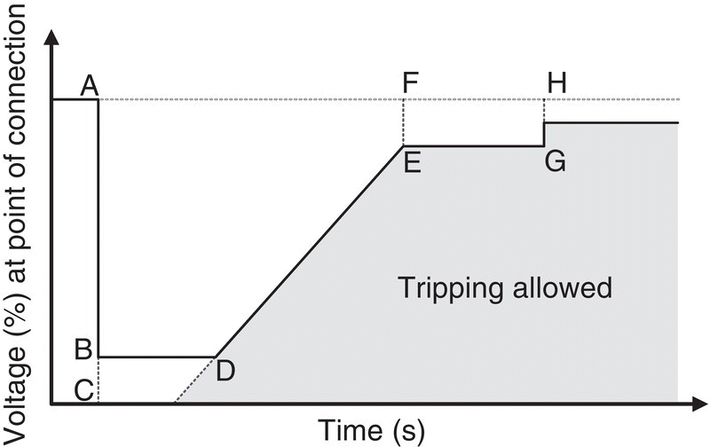
Figure 1.1 Generic FRT voltage versus time characteristic curve.
Table 1.1 FRT voltage and time values for European grid codes.
| Grid Code | BC | BD | AF | FE | AH | HG |
| Denmark | 25% | 0.1 s | 0.75 s | 25% | 10 s | N.A. |
| Germany | 0% | 0.15 s | 0.15 s | 30% | 0.7 s | 10% |
| Ireland | 15% | 0.625 s | 3 s | 10% | N.A. | N.A. |
| Spain | 20% | 0.5 s | 1 s | 20% | 15 s | 5% |
| Spain (Canary Islands) | 0% | 0.5 s | 1 s | 20% | 15 s | 5% |
| United Kingdom | 0% | 0.14 s | 1.2 s | 20% | 2.5 s | 15% |
| Portugal | 20% | 0.5 s | 1.5 s | 20% | 10 s | N.A. |
More recently, interest in large photovoltaic (PV) plants has gaining additional attention. Therefore, specific control requirements for photovoltaic inverters regarding FRT capabilities and voltage control are beginning to become a research topic, which will be developed in the near future[10].
The consequent displacement of synchronous generators affects power system inertia and primary frequency control capabilities, limiting further integration of RES. In order to overcome such limitations, the possibility of endowing wind energy converters with additional control loops in order to provide either inertia emulation capabilities and primary frequency regulation has been discussed[8, 11]. The general approach is to operate RES with a certain reserve margin through the appropriate use of deloading mechanisms. Thus, the reserve margin can be autonomously deployed in case of frequency deviations through the use of a power reference‐frequency droop control.
Additionally, a supplementary control‐loop based on the rate of change of the frequency deviation enables RES to emulate an inertial response. Similar operational characteristics are being envisioned for large offshore wind farms connected to a mainland grid through multiterminal high‐voltage direct current grids[12]. Energy storage systems can also provide an important contribution to primary frequency control, namely, in island systems[13], but also in interconnected systems[14].
ADVANCES IN RENEWABLE ENERGY FORECASTING
During the last 15 years, research work has been conducted on developing forecasting algorithms which achieve a forecast error reduction and an expansion of forecasting products[3]. Furthermore, the number of companies selling forecasting services for RES has proliferated, and the reliability and availability of their service has improved. Presently, SOs use forecasts in their daily operation, embedded in decision‐making processes[15]. Research on wave energy forecasting is also being conducted[16], although this technology is not at the maturity levels of wind and solar technologies.
At a regional/national level, wind power forecasting (WPF) literature reports a normalized mean absolute error (NMAE) of around 6–10% and a normalized root mean square error (NRMSE) of around 8–12% of the installed capacity for 24 hours ahead, rising to 11–14% and 14–17% for 48 hours ahead[3]. For solar power forecasting (SPF), the NRMSE is around 4.3–4.9% for day‐ahead forecasts[17]. The load forecast error is generally measured as a mean absolute percentage error and its value is around 1–2% for 24‐hours ahead forecasts[18]. Note that the real impact of the RES forecast errors can only be measured by an increase in power system operating costs (e.g. increased use of reserves for balancing forecast errors).
Wind Power Forecasting
In general, SOs only need WPFs for a horizon up to 3 days ahead. This time horizon can be divided into two classes[3]: (i) very short term, for a maximum of 6 hours ahead with different time steps (10, 15, 30, and 60 minutes), (ii) short term, for a maximum of 72 hours ahead in 30 and 60 minute time steps. The algorithms used to produce a WPF for these two horizons can differ in type and input data.
Forecasting algorithms for very short‐term horizons use as input past values of the time series. Classic examples are models based on the autoregressive integrated moving average[19], but recently, regime‐switching models[20], such as Markov‐switching autoregressive, are being used for capturing the influence of some complex meteorological variables on the power fluctuations. Furthermore, the combination of dispersed meteorological on‐site and off‐site observations and mesocale numerical weather predictions (NWP)[21] can lead to significant improvements in very‐short‐term horizons[22].
Forecasting algorithms for a short‐term horizon require NWP data. Several statistical and machine learning algorithms have been applied for converting the forecasted meteorological variables into wind power generation forecasts[3]. The use of cost functions for fitting prediction models under non‐Gaussian errors[23], as well as the combination of different statistical and NWP models[24], can improve accuracy.
In addition to research work seeking a forecast error reduction, different forecasting products have been developed: regional forecasts, uncertainty forecasts, and ramp forecasts. These forecasts are inputs to the power system management algorithms reviewed in the following sections.
Regional (or aggregated) forecasts, resulting from a process called upscaling, consists of estimating the total wind power, using information from forecasts of representative wind farms, for which NWP and/or online observations are available[25]. This process is justified when the observations from some wind farms are unavailable or the data quality is poor. From the literature, it is known that the aggregation of wind farms reduces the forecast error because of spatial smoothing effects[26].
A point forecast does not give any information about the errors associated with the forecasted value. This motivated the development of advanced physical and statistical methods for estimating and communicating wind power uncertainty. This uncertainty can have different representations: probabilistic, statistical, and meteorological‐based scenarios.
In the literature, a broad set of statistical methods for producing probabilistic WPF can be found, such as local quantile regression[27] or conditional kernel density estimators[28]. The probabilistic forecasts can be expressed as a set of quantiles or interval forecasts (as depicted in Figure 1.2a), or a probability density function (pdf), or moments from the distribution. However, the forecasts produced by these methods do not include the temporal and spatial dependency of the forecast errors. The dependency of the errors is valuable information for time‐dependent decision‐making problems, such as storage management[29] or UC[30]. The state‐of‐the‐art in WPF represents this time dependency by scenarios that are time/spatial trajectories or random vectors (as depicted in Figure 1.2b).

Figure 1.2 (a) Forecast intervals, centered in the median, and limited by their lower and upper bounds, which are forecasted quantiles. (b) Twenty statistical‐based scenarios with temporal dependency of errors that respect the marginal distribution of the probabilistic forecasts (i.e. plot in (a)).
The scenarios can be statistical or physical based. Statistical‐based scenarios are generated with simulation techniques that sample random vectors using a dependency structure (e.g. covariance matrix) capturing the temporal/spatial dependencies of the forecast errors. Pinson et al.[31] described a method for sampling random vectors from the forecasted marginal cumulative probability functions. The method uses a multivariate Gaussian distribution where the covariance matrix represents the temporal dependency between the forecast errors. This method can also be extended to include spatial dependency[32].
Physical‐based scenarios (or meteorological ensemble) capture two different sources of error: initial conditions and the model (i.e. representation of the dynamics and physics of the atmosphere). These scenarios are obtained with three approaches: (i) different initial conditions or numerical representations of the atmosphere are used in each run of the NWP system[33]; (ii) outputs of different NWP forecast models or from the same NWP model with different parameterizations; (iii) different forecasts made at different times with the same NWP model[34]. These NWP ensembles can be converted to wind power scenarios[35].
Recently proposed, a different type of scenario is associated with spatial fields[36], which are statistically transformed NWP points from a grid covering the wind farm to an equivalent value representing the surface roughness and terrain at a chosen reference point for the wind farm location. Compared with other uncertainty representations, NWP spatial fields capture phase errors in NWP and sampling errors[37].
Finally, although the scenarios already capture ramps and extreme weather events, another forecast product is ramp forecasting[38]. A ramp forecast provides information (point and probabilistic) about the magnitude and timing (i.e. phase error) of future wind power rapid variations. Bossavy et al.[38] used a filtering/thresholding approach for detecting and forecasting ramps using, as input, forecasts produced with meteorological ensembles. The forecast gives the probability of observing a ramp within a set of time intervals. Ferreira et al.[39] presented a different methodology also based on a high‐pass filter and using statistical scenarios as inputs.
Solar Power Forecasting
Although research on WPF has reached a maturity level, research on SPF could be classified as “under development.” In contrast to WPF, SPF requires specific forecast models for the different technologies, such as concentrated photovoltaic and concentrated solar thermal. Nevertheless, current research is more concentrated on the weather forecasting side.
Differently from WPF, pure statistical models with past observations can produce SPF with an acceptable quality for hours/day‐ahead horizons with hourly time steps[40]. The main reason is that the serial dependency presents a strong daily and weekly seasonal pattern. In fact, the daily cycle of solar irradiation is rather easy to predict. Nevertheless, as ‘shown’ by Ahlstrom and Kankiewicz[41] and depicted in Figure 1.3, intrahourly forecasts present a high variability caused by clouds. In fact, clouds are the main cause of short‐term variation, and clouds of different types, speed, and size represent different impacts in solar power generation.
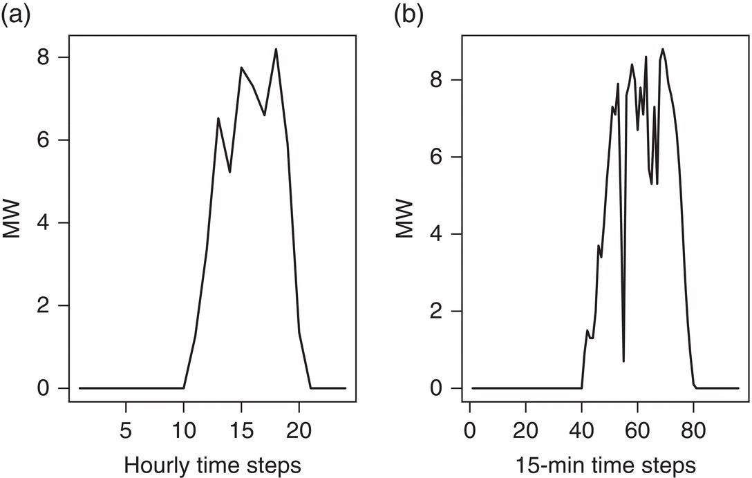
Figure 1.3 Generation variability of solar power due to clouds: (a) hourly average; (b) 15 minute average.
Heinemann et al.[42] identified different input data sources for the various time horizons of interest. For very short‐term horizons (between 30 minutes and 6 hours), the authors suggest the use of satellite‐based cloud motion vector fields. For short‐term horizons (up to 2 days ahead), the forecasts should be based on NWP data.
Heinemann et al.[42] describe very short‐term forecasting algorithms based on cloud‐index images that are predicted with motion vector fields[43] derived from two consecutive images. For short‐term horizons, the authors forecast surface solar irradiance with a NWP mesoscale model. The results showed a good accuracy for clear sky situations, but with broken clouds and overcast conditions, the error increased significantly. A second approach described by the authors is to use a mesoscale NWP model to predict variables describing cloudiness, and this information is converted to solar irradiance. Wittmann et al.[44] examined the importance of combining NWP and aerosol‐based forecasts for day‐ahead horizons. According to the authors, aerosol information is of great relevance for clear sky situations, which are the most frequent situations at solar farm locations.
Lorenz et al.[45] showed that, as with wind farms, the aggregation of photovoltaic (PV) panels and farms decreases the forecast error, by smoothing the cloud effect. A forecast model for a regional forecast is also described[17].
Finally, note that most statistical‐based uncertainty forecasts techniques from WPF can be applied to this problem. Furthermore, meteorological ensembles also have a potential application in SPF.
THE IMPORTANCE OF GENERATION FLEXIBILITY
In the past, flexible power plants were mainly used for handling load variability and uncertainty. RES introduces variability and uncertainty in the supply side, and with a higher magnitude in a scenario with high RES penetration. The wide regional distribution of multiple RES power plants decreases the variability and uncertainty of RES‐based generation[1, 26].
The flexibility of the power plants can be defined as the ability to react (i.e. modify generation levels in response to a command from the SO) quickly enough to rapid generation/load ramps and to deviations between scheduled and realized values. Generation flexibility is characterized by several parameters, such as ramp rate (% of MW per minute), technical and economic minimum generation level, start‐up and shut‐down time. Lannoye et al.[46] propose a methodology to compute the Insufficient Ramping Resource Expectation index, which is a metric that measures power system flexibility for long‐term planning studies.
The following separation between power plants can be made[47]:
- Peak units are able to start, shutdown, or change their generation level very quickly in response to a command from the SO. Units of this type can handle minute‐to‐minute variations and uncertainty, and some examples are open‐cycle gas turbines and hydropower plants.
- Mid‐merit units have the ability to ramp up to their maximum power and down to their minimum, but are slower than the peak units. Examples of these units are combined cycle gas turbines (CCGT) and biomass, and they cover interhour variations and uncertainty.
- Base‐load units have slower response times and normally operate across the entire day or during predefined periods. Units such as coal‐fired plants, nuclear, and geothermal might require around six hours to start or provide a flexible response. These units can provide some flexibility for daily variability.
In addition to these three categories, there are also must‐run units that ensure the dynamic stability of the power system (e.g. minimum online inertia in the system). The minimum generation level of these units may be a critical factor during periods with high penetration of RES.
In some cases, such as France and Germany, nuclear power plants can also provide load‐following capabilities[48]. However, this has economic costs, mainly related with the load factor, as it is only profitable if operating at high load factors (i.e. above 90% of rated power). Furthermore, coal‐ and gas‐fired power plants are becoming more flexible with recent technology. For instance, in Germany, older coal power plants have ramp rates of 2%/minute, whereas new plants have rates of 4–6%/minute[49].
A critical limitation is the minimum load limit of conventional generation units (both technical and economic), which, in general, is around 40–50% of the rated power. Nicolosi[50] reported a lower flexibility in the German power system for the period between October 2008 and December 2009. In situations with generation surplus, all the generation sides together were unable to reduce the generation below 46%, in particular the base‐load technology, which showed high minimum generation levels (due to technical and economic constraints). Soder et al.[51] reported that the Portuguese power system was able to accommodate a very high wind power penetration level (maximum of 81% at 6:45 a.m.) by stopping several hydropower plants between 0 and 4 a.m., and only one gas‐fired plant was kept in operation at 25% of rated power. The flexibility of hydropower units and its pump storage was used to balance wind power fluctuations, and the interconnection with Spain allowed exporting generation surplus.
The cross‐border interconnections also play an important role in increasing the flexibility. It facilitates the use of more flexible power plants where they are needed to balance RES. For example, a high penetration of wind power generation is feasible in Denmark because of the good interconnections with Sweden, Norway, and Germany. The interconnection with Norway provides access to its fast starting hydropower plants, which can be used as reserve capacity contracted in the NordPool electricity market[52]. However, a higher transfer capacity between countries may also create overload problems in situations with high RES‐based generation in one control area[53]. Therefore, cross‐border interconnections should be combined with suitable operational procedures (e.g. forecasting, stochastic power flows) and investment in flexible AC transmission system (FACTS).
The SO can use this flexible generation as reserve capacity, and methods reviewed in the following section optimize the use of this available flexibility.
METHODS FOR HANDLING THE VARIABILITY AND UNCERTAINTY FOR STEADY‐STATE OPERATION
In the operational domain, the SO has a limited time for conducting studies and examining alternatives. The uncertainty in this domain is relatively small when compared with the planning domain, which leads the SO to analyze the current conditions by a series of deterministic methods or rules. The main problem with deterministic approaches is that the user does not know the level of risk associated with future operating conditions. This normally leads to a conservative operation with high operating costs or to unanticipated high risk during operations. As the penetration of renewable generation increases, new management procedures and algorithms emerge for handling generation variability and uncertainty. The use of uncertainty forecasts for renewable generation becomes a relevant input for decision‐aid algorithms. It is important to stress that modeling forecast uncertainty in decision‐making algorithms with the average historical forecast errors (a priori estimation) is not the same as using uncertainty forecasts (a posteriori estimation) directly in the methods, and might lead to conservative and expensive operating strategies.
This section presents an overview of new management algorithms for supporting power system operation in steady‐state conditions with a significant penetration of renewable generation. The majority of the methods in the literature only consider the presence of wind power in the system. Nevertheless, a generalization to other RES (such as solar) is in general possible and straightforward if forecasts for solar power generation are available.
Methods for Setting the Reserve Requirements in the Operational Domain
In each time instant, the SO is responsible for maintaining the balance between generation and load in the power system. This leads to the need for a reserve capacity composed of loads and generation units able to respond to possible problems. Upward and downward reserves are normally necessary. The upward reserve consists of generation units (or loads) online or offline able to, in a short period, increase their generation levels (or decrease their consumption levels). The downward reserve consists of online generation units able to decrease their generation levels or loads able to start consuming (or increase consumption) in a short period.
The classical categories of reserves[54] are: primary (or frequency response), secondary (or regulation reserve), and tertiary (or replacement reserve). Primary reserve is used for stabilizing the system frequency at a stationary value after a disturbance or incident in the time frame of seconds. Secondary reserve is dispatched via automatic generation control for restoring the frequency and interarea power exchanges to their nominal values in a time frame of 15 minutes. The SO restores or supplements secondary reserve levels by manually activating tertiary reserve, in a time frame between 15 minutes and 1 hour.
High penetration levels of renewable energy (mainly wind and solar) in the system require a revision of these reserve categories. Large shares of renewable generation do not create problems (discounting the sudden disconnection due to voltage dips), in interconnected systems, for the timescale of primary reserve[55].
Holttinen et al.[56] divided the reserve categories in: nonevent (normal operation) for variability and forecast errors inside the scheduling period; fast event (contingency operation) for an unplanned outage of a generator or cross‐border transmission line; slow event for expected net‐load ramps; and forecast errors that can occur on longer timescales (tens of minutes to hours). The authors argue that generation from RES does not change fast enough to be a contingency event, and the impact on secondary reserve is lower than the impact on tertiary reserve (both reserves are included in the nonevent category). High penetrations of RES will introduce slow events characterized by high rapid generation ramps and forecast errors.
On the timescale of tertiary reserve, several countries have already created a reserve category for slow events; for example, the manual reserve in Denmark and the balancing reserve in Spain and Hydro‐Quebec.
Deterministic methods (or rules) for setting the reserve requirements have served many SOs in the past[57], mainly because they are easier to be understood and applied by operators, and continued to high security levels with minimum study effort. However, with high levels of renewable generation, excessively conservative approaches would result in a high reserve cost and to a waste of renewable generation‐related benefits. For example, operators not comfortable with the possibility of high forecast errors might define high levels of reserve to compensate potential deviations, thus reducing the economic attractiveness of RES. On the other hand, because risk is not really monitored in deterministic approaches, conservative rules may sometimes fail in specific circumstances not included in their original rationale.
The alternative consists of using probabilistic methods for setting the reserve requirements. In fact, the use of probabilistic methods for setting the reserve in the operating domain is not new. A classic example is the Pennsylvania–New Jersey–Maryland (PJM) interconnection method that evaluates the risk of the committed generation units considering generation outages and load forecast errors[58].
The First Step: Hybrid of Probabilistic–Deterministic Rules
Presently, SOs are starting to include information about forecast errors and uncertainty when defining the reserve requirements. The first step consisted of including a probabilistic component in the former deterministic rules. For example, Electricity Reliability Council of Texas (ERCOT) (Texas Independent SO) defines the nonspinning reserve (the one that handles forecast errors) as the 95th percentile of the observed hourly net load error from the previous 30 days, plus the size of the largest unit[59]. The Spanish SO (REE – Red Eléctrica de España) defines the balancing reserve requirements as the sum of the generation shortage/surplus due to load and wind generation historical forecast errors, and unplanned outages[60]. The European Network of Transmission System Operators for Electricity (ENTSO‐E) revised the rules from the former Union for the Coordination of Transmission of Electricity (UCTE), and a new probabilistic criterion for setting the total reserve (secondary and tertiary) was included[54], but without explicitly mentioning renewable generation.
The Next Step: Probabilistic Methods
Gouveia and Matos[61] extended the PJM method by including the wind power uncertainty modeled with a Markov model. The main limitation (common to other methods) is that the model does not include forecasting information, but only the a priori probability distribution of a set of wind power levels. Thus, the next step is to use probabilistic tools with uncertainty forecasts as input.
The first set of methods assumed that the WPF error follows a normal distribution. Several authors[62, 63] compute the level of imbalance between load and generation by summing the variances of the load and WPF errors (σ2LW = σ2L + σ2W), assuming that both random variables are normal and independent. The reserve requirement needed to deal with the estimated imbalances is given by the variation contained within three standard deviations (3·σLW) of the overall system imbalance. Doherty and O'Malley[64] presented an analytical method for defining the reserve requirements. The model includes generators' unplanned outages (both full and partial outages), load, and WPF errors modeled by a normal distribution. Ortega‐Vazquez and Kirschen[65] described a method for minimizing the sum of expected cost of energy not served (i.e. expected energy not served [EENS] multiplied by the value of lost load) and the operating cost. The wind power and load uncertainties are normal distributions and combined by summing their variances.
However, the normal distribution assumption is highly questionable because the WPF errors' distribution presents high skewness[66] and kurtosis[67], even when several wind farms are aggregated[25]. This assumption, when setting the reserve requirements, may result in a underestimation of the risk[68].
Excluding this normality assumption, Matos and Bessa[69] proposed a probabilistic method that takes as input a probabilistic WPF. The load probabilistic forecast and generation uncertainties (i.e. unplanned outages of conventional generation units and wind turbines plus WPF probabilistic forecast) are convolved with the fast Fourier transform. From the convolution result, risk attributes related with a generation shortage (upward reserve) and surplus (downward reserve) are computed for each reserve level. The results of this exercise are risk/reserve and risk/cost curves for each lead time. As an example, Figure 1.4 depicts the EENS (one of the possible reliability indices) against the reserve level. Establishing this relation allows the SO to make a decision with different methods: (i) set a reference value for the risk and get the reserve level directly from the curve; (ii) establish a trade‐off between reserve cost and risk and find the corresponding optimal reserve level; and (iii) build a value function to find the best compromise between cost and risk. Bessa et al.[70], in the framework of the European project ANEMOS.plus, reported results from an operational demonstration of this method for the Portuguese SO. The demonstration showed that the probabilistic method outperformed the deterministic rules in use at that time.
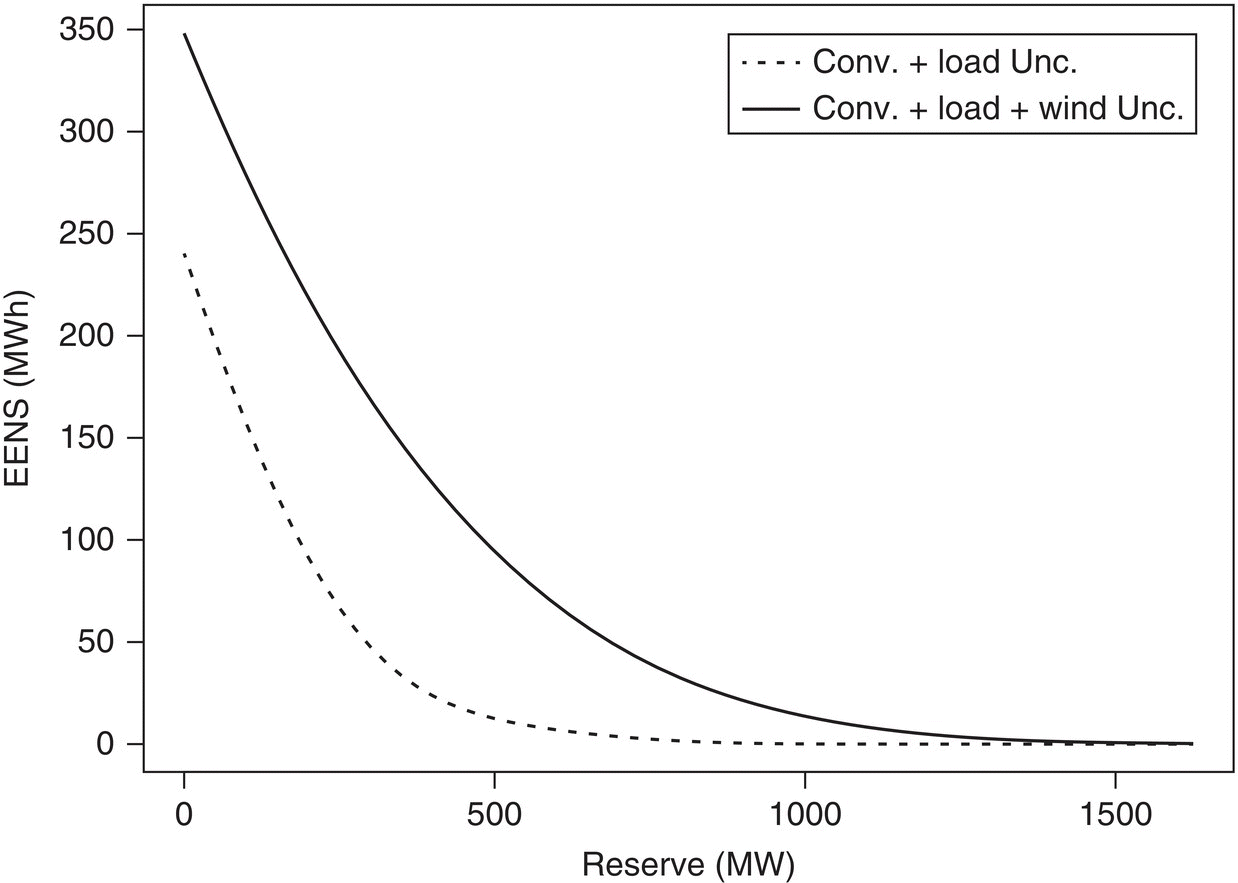
Figure 1.4 Example of the expected energy not supplied as a function of the reserve level for a look‐ahead time and taking into account different sources of uncertainty: conventional and load uncertainty; conventional, load and wind power uncertainty.
Menemenlis et al.[71] describe a method based on convolution which also constructs risk/reserve curves for each lead time. The wind power is modeled with gamma functions fitted with time‐varying parameters for each class of generation level. The decision method consists of establishing a reference value for the risk. The main limitation of the method is that the gamma functions for each wind farm are combined, assuming independence of the uncertainties. This assumption does not consider the spatial dependency of uncertainties, which cannot be neglected. Maurer et al.[72] also proposed a method based on convolution, but the authors did not provide details about how the uncertainties are estimated. An interesting contribution is a two‐step approach for separating the total reserve in secondary and tertiary reserve. The use of ensembles of wind power for setting the reserve was proposed by Pahlow et al.[73] The authors, using ensembles from the multischeme ensemble prediction system[74], compared several rules, such as reserve equal to the difference between the minimum and maximum of the ensemble in each hour. The results showed that the rules based on the ensemble are cost efficient and cover more hours when compared with the deterministic rule (i.e. 11% of installed capacity).
The reviewed methods can be used for purchasing reserve services in a sequential electricity market (i.e. reserve market after the energy market) or included in the UC market clearing process. This second possibility is reviewed in the UC section.
Reserve for Extreme Events
The additional value/information of ramp forecasting in decision‐making problems (e.g. UC) is currently under discussion. Some authors believe that information about ramps should mainly be used as supporting information for the operators, and not as a direct input to an optimization problem (e.g. UC)[39,. A ramp forecast tool can be used to generate alarms to the operator and quantify the risk, supporting preventive measures against rapid variations of wind power.
A particular type of ramp occurs in situations with high wind speed. The wind turbines have a cut‐out wind speed value (generally around 25 m s−1), and above that value the turbine starts to trip. In this case, the SO must deal with an unforeseen rapid drop of wind generation that must be forecasted in order to take preventive measures. Figure 1.5 depicts a wind power reduction of around 600 MW in 1400 MW telemetered by the SO of Portugal, and originated by the cyclone Klaus on 23 January 2009. The forecasting system did not predict this extreme event, and the incident was handled with fast starting hydro units and importing energy from Spain. With solar power generation, an equivalent event can be triggered by fast‐moving clouds.

Figure 1.5 Wind power reduction in Portugal due to extreme wind speed conditions originated by the cyclone Klaus in January 2009 (the wind power generation values are only from telemetered wind farms, available in real time, and not the total wind power generation in Portugal).
Source: Reproduced with permission from Ref. 131. Copyright 2009, REN.
Lin et al.[76] describe a model for estimating the wind power generation reduction under extreme wind conditions. A high‐resolution tool, with calculations in the frequency domain and considering the spatial distribution of the wind farms, simulates power reduction trajectories in a minute‐to‐minute time resolution. From the simulation results, a reserve requirements curve informing how much reserve is required for different wind speed values (close to cut‐out speed) is constructed. In the operational domain, the tool combined with NWP enables the calculation of reduction trajectories samples and a corresponding reserve requirements curve. The main advantage of the described model is that it does not require extensive historical data of the wind farms in the region under analysis.
UC and ED with RES
The UC problem consists of scheduling generation units to minimize the cost of supplying the forecasted load with a set of constraints related to power system security and operation (e.g. ramping rates, start‐up times). The economic dispatch (ED) is based on the UC generation schedule and computes the generation levels of each unit that lead to the lowest possible cost. In summary, the UC decides which units should be running (e.g. on or off) and the ED determines the generation levels of the committed (or online) units. It is common to find these two processes in noninterconnected power systems and in the United States as a market clearing instrument. The UC and ED, in the United States, are used in the following steps[15]: in the day‐ahead market clearing, a security‐constrained UC and ED is used to schedule and dispatch the generation units, using bids (price and quantity pairs in a stepwise increasing function) from market agents; after the day‐ahead market clearing, a reliability assessment commitment (RAC) is performed using security‐constrained UC; a security‐constrained ED is performed in the real‐time market to dispatch the units scheduled by the day‐ahead market and RAC.
Presently, SOs only use deterministic UC/ED, and the load and conventional generation uncertainty is covered in a constraint for guaranteeing a fixed amount of reserve. The state‐of‐the‐art for solving the UC problem is mixed‐integer programming (MIP), which is available in most commercial optimization packages. New UC/ED policies that include probabilistic information can be promising alternatives with increasing levels of RES. For example, ERCOT, when making the day‐ahead plan of the generation resources, uses as a WPF the 20% quantile (i.e. 80% probability of surplus)[77]. This can be understood as a conservative approach that guarantees a safety margin, but increases the cost due to the overcommitment of conventional generation units and leads to a greater need for downward reserve. Thus, an alternative approach is stochastic UC/ED (SUC/SED).
The state‐of‐the‐art for the SUC and SED is a two‐stage stochastic programming with recourse[78]. The UC decisions, excluding fast‐starting generation units, are taken in the first stage (modeled as here‐and‐now variables). The dispatch decisions are made in stage 2, modeled as wait‐and‐see variables, when realized values are known (i.e. real‐time).
Generally, this stochastic problem is converted into a deterministic equivalent that is solved with MIP. The objective function in the published formulations is the minimization of the expected cost[30, 78]. However, subjects such as uncertainty modeling, strategies for including the reserve requirements, and whether or not transmission network constraints are included differ in the literature.
Uncertainty Modeling
Uncertainty is generally modeled through a set of scenarios. However, the characteristics of these scenarios differ from author to author. Some scenarios are generated with techniques that are only suitable for planning studies[79]. For the operational domain, several authors generated scenarios assuming that the wind power follows a normal distribution and without considering the temporal dependency of errors[80–83].
Further UC formulations use different principles. Constantinescu et al.[84] describe a computational framework that combines a NWP model with a sampling technique for generating physical‐based scenarios able to capture the spatial–temporal evolution of forecast errors. Wang et al.[30] and Zhou et al.[85] modeled wind power uncertainty with the method from Pinson et al.[31] Sturt and Strbac[86] use a quantile‐based scenario tree for wind power uncertainty. The scenario tree is constructed from a user‐defined topology, and forecast errors at each node are determined from quantiles of the forecast error distribution.
The use of a large set of scenarios increases the computational requirements. A common practice is to reduce the number of scenarios with a technique that aggregates similar scenarios and eliminates scenarios low probability. The most‐used techniques are backward reduction and forward selection based on a family of Kantorovich or transportation probability metrics[87]. Pappala et al.[82] described a scenario reduction method based on particle swarm optimization, and Sumaili et al.[88] described another algorithm based on clustering techniques.
Modeling the Reserve Requirements
In the SUC, uncertainty is implicitly modeled by using a set of scenarios. According to Bouffard and Galiana[81], the reserves in the SUC are defined internally and there is no need for specifying a priori a reserve requirement. The quantile‐based scenario tree proposed by Sturt and Strbac[86] for modeling wind power uncertainty avoids the need to consider additional reserves for the SUC. Because the scenarios capture the worst‐case tail, it allows the SUC to model dynamic levels of reserve that weigh the cost of providing them compared with the load shedding cost or the cost from committing expensive generation. In the SUC of Morales et al.[89], the reserve requirements are determined considering the value of lost load, electrical energy cost and reserve bids, and also a set of scenarios.
However, other authors also studied the inclusion of a constraint related with reserve requirements, for modeling uncertainty explicitly.
Ruiz et al.[78], although not considering RES uncertainty, showed that the inclusion of a suitable amount of reserve requirements in the SUC formulation resulted in better performance in terms of total cost and unserved energy. Restrepo and Galiana[90] proposed a deterministic UC that includes a constraint that limits the probability of the forecasted residual load exceeding the schedule upward and downward reserve. Wang et al.[30] showed that an SUC with additional reserve for covering the impossibility of comprising all events in a limited set of scenarios performs better than an SUC without additional reserve. Pappala et al.[82] in addition to a set of scenarios, considered additional spinning reserve for dealing with wind power ramps between two consecutive periods.
Stochastic Versus Deterministic UC/ED
Several authors conducted studies comparing deterministic UC and SUC. Tuohy et al.[79] compared both approaches and the SUC decreased the total cost around 0.25%. Interesting differences were: the deterministic UC commits more expensive mid‐merit gas and peaking units; the SUC imports more energy because of the scenarios with low wind power generation; deterministic UC increases the number of startups in the generation units; the SUC presents a better performance in meeting the spinning and replacement reserve requirements.
Wang et al.[30] compared different deterministic and SUC strategies for dealing with wind power uncertainty. Results for a three‐month period showed that a deterministic UC without any WPF (i.e. the wind generation is assumed to be zero) resulted in an overcommitment of conventional units, and when only point forecasts for wind power are included, it leads to the highest cost and load curtailment. The SUC strategies have a relatively low cost, but a deterministic UC with a reserve rule (point forecast minus 10% quantile and 5% of the load) obtained a similar cost. Zhou et al.[85] extended this comparison to the RAC, where fast‐starting units are committed or decommitted by using very‐short‐term wind power probabilistic forecasts and scenarios in the SUC. Both articles show that a dynamic rule for setting the reserve combined with deterministic UC presents a better performance than a fixed reserve value and can yield similar results to SUC, without the need to change considerably the current operational procedures or increasing the computational effort. On other hand, the SUC, as it uses scenarios with temporal correlation, can capture with more detail the ramps between hours and, consequently, compute a suitable reserve for dealing with temporal variability. Another advantage is that it includes the uncertainty impact in the objective function.
Papavasiliou et al.[91] compared an SUC that uses scenarios with a deterministic UC with two alternative rules for setting the reserve: 20% of the forecast peak load, 3% of the forecasted load plus 5% of the forecasted wind power. The SUC improves the daily operational cost over the deterministic UC: 0.39% for the first rule, and 0.54% for the second rule with 7.1% of wind power penetration; 1.33% and 1.09% correspondingly with 14% of wind power penetration.
Lowery and O'Malley[92] studied the impact of WPF errors statistics (i.e. variance, skewness, and kurtosis) on the UC and system operation, using a test system a portfolio from the all Island Grid study (Ireland and Northern Ireland). The authors evaluated which statistical properties of the error distribution contribute to the system operation performance. The results showed that variance has the most impact on the total cost, and skewness only decreases the system cost if complemented by kurtosis. For instance, skewness combined with variance results in an overcommitment of expensive base‐load units due to an incorrect estimation of the tail probabilities. The introduction of these error statistics in the UC changes the generation levels of flexible mid‐merit and peak units, while base‐load units are almost stable. Furthermore, the number of unit startup increases with the forecast uncertainty, with the exception of coal‐based power plants.
The authors also evaluated the impact of over‐ and underestimation of these statistics, and several conclusions were obtained. For example, inaccuracy in kurtosis will aggravate the effects (i.e. system cost) of an underestimation of variance because an overestimation of kurtosis increases the dependency from flexible units, and underestimation overcommits base‐load units. The overestimation of kurtosis when variance is accurate results in a decrease of the total cost because it reduces the use of slower generation units. The lowest number of require startups when variance is underestimated is when skewness is accurate. If variance is overestimated, inaccurate skewness reduce the number of startups of flexible units due to an incorrect estimation of the expected wind power.
Constrained SUC/SED
The constrained UC/ED is particularly important for countries (e.g. United States) with nodal prices. When the transmission network constraints are included, new optimization techniques are needed for solving the problem.
Wu et al.[93] use Lagrangian relaxation to decompose the optimization problem in tractable deterministic constrained SUC subproblems that can be solved with MIP. Wang et al.[80] divided a constrained SUC in a master problem according to the wind power scenario. The security of an initial dispatch is checked in a subproblem, and a redispatch is made for mitigating violations. If the redispatch is insufficient, Benders decomposition is used to revise the generation commitment of the master problem. Morales et al.[89] present a network‐constrained market‐clearing mechanism for energy and reserve (spinning and nonspinning) optimization, considering wind power uncertainty. A two‐stage stochastic programming problem is proposed. The first optimization stage comprises the constraints and rules of the electricity market, whereas the second stage represents the power system operation and physical limitations.
Managing Network Congestion
A “weak” transmission network with a high penetration of RES is prone to congestion situations, which limits the benefits arising from RES integration. For instance, network bottlenecks bind the reduction in operational costs promoted by wind power and increase the amount of curtailed wind generation during low load periods[77, 89]. The use of power flow tools capable of including renewable energy uncertainty can help detect and manage situations with congestion, avoiding curtailment of renewable energy, and in the medium term can defer network investments.
Two approaches can be found for including uncertainty in power flow calculations: probabilistic power flow (PPF) and fuzzy power flow (FPF). Both methods calculate, under steady‐state conditions, the probability distributions or fuzzy values (possibility distributions) for voltages (angle and magnitude), active and reactive power flows, and active losses.
In PPF studies, wind speed uncertainty is frequently modeled by a Weibull distribution[94]. However, this modeling assumption is not suitable for the operational domain because the goal is to include forecast uncertainty. Moreover, the spatial dependency between the random variables is also important for power flow calculations.
The first PPF considering WPF uncertainty was developed by Hatziargyriou et al.[95], for radial distribution networks. The main limitations are the assumption of a normal distribution for the WPF error, and dependencies are neglected. Morales et al.[96] presented a PPF that includes uncertainty through the statistical moments (i.e. mean, variance, skewness, and kurtosis) of the distribution and also includes the spatial dependency of uncertainties. The authors proposed an analytical method based on a modified point‐estimate method (PEM). The dependent input random variables are transformed into independent variables, using an orthogonal transformation. Furthermore, the authors also described a Monte Carlo method for solving the PPF through simulation, using spatial dependent scenarios. The comparison between the two methods showed that the Monte Carlo method takes about 350 times longer than PEM, and with a 95% confidence level, the solutions provided by both methods are the same. Furthermore, it was shown that the dependency between WPF affects more the active power flow, and an increase in the correlation coefficient results in an increase of the power flow standard deviation.
Usaola[97] describes an analytical method for PPF based on the cumulant method and the Cornish‐Fisher expansion series. A small number of convolution operations are conducted for multimodal distributions. The method accepts dependent/independent, continuous/discrete random variables. WPF uncertainty is modeled with beta functions conditioned to the level of injected power, and dependent scenarios are generated with a sampling process similar to others in the literature[31]. The author compared the proposed method with a PEM with independent random variables. The results showed that the PEM attains a good performance (i.e. average error between moments of the power flows) for the independent case up to the second‐order moment, whereas the proposed method behaves better in the dependent case.
Bessa et al.[70] adapted the classical FPF for including WPF uncertainty. A set of forecasted quantiles is converted into a (triangular) fuzzy number. The FPF, in the framework of the ANEMOS.plus project, was operationally demonstrated for the Portuguese SO, and the goal was to detect possible congestions and voltage violations in the market dispatch for the next day. The demonstration showed that in hours where wind power was underforecasted, leading to branch congestion, the deterministic power forecast (PF) was unable to detect congestion, whereas the FPF, depending on the selected cutoff, was capable of detecting possible congestion. Evaluation analysis for the whole demonstration period (six months) showed that deterministic PF has the lowest percentage value of false alarms, but at the same time, has the highest percentage of overlooked congestions. FPF, with a cutoff properly defined by the user, offers a more balanced solution between the percentage of false alarms and the percentage of overlooked congestions.
All reviewed methods were applied only for detecting congestion situations under normal steady‐state operation. Some SOs also run power flow calculations with branch contingencies (N‐1 regime) as the ENTSO‐E Policy 3 suggests[98]. Moreover, the methods do not define (at least directly) any preventive/corrective action or perform a redispatch for solving the problem.
Vlachogiannis[99] proposed a constrained PPF that includes uncertainties from both wind power and electric vehicles (EVs). The method uses a learning algorithm based on learning automata systems for determining the values of continuous and discrete control variables. The goal is to determine robust values for the control variables that maintain the risk of constraints' violation below a predefined level. This method has the following limitations: WPF are not included (i.e. wind speed uncertainty is modeled with a Weibull distribution) and spatial and temporal dependencies are neglected.
An alternative approach is an optimal power flow (OPF). Jabr and Pal[100] described an OPF algorithm that minimizes the generation costs, including a cost term for wind power spilling and another for using reserves due to a wind power shortage. Wind power uncertainty is represented by a probability mass function. However, the main limitation of the method is that uncertainty is only included in the objective function. Capitanescu et al.[101] describes an optimization algorithm for day‐ahead steady‐state security assessment. The algorithm based on power injection scenarios defines preventive and corrective control actions that guarantee power system security for any possible contingency. The algorithm is divided into three stages: day‐ahead decisions; preventive control actions; and correction post‐contingency actions. These stages involve OPF and security constrained OPF. The authors did not consider RES uncertainty explicitly. However, the model can be extended to include this uncertainty source (e.g. using physical or statistical scenarios). The method also presents a high computational time, but parallel computing and scenario reduction techniques can improve the performance.
THE ROLE OF STORAGE DEVICES
Interconnected Power Systems
Storage units such as pumped hydro storage (PHS) or compressed air energy storage (CAES) can play an important role in handling RES variability and uncertainty[102]. Hedegaard and Meibom[103] examined the application of different storage technologies for balancing power at different timescales. The authors analyzed several technologies (i.e. lead‐acid batteries, flow batteries, EVs, CAES, PHS, electrolysis combined with fuel cells) and concluded that all are suitable for intrahour and intraday/day‐ahead balancing. CAES, PHS, and electrolysis combined with fuel cells showed potential for several days ahead and seasonal horizons.
Two different business models can be envisioned for exploring the economic and technical potential of storage devices. The first model consists of having an electrical utility aggregating small or large storage facilities. This utility can combine storage with RES for smoothing forecast errors, and/or price arbitrage (i.e. store in low‐price hours and sell during high‐price hours), and/or participate in the ancillary services market. In the second business model, storage is an asset of the distribution or transmission SO. In this model, storage can be used for balancing services, solving network congestions, voltage support (in the distribution grid), and decreasing operational costs.
In the literature, it is common to find optimization algorithms for coordinating storage units with RES plants[29]. Long‐term evaluations of different storage technologies[104, 105], considering capital costs, show that RES combined with storage can lead to a negative net present value, even when selling reserve services. This economic assessment depends on the price differential between peak and valley hours and reserve prices.
Economics are also important for assessing the value of storage units operated by a SO. Nyamdash et al.[105] show that storage offsets the cost introduced by wind power, as it reduces the participation of mid‐merit units and increases the participation of base‐load units. Nevertheless, this conclusion is only valid for small storage power rating (200–600 MW), as large storage power rating (1200–1800 MW) can shift the load peak to the night period. The authors also evaluated the impact on the net load under different operational strategies. A strategy called mid‐merit (i.e. 12 hours of night charge and 12 hours of day discharge) leads to less wind power curtailment and decreases the net load variability.
Meibom et al.[106] tested an SUC in the Irish power system and showed that there is no general change in the daily operation of pumped hydro units with the increased wind power capacity in the system. This means that storage is mainly driven by load variation. Tuohy and O'Malley[107], using a similar SUC model, studied the operation of the Irish power system with high penetrations of wind power and PHS. The results show that the main advantage offered by PHS is to decrease wind power curtailment, but only at high wind power installed levels. It is also shown that storage provides flexibility for dealing with WPF uncertainty, and the need for storage decreases with the forecast error. Economic analysis (from the SO perspective) also lead to conclusions similar to the abovementioned authors. The main economic savings from storage are from avoiding wind curtailment, but this is only significant for high wind penetration levels (e.g. between 42% and 55%). The authors also show that with increasing wind power, the interconnections are used more for exporting energy, decreasing the need for storage.
Connolly et al.[108] make a similar study and reach similar conclusions, considering the complete energy system (e.g. electricity, transport, and heat) using the EnergyPLAN tool, but without simulating with detail power system operation on an hourly resolution.
Isolated Power Systems
Fast output power variability occurring in timescales less than a minute are likely to induce significant network frequency variations in isolated power systems. The mitigation of such unwanted effects that may lead to system instability can be achieved through the use of energy storage systems that are able to provide high cycling capabilities and high ramp rates as a result of the continuous operation that is required for effective and fast power modulation. Short‐timescale energy storage solutions based on flywheels, supercapacitors, or superconducting magnetic energy storage systems (SMES) are the preeminent technologies for this specific application[55, 102].
The use of supercapacitors in the DC link of the back‐to‐back AC/DC/AC converter of individual doubly fed induction generators (DFIG) in a wind farm is proposed by Qu and Qiao[109] as a way to mitigate global wind farm active power fluctuations resulting from wind variation in very short timescale. Similarly, the use of flywheel storage systems to mitigate wind power fluctuations is presented and discussed by Cimuca et al.[110] The combined use of different energy storage technologies such as flywheels, supercapacitors, or batteries in hybrid systems with offshore wind generation, diesel, and photovoltaic generation is presented by Ray et al.[111] Nomura et al.[112] proposed the use of SMES to smooth the power fluctuations of a 100 MW wind farm. The SMES system is used in a wind farm that is interconnected with a grid through a back‐to‐back DC link. The authors propose a strategy that enables the use of the stored energy in the SMES in order to compensate for the inertia of the turbines, allowing fast wind turbine speed control, depending on the wind condition.
In small islands with low grid inertia, the installation of energy storage solutions can significantly increase system security and planning flexibility for renewable integration, while providing adequate regulation capabilities to fulfill load‐frequency control requirements. The general operation philosophy of an energy storage system in an isolated system is to provide a continuous balance between demand and supply, thus absorbing the excess of power or injecting power into the system. As a result, a significant improvement in global system stability can be achieved, contributing to higher RES penetration levels in isolated power systems. The main objectives of the study consider optimal sizing and management of the batteries, aiming to obtain the maximum economic benefit while providing adequate spinning reserves. Oudalov et al.[113] formulate a numerical optimization problem in order to optimize the economical profitability, taking into account investment and operational costs and the difference between the revenues from availability of frequency control reserve and payments resulting from selling excess energy on the spot market. Lee and Wang[114] developed specific strategies in order to coordinate the control of different energy storage technologies such as batteries and flywheels in a hybrid power system containing wind and solar power generation in order to maintain system frequency in a very tight control band.
ACTIVE AND REACTIVE POWER CONTROL OF RES
As previously mentioned, the increasing integration levels of RES into electric power systems has been inducing SOs to request online control requirements over active and reactive power generation levels in order to maintain system operation within acceptable security levels. The main objective is to assure that RES generators provide additional support for global system operation, providing services for reactive power/voltage control as well as active power control, enabling an appropriate dispatch in case of severe situations such as line overloading. It is important to notice that the flexibility of DFIG and variable speed synchronous generators equipped with a full converter allows implementation of specific controllers for active and reactive power control at the turbine level, in coordination with the wind farm supervisory control system.
Delfino et al.[107] have proposed an advanced control scheme enabling photovoltaic units to independently control their active and reactive power injection to the grid. The effectiveness of the control algorithm has been tested through simulation. The effects of reactive power control on a medium‐voltage (MV) grid have been highlighted, showing benefits in the voltage profile. Turitsyn et al.[108] have investigated the opportunity to control reactive power injection from a PV inverter to promote voltage regulation under stressed transient conditions. The proposed control solution presents an opportunity for distribution utilities to optimize the performance of distribution units and even minimize thermal losses. This control strategy installed at the PV inverter level proposes as future work reactive power control even during night periods when sunshine is not available, allowing the inverter to perform as a FACTS device.
Rodríguez‐Amenedo et al.[115] proposed a hierarchical control architecture headed by a supervisory control system for active and reactive power control at the wind farm substation level in coordination with specific control actions implemented at the turbine level for local control of active and reactive power. The proposed structure allows the wind power to follow a given reference provided by the SO or to follow a strategy of maximization of power production if no reference is provided. Moursi et al.[116] described strategies for secondary voltage control in a remote grid bus through appropriate reactive power management in a wind farm equipped with a DFIG. System parameters such as short‐circuit ratio at the wind farm connection point, as well as communication requirements and inherent delays, are taken into consideration. Additionally, the authors developed a strategy for reactive power allocation to individual wind turbines within the wind farm.
Almeida et al.[117] proposed the development of a wind turbine dispatch strategy in a wind farm following SO requests either for active and/or reactive power. The authors consider that wind turbines are operated on a deloaded maximum power extraction curve and will respond to a supervisory wind farm control after a request from a SO to adjust the outputs of the wind park. The authors also suggest the development of a wind power dispatch center concept, illustrated in Figure 1.6, that will interact with individual wind farms and with the SO to which they are connected in order to implement a concept similar to a virtual power plant that will allow for the global coordination of power injections from different wind farms.

Figure 1.6 Architecture of a wind power dispatch center.
In cases with network congestion, a supervisory control strategy for dynamic redispatching of variable speed wind generators and conventional generators is proposed by Vergnol et al.[118] Under these conditions, grid integration of RES generation is increased while ensuring network security criteria.
MARKET RULES AND PRODUCTS FOR DEALING WITH VARIABILITY AND UNCERTAINTY
Some changes in the market rules and new products can help the SO in managing variability and uncertainty. For example, the participation of RES generation in the electricity market through an intermediary agent or their integration in a portfolio with different generation technologies decreases the forecast error[119, 120].
Another possibility is very‐short‐term trading of RES. This can reduce regulation costs, compared with a day‐ahead horizon, by 30% for a horizon between 6 and 12 hours ahead, and 70% for 2 hours ahead[121]. Several authors tested a rolling‐window approach for SUC, with hourly updates of load and generation forecasts (i.e. simulating intraday trading). Tuohy et al.[79] found that the change in base‐load units is small, the use of mid‐merit gas turbines, and the total number of startups all decrease when the uncertainty decreases. Moreover, the number of hours where reserve requirements are not met increases when changing from an hourly to 6‐hours update. Meibom et al.[106] concluded that the demand for replacement reserve increases with wind power penetration and forecast horizon. An interesting conclusion is that the cost reduction due to perfect forecasts changes with the generation portfolio under study. For instance, the rescheduling cost is high in portfolios with a high share of less‐flexible power plants such as coal‐fired thermal plants or CCGTs.
Weber[122] examined different market designs for facilitating operation with a large share of renewable sources. The most favorable design is based on intraday markets similar to the six voluntary intraday sessions of the Iberian market (Portugal and Spain). According to the author, this provides a good balance between the possibility of adjusting the RES bids by using very short‐term forecasts and sufficient liquidity (which is an essential property for market efficiency).
The pricing system of balancing markets should be revised and harmonized across countries/control areas. Vandezande et al.[123] compared single‐ and double‐price systems for the balancing market. In the former, there is a single price for positive and negative imbalances, whereas in the second, there are asymmetric prices for imbalances. The authors show that the two‐price system encourages trading agents to sell energy according to the lowest imbalance price. For example, if the energy shortage price is lower, the agent can develop a strategy for overestimating its generation. Conversely, the one‐price system encourages the agent to offer its expected (or forecasted) value of generation. Bessa et al.[124] also showed that asymmetric prices create an opportunity for introducing a bias in the WPFs, and that this can lead to over‐ and undercommitment situations. In the United States, the penalization schemes for wind power imbalances are more flexible[120]. For example, the Midwest SOs use an 8% tolerance band, and the California SOs settle imbalances on a monthly basis. In some cases, there are no penalizations for deviation[15].
Some market protocols designed for conventional units may not be appropriate for renewable generation, and can create unfair situations or even windfall profits. Sioshansi and Hurlbut[77] explained how a zonal market in ERCOT system created an incentive for overestimating wind power generation in order to receive a curtailment payment for solving network congestion. This allowed a payment even in situations when the wind was insufficient to meet the scheduled quantity. A nodal pricing system was adopted to avoid this behavior. Weijde and Hobbs[125] have shown that nodal prices can decrease startup and variable generation costs, resulting from full modeling of the transmission network (in contrast to approaches based on net transfer capacity). Furthermore, the authors also showed that the coordination of international balancing markets could lower the costs of UC and ED.
EMERGENT APPROACHES
Across the world, different initiatives with a strong involvement of the distribution system operator (DSO) aim to identify solutions toward the implementation of the smart grid concept[126]. Smart Grids provide additional capabilities for the observability and controllability at the distribution network level (e.g. distributed storage, distributed generation, microgeneration, controllable loads). The implementation of a smart grid concept is strongly supported by Information and Communications Technology (ICT), and its synergy with power system engineering enables new features, such as self‐healing and islanding operation, which improve system resilience in the presence of distributed RES generation.
This smart grid concept creates conditions for demand management[127], either by sending direct control signals to the load or sending price signals to induce a certain reaction from the load. This changes the paradigm, moving it from “generation following load” to “load following generation.” The controllable loads can participate (or bid) in reserve markets primarily designed to solve RES forecast errors and ramps. In fact, with increased wind power penetration, a flexible load such as a domestic heat pump can offer similar savings than a PHS, and is less sensitive to changes in fuel prices, interest rates, and the level of storage needs[108, 128].
A very flexible load for demand dispatch is the EV. An EV operating in vehicle‐to‐grid mode (V2G, i.e. bidirectional power injection) can play the same role as storage devices[129], but acting just as a controllable load (i.e. unidirectional controllable injection) can also provide reserve services[127, 129] that can be used for mitigating forecast errors and rapid ramps. Furthermore, an EV with a proper electronic interface control can provide primary frequency control in isolated and micro‐grid systems, allowing the integration of additional wind power without harming power system dynamic security[129].
The smart grid concept is also being transferred to the transmission network and power system operation[130]. The idea consists of developing smart dispatch centers with new functions for monitoring, analyzing, and controlling the power system. These new functions will use, for example, the monitoring capability of phasor measurement units, online algorithms for voltage and small‐signal stability analysis, and algorithms capable of estimating a snapshot of the system operating conditions for the next minutes/hour. Technological advances, such as FACTS, HVDC, and the smart substation concept, complement the new software functions.
CONCLUSIONS
Handling RES (mainly wind and solar power) variability and uncertainty in power system operation can be achieved through forecasting and management tools, and technological advances. Current forecasting algorithms offer an acceptable forecast error, and provide different approaches for modeling uncertainty. Uncertainty forecasts are an important input for stochastic management tools designed for several problems, such as setting the reserve requirements or the UC, that allow an accurate characterization of the risk associated with different decisions. Technological advances in storage devices and the possibility of controlling active/reactive generation of RES power plants offer more flexibility from RES generation.
A relevant issue is that the additional value of new management methods depends upon the characteristics of the power system under analysis. These characteristics are minimum generation levels, transmission and interconnections capacity, wind power penetration, maximum ramping, start‐up times, market gate closure, and so on. For example, a system with a high capacity of fast‐starting units (e.g. hydropower plants) has lower requirements for ramp forecasting algorithms or specific reserve for ramping events, and the impact on the reliability of generation variability is low. In a power system with a long period between day‐ahead scheduling and the operating day, and without intraday scheduling (or trading), good forecasts will be more valued.
In interconnected systems, storage units should be used when the level of curtailed RES becomes significant in the power system. Nevertheless, this will depend on the generation portfolio, interconnection capacity, renewable energy forecast errors and variability. A “good” forecast[124] combined with suitable operational procedures (e.g. stochastic optimization, intraday markets) can avoid the need to invest in storage units. In isolated systems, the use of storage for timescales less than a minute is essential when the penetration levels of renewable generation are high.
The adoption of probabilistic approaches for setting the reserve requirements and UC represent a radical departure from established procedures. Research concerning these methods provides important insights that could be used to improve the deterministic processes or to a full transition to stochastic methods.
Finally, the electricity market role cannot be neglected, and the development of the smart grid paradigm should lead to new market rules capable of extracting the full potential of the new resources (i.e. renewable generation, active loads, and storage units).
ACKNOWLEDGMENTS
This work is funded in part by the ERDF – European Regional Development Fund through the COMPETE Programme (operational programme for competitiveness) and by national funds through the FCT – Fundação para a Ciência e a Tecnologia (Portuguese Foundation for Science and Technology) within project ≪FCOMP – 01–0124‐FEDER‐022701≫.
Ricardo J. Bessa and Bernardo Silva want to express their gratitude to FCT for supporting this work under PhD Scholarships SFRH/BD/33738/2009 and SFRH/BD/61600/2009, cofunded by the European Social Fund through the POPH program.
The authors graciously thank the partners from the European projects ANEMOS.plus (contract no. 038692) and TWENTIES (contract no. 249812) funded in part by the European Commission under the sixth and seventh RTD Framework Programme.
REFERENCES
- 1. Holttinen, H. (2012). Wind integration: experience, issues, and challenges. WIREs Energy Environ. 1: 243–255.
- 2. Abbad, J.R. (2010). Electricity market participation of wind farms: the success story of the Spanish pragmatism. Energy Policy 38: 3174–3179.
- 3. Monteiro C, Bessa R, Miranda V, et al. Wind power forecasting: state‐of‐the‐art 2009. Argonne National Laboratory Report ANL/DIS‐10‐1, 2009. Available at: http://www.dis.anl.gov/pubs/65613.pdf. (Accessed January 2013).
- 4. Ela, E. and O'Malley, M. (2012). Studying the variability and uncertainty impacts of variable generation at multiple timescales. IEEE Trans. Power Syst. 27: 1324–1333.
- 5. Lalor, G., Mullane, A., and O'Malley, M. (2005). Frequency control and wind turbine technologies. IEEE Trans. Power Syst. 20: 1905–1913.
- 6. Mohseni, M. and Islam, S.M. (2012). Review of international grid codes for wind power integration: diversity, technology and a case for global standard. Renewable Sustainable Energy Rev. 16: 3876–3890.
- 7. Carrasco, J.M., Franquelo, L.G., Bialasiewicz, J.T. et al. (2006). Power‐electronic systems for the grid integration of renewable energy sources: a survey. IEEE Trans. Ind. Electron. 53: 1002–1016.
- 8. de Almeida, R.G. and Lopes, J.A.P. (2007). Participation of doubly fed induction wind generators in system frequency regulation. IEEE Trans. Power Syst. 22: 944–950.
- 9. Tsili, M. and Papathanassiou, S. (2009). A review of grid code technical requirements for wind farms. IET Renew. Power Gener. 3: 308–332.
- 10. Alatrash H, Mensah A, Mark E, et al. Generator emulation controls for photovoltaic inverters. In IEEE 8th International Conference on Power Electronics and ECCE Asia (ICPE & ECCE). Korea: The Shilla Jeju; August 30‐September 1, 2011.
- 11. Ramtharan, G., Ekanayake, J.B., and Jenkins, N. (2007). Frequency support from doubly fed induction generator wind turbines. IET Renew. Power Gener. 1: 3–9.
- 12. Silva, B., Moreira, C.L., Seca, L. et al. (2012). Provision of inertial and Sprimary frequency control services using offshore multiterminal HVDC networks. IEEE Trans. Sustainable Energy 3: 800–808.
- 13. Kottick, D., Blau, M., and Edelstein, D. (1993). Battery energy storage for frequency regulation in an island power system. IEEE Trans. Energy Convers. 8: 455–459.
- 14. Aditya, S.K. and Das, D. (2001). Battery energy storage for load frequency control of an interconnected power system. Electr. Power Syst. Res. 58: 179–185.
- 15. Botterud, A., Wang, J., Miranda, V. et al. (2010). Wind power forecasting in U.S. electricity markets. Electr. J. 23: 1040–6190.
- 16. Reikard, G., Pinson, P., and Bidlot, J.‐R. (2011). Forecasting ocean wave energy: the ECMWF wave model and time series methods. Ocean Eng. 38: 1089–1099.
- 17. Lorenz, E., Scheidsteger, T., Hurka, J. et al. (2011). Regional PV power prediction for improved grid integration. Prog. Photovoltaics Res. Appl. 19: 757–771.
- 18. Taylor, J.W. and McSharry, P.E. (2007). Short‐term load forecasting methods: an evaluation based on European data. IEEE Trans. Power Syst. 22: 2213–2219.
- 19. Contaxis, G.C. and Kabouris, J. (1991). Short term scheduling in a wind/diesel autonomous energy system. IEEE Trans. Power Syst. 6: 1161–1167.
- 20. Pinson, P. and Madsen, H. (2012). Adaptive modelling and forecasting of offshore wind power fluctuations with Markov‐switching autoregressive models. J. Forecasting 31: 281–313.
- 21. Giebel G, Badger J, Louka P, et al. Description of NWP, mesoscale and CFD models. Deliverable 4.1, EU Project ANEMOS; 2006. Available at: http://130.226.56.153/zephyr/publ/ANEMOS_D4.1_ModelDescription.pdf. (Accessed January 2013).
- 22. Larson, K.A. and Westrick, K. (2006). Short‐term wind forecasting using off‐site observations. Wind Energy 9: 55–62.
- 23. Bessa, R.J., Miranda, V., and Gama, J. (2009). Entropy and correntropy against minimum square error in offline and online three‐day ahead wind power forecasting. IEEE Trans. Power Syst. 24: 1657–1666.
- 24. Thordarson, F.Ö., Madsen, H., Nielsen, H.A. et al. (2010). Conditional weighted combination of wind power forecasts. Wind Energy 13: 751–763.
- 25. Siebert N. Development of methods for regional wind power forecasting. PhD Thesis. Centre Energétique et Procédés, Mines ParisTech; 2008.
- 26. Focken, U., Lange, M., Mönnich, K. et al. (2002). Short‐term prediction of the aggregated power output of wind farms—a statistical analysis of the reduction of the prediction error by spatial smoothing effects. J. Wind Eng. Ind. Aerodyn. 90: 231–246.
- 27. Bremnes, J.B. (2004). Probabilistic wind power forecasts using local quantile regression. Wind Energy 7: 47–54.
- 28. Bessa, R.J., Miranda, V., Botterud, A. et al. (2012). Time‐adaptive quantile‐copula for wind power probabilistic forecasting. Renewable Energy 40: 29–39.
- 29. Castronuovo, E.D. and Lopes, J.A.P. (2004). On the optimization of the daily operation of a wind‐hydro power plant. IEEE Trans. Power Syst. 19: 1599–1606.
- 30. Wang, J., Botterud, A., Bessa, R. et al. (2011). Wind power forecasting uncertainty and unit commitment. Appl. Energy 88: 4014–4023.
- 31. Pinson, P., Papaefthymiou, G., Klockl, B. et al. (2009). From probabilistic forecasts to statistical scenarios of short‐term wind power production. Wind Energy 12: 51–62.
- 32. Papaefthymiou G, Pinson P. Modeling of spatial dependence in wind power forecast uncertainty. In PMAPS 2008: 10th International Conference on Probabilistic Methods Applied to Power Systems. IEEE: Puerto Rico; May 25–29, 2008.
- 33. Leutbecher, M. and Palmer, T.N. (2008). Ensemble forecasting. J. Comput. Phys. 227: 3515–3539.
- 34. Ziehmann, C. (2000). Comparison of a single‐model EPS with a multi‐model ensemble consisting of a few operational models. Tellus Ser. A 52: 280–299.
- 35. Nielsen HA, Madsen H, Nielsen TS, et al. Wind power ensemble forecasting using wind speed and direction ensembles from ECMWF or NCEP. Denmark Project PSO, Technical Report, 2005. Available at: http://www.risoe.dtu.dk/rispubl/NEI/nei‐dk‐4552.pdf. (Accessed January 2013).
- 36. Cutler, N.J., Outhred, H.R., MacGill, I.F. et al. (2008). Characterizing future large, rapid changes in aggregated wind power using numerical weather prediction spatial fields. Wind Energy 12: 542–555.
- 37. Cutler, N.J., Outhred, H.R., MacGill, I.F. et al. (2012). Predicting and presenting plausible future scenarios of wind power production from numerical weather prediction systems: a qualitative ex ante evaluation for decision making. Wind Energy 15: 473–488.
- 38. Bossavy, A., Girard, R., and Kariniotakis, G. (2013). Forecasting ramps of wind power production with numerical weather prediction ensembles. Wind Energy 16: 51–63.
- 39. Ferreira C, Gama J, Miranda V, et al. Probabilistic ramp detection and forecasting for wind power prediction. In PMAPS 2012—International Conference on Probabilistic Methods Applied to Power Systems. IEEE: Istanbul, Turkey; June 10–14, 2012.
- 40. Mellit, A. and Pavan, A.M. (2010). A 24‐h forecast of solar irradiance using artificial neural network: application for performance prediction of a grid‐connected PV plant at Trieste, Italy. Sol. Energy 84: 807–821.
- 41. Ahlstrom M, Kankiewicz A. Solar power forecasting. In Solar Power: Making High Penetration Possible Workshop. Iowa: Cedar Rapids; October 15, 2010.
- 42. Heinemann, D., Lorenz, E., and Girodo, M. (2006). Forecasting of solar radiation. In: Solar Energy Resource Management for Electricity Generation from Local Level to Global Scale (ed. E.D. Dunlop, L. Wald and M. Suri), 83–94. New York: Nova Science Publishers Inc.
- 43. Bannehr, L., Rohn, M., and Warnecke, G. (1996). A functional analytic method to derive displacement vector fields from satellite image sequences. Int. J. Remote Sens. 17: 383–392.
- 44. Wittmann, M., Breitkreuz, H., Schroedter‐Homscheidt, M. et al. (2008). Case studies on the use of solar irradiance forecast for optimized operation strategies of solar thermal power plants. IEEE J. Sel. Top. Appl. Earth Obs. Remote Sens. 1: 18–27.
- 45. Lorenz, E., Hurka, J., Heinemann, D. et al. (2009). Irradiance forecasting for the power prediction of grid‐connected photovoltaic systems. IEEE J. Spec. Top Earth Obs. Remote Sens. 2: 2–10.
- 46. Lannoye, E., Flynn, D., and O'Malley, M. (2012). Evaluation of power system flexibility. IEEE Trans. Power Syst. 27: 922–931.
- 47. Harnessing Variable Renewables – A Guide to the Balancing Challenge . Paris, France: OECD/IEA; 2011.
- 48. Lokhov A. Technical and economic aspects of load following with nuclear power plants. Nuclear Energy Agency; 2011. Available at: http://www.oecd‐nea.org/ndd/reports/2011/load‐following‐npp.pdf. (Accessed January 2013).
- 49. Auer J, Keil J. State‐of‐the‐art electricity storage systems. Deutsche Bank Research, 2012. Available at: http://www.dbresearch.com/PROD/DBR_INTERNET_EN‐PROD/PROD0000000000286166/State‐of‐the‐art+electricity+storage+systems%3A+Indispensable+elements+of+the+energy+revolution.PDF. (Accessed January 2013).
- 50. Nicolosi, M. (2010). Wind power integration and power system flexibility—an empirical analysis of extreme events in Germany under the new negative price regime. Energy Policy 38: 7257–7268.
- 51. Soder, L., Abildgaard, H., Estanqueiro, A. et al. (2012). Experience and challenges with short‐term balancing in European systems with large share of wind power. IEEE Trans. Sustainable Energy 3: 853–861.
- 52. Gül T, Stenzel T. Variability of wind power and other renewables—management options strategies. International Energy Agency Report, 2005. Available at: http://www.uwig.org/IEA_Report_on_variability.pdf. (Accessed January 2013).
- 53. European wind integration study (EWIS) towards a successful integration of wind power into European electricity grids. Phase I Final Report; 2007. Available at: http://www.wind‐integration.eu/downloads/library/EWIS_Final_Report.pdf. (Accessed January 2013).
- 54. ENTSO‐E. Operating Handbook—Policies P1: Load‐Frequency Control and Performance ; 2009. Available at: https://www.entsoe.eu/publications/system ‐ operations ‐ reports / operation ‐ handbook/. (Accessed January 2013).
- 55. Banakar, H., Luo, C., and Ooi, B.T. (2008). Impacts of wind power minute‐to‐minute variations on power system operation. IEEE Trans. Power Syst. 23: 150–160.
- 56. Holttinen, H., Milligan, M., Ela, E. et al. (2012). Methodologies to determine operating reserves due to increased wind power. IEEE Trans. Sustainable Energy 3: 713–723.
- 57. Rebours Y. A comprehensive assessment of markets for frequency and voltage control ancillary services. PhD Thesis. University of Manchester, Faculty of Engineering and Physical Sciences; 2008.
- 58. Anstine, L.T., Burke, R.E., Casey, J.E. et al. (1963). Application of probability methods to the determination of spinning reserve requirements for the Pennsylvania–New Jersey–Maryland interconnection. IEEE Trans. Power Apparatus Syst. 82: 720–735.
- 59. ERCOT. ERCOT methodologies for determining ancillary service requirements; 2011.
- 60. Secretaría General de Energía. REE P.O. 1.5—Establecimiento de la reserva para la regulación frecuencia‐potencia. BOE núm. 2006, 173:27473–27474.
- 61. Gouveia, E. and Matos, M.A. (2009). Evaluating operational risk in a power system with a large amount of wind power. Electr. Power Syst. Res. 79: 734–739.
- 62. Soder, L. (1993). Reserve margin planning in a wind‐hydrothermal power system. IEEE Trans. Power Syst. 8: 564–571.
- 63. Holttinen, H. (2005). Impact of hourly wind power variations on the system operation in the Nordic countries. Wind Energy 8: 197–218.
- 64. Doherty, R. and O'Malley, M. (2005). New approach to quantify reserve demand in systems with significant installed wind capacity. IEEE Trans. Power Syst. 20: 587–595.
- 65. Ortega‐Vazquez, M.A. and Kirschen, D.S. (2009). Estimating the spinning reserve requirements in systems with significant wind power generation penetration. IEEE Trans. Power Syst. 24: 114–124.
- 66. Lange, M. (2005). On the uncertainty of wind power predictions—analysis of the forecast accuracy and statistical distribution of errors. J. Sol. Energy Eng. 127: 177–194.
- 67. Bludszuweit, H., Dominguez‐Navarro, J.A., and Llombart, A. (2008). Statistical analysis of wind power forecast error. IEEE Trans. Power Syst. 23: 983–991.
- 68. Bessa RJ, Matos MA. Comparison of probabilistic and deterministic approaches for setting operating reserve in systems with high penetration of wind power. In 7th Mediterranean Conference and Exhibition on Power Generation, Transmission, Distribution and Energy Conversion (Medpower). Agia Napa: Cyprus; November 7–10, 2010.
- 69. Matos, M.A. and Bessa, R.J. (2011). Setting the operating reserve using probabilistic wind power forecasts. IEEE Trans. Power Syst. 26: 594–603.
- 70. Bessa, R.J., Matos, M.A., Costa, I.C. et al. (2012). Reserve setting and steady‐state security assessment using wind power uncertainty forecast: a case study. IEEE Trans. Sustainable Energy 3: 827–836.
- 71. Menemenlis, N., Huneault, M., and Robitaille, A. (2012). Computation of dynamic operating balancing reserve for wind power integration for the time‐horizon 1–48 hours. IEEE Trans. Sustainable Energy 3: 692–702.
- 72. Maurer, C., Krahl, S., and Weber, H. (2009). Dimensioning of secondary and tertiary control reserve by probabilistic methods. Eur. Trans. Electr. Power 19: 544–552.
- 73. Pahlow, M., Möhrlen, C., and Jørgensen, J.U. (2009). Application of cost functions for large scale integration of wind power using a multi‐scheme ensemble prediction technique. In: Optimization Advances in Electric Power Systems (ed. E.D. Castronuovo). New York: Nova Science Publishers Inc.
- 74. Lang S, Möhrlen J, Jørgensen J, et al. Application of a multi‐scheme ensemble prediction system for wind power forecasting in Ireland and comparison with validation results from Denmark and Germany. In European Wind Energy Conference EWEC'06. Athens, Greece; February 27‐March 2, 2006.
- 75. Otterson S, Pinson P. Are ramp forecasts really useful? In EWEA Annual Event. Copenhagen, Denmark; April 16–19, 2012.
- 76. Lin, J., Sun, Y.‐Z., Cheng, L. et al. (2012). Assessment of the power reduction of wind farms under extreme wind condition by a high resolution simulation model. Appl. Energy 96: 21–32.
- 77. Sioshansi, R. and Hurlbut, D. (2010). Market protocols in ERCOT and their effect on wind generation. Energy Policy 38: 3192–3197.
- 78. Ruiz, P.A., Philbrick, C.R., Zak, E. et al. (2009). Uncertainty management in the unit commitment problem. IEEE Trans. Power Syst. 24: 642–651.
- 79. Tuohy, A., Meibom, P., Denny, E. et al. (2009). Unit commitment for systems with significant wind penetration. IEEE Trans. Power Syst. 24: 592–601.
- 80. Wang, J., Shahidehpour, M., and Li, Z. (2008). Security‐constrained unit commitment with volatile wind power generation. IEEE Trans. Power Syst. 23: 1319–1327.
- 81. Bouffard, F. and Galiana, F.D. (2008). Stochastic security for operations planning with significant wind power generation. IEEE Trans. Power Syst. 23: 306–316.
- 82. Pappala, V.S., Erlich, I., Rohrig, K. et al. (2009). Stochastic model for the optimal operation of a wind‐thermal power system. IEEE Trans. Power Syst. 24: 940–950.
- 83. Xiao, J., Hodge, B.‐M.S., Pekny, J.F. et al. (2011). Operating reserve policies with high wind power penetration. Comput. Chem. Eng. 35: 1876–1885.
- 84. Constantinescu, E.M., Zavala, V.M., Rocklin, M. et al. (2011). A computational framework for uncertainty quantification and stochastic optimization in unit commitment with wind power generation. IEEE Trans. Power Syst. 26: 431–441.
- 85. Zhou, Z., Botterud, A., Wang, J. et al. (2012). Application of probabilistic wind power forecasting in electricity markets. Wind Energy.
- 86. Sturt, A. and Strbac, G. (2012). Efficient stochastic scheduling for simulation of wind‐integrated power systems. IEEE Trans. Power Syst. 27: 323–334.
- 87. Growe‐Kuska N, Heitsch H, Romisch W. Scenario reduction and scenario tree construction for power management problems. In IEEE Bologna PowerTech Conference. Bologna, Italy; June 23–26, 2003.
- 88. Sumaili J, Keko H, Miranda V, et al. Finding representative wind power scenarios and their probabilities for stochastic models. In ISAP 2011 – 16th International Conference on Intelligent System Applications to Power Systems. Hersonissos, Greece; September 25–28, 2011.
- 89. Morales, J.M., Conejo, A.J., and Pérez‐Ruiz, J. (2009). Economic valuation of reserves in power systems with high penetration of wind power. IEEE Trans. Power Syst. 24: 900–910.
- 90. Restrepo, J.F. and Galiana, F.D. (2011). Assessing the yearly impact of wind power through a new hybrid deterministic/stochastic unit commitment. IEEE Trans. Power Syst. 26: 401–410.
- 91. Papavasiliou, A., Oren, S.S., and O'Neill, R.P. (2011). Reserve requirements for wind power integration: a scenario‐based stochastic programming framework. IEEE Trans. Power Syst. 26: 2197–2206.
- 92. Lowery, C. and O'Malley, M. (2012). Impact of wind forecast error statistics upon unit commitment. IEEE Trans. Sustainable Energy 3: 760–768.
- 93. Wu, L., Shahidehpour, M., and Li, T. (2007). Stochastic security‐constrained unit commitment. IEEE Trans. Power Syst. 22: 800–811.
- 94. Villanueva, D., Pazos, J.L., and Feijóo, A. (2011). Probabilistic load flow including wind power generation. IEEE Trans. Power Syst. 26: 1659–1667.
- 95. Hatziargyriou, N.D., Karakatsanis, T.S., and Papadopoulos, M. (1993). Probabilistic load flow in distribution systems containing dispersed wind power generation. IEEE Trans. Power Syst. 8: 159–165.
- 96. Morales, J.M., Baringo, L., Conejo, A.J. et al. (2010). Probabilistic power flow with correlated wind sources. IET Gener. Transm. Distrib. 4: 641–651.
- 97. Usaola, J. (2009). Probabilistic load flow in systems with wind generation. IET Gener. Transm. Distrib. 3: 1031–1041.
- 98. ENTSO‐E. Operating Handbook – Policy 3: Operational Security; 2009. Available at: https://www.entsoe.eu/publications/system‐operations‐reports/operation‐handbook/. (Accessed January 2013).
- 99. Vlachogiannis, J.G. (2009). Probabilistic constrained load flow considering integration of wind power generation and electric vehicles. IEEE Trans. Power Syst. 24: 1808–1817.
- 100. Jabr, R.A. and Pal, B.C. (2009). Intermittent wind generation in optimal power flow dispatching. IET Gener. Transm. Distrib. 3: 66–74.
- 101. Capitanescu, F., Fliscounakis, S., Panciatici, P. et al. (2012). Cautious operation planning under uncertainties. IEEE Trans. Power Syst. 27: 1859–1869.
- 102. Díaz‐González, F., Sumper, A., Gomis‐Bellmunt, O. et al. (2012). A review of energy storage technologies for wind power applications. Renewable Sustainable Energy Rev. 16: 2154–2171.
- 103. Hedegaard, K. and Meibom, P. (2012). Wind power impacts and electricity storage—a time scale perspective. Renewable Energy 37: 318–324.
- 104. Loisel, R., Mercier, A., Gatzen, C. et al. (2011). Market evaluation of hybrid wind‐storage power systems in case of balancing responsibilities. Renewable Sustainable Energy Rev. 15: 5003–5012.
- 105. Nyamdash, B., Denny, E., and O'Malley, M. (2010). The viability of balancing wind generation with large scale energy storage. Energy Policy 38: 7200–7208.
- 106. Meibom, P., Barth, R., Hasche, B. et al. (2011). Stochastic optimization model to study the operational impacts of high wind penetrations in Ireland. IEEE Trans. Power Syst. 26: 1367–1379.
- 107. Tuohy, A. and O'Malley, M. (2011). Pumped storage in systems with very high wind penetration. Energy Policy 39: 1965–1974.
- 108. Connolly, D., Lund, H., Mathiesen, B.V. et al. (2012). The technical and economic implications of integrating fluctuating renewable energy using energy storage. Renewable Energy 43: 47–60.
- 109. Qu, L. and Qiao, W. (2011). Constant power control of DFIG wind turbines with supercapacitor energy storage. IEEE Trans. Ind. Appl. 47: 359–367.
- 110. Cimuca, G.O., Saudemont, C., Robyns, B. et al. (2006). Control and performance evaluation of a flywheel energy‐storage system associated to a variable‐speed wind generator. IEEE Trans. Ind. Electron. 53: 1074–1085.
- 111. Ray, P.K., Mohanty, S.R., and Kishor, N. (2011). Proportional–integral controller based small‐signal analysis of hybrid distributed generation systems. Energy Convers. Manage. 52: 1943–1954.
- 112. Nomura, S., Ohata, Y., Hagita, T. et al. (2005). Wind farms linked by SMES systems. IEEE Trans. Appl. Supercond. 15: 1951–1954.
- 113. Oudalov, A., Chartouni, D., and Ohler, C. (2007). Optimizing a battery energy storage system for primary frequency control. IEEE Trans. Power Syst. 22: 1259–1266.
- 114. Lee, D.‐J. and Wang, L. (2008). Small‐signal stability analysis of an autonomous hybrid renewable energy power generation/energy storage system part I: time‐domain simulations. IEEE Trans. Energy Convers. 23: 311–320.
- 115. Rodríguez‐Amenedo, J.L., Arnalte, S., and Burgos, J.C. (2002). Automatic generation control of a wind farm with variable speed wind turbines. IEEE Trans. Energy Convers. 17: 279–284.
- 116. Moursi, M.E., Joos, G., and Abbey, C. (2008). A secondary voltage control strategy for transmission level interconnection of wind generation. IEEE Trans. Power Electron. 23: 1178–1190.
- 117. de Almeida, R.G., Castronuovo, E.D., and Lopes, J.A.P. (2006). Optimum generation control in wind parks when carrying out system operator requests. IEEE Trans. Power Syst. 21: 718–725.
- 118. Vergnol, A., Sprooten, J., Robyns, B. et al. (2011). Line overload alleviation through corrective control in presence of wind energy. Electr. Power Syst. Res. 81: 1583–1591.
- 119. Ummels, B.C., Gibescu, M., Kling, W.L. et al. (2006). Integration of wind power in the liberalized Dutch electricity market. Wind Energy 9: 579–590.
- 120. Aparicio, N., MacGill, I., Rivier Abbad, J. et al. (2012). Comparison of wind energy support policy and electricity market design in Europe, the United States, and Australia. IEEE Trans. Sustainable Energy 3: 809–818.
- 121. Holttinen, H. (2005). Optimal electricity market for wind power. Energy Policy 33: 2052–2063.
- 122. Weber, C. (2010). Adequate intraday market design to enable the integration of wind energy into the European power systems. Energy Policy 38: 3155–3163.
- 123. Vandezande, L., Meeus, L., Belmans, R. et al. (2010). Well‐functioning balancing markets: a prerequisite for wind power integration. Energy Policy 38: 3146–3154.
- 124. Bessa, R.J., Miranda, V., Botterud, A. et al. (2011). ‘Good’ or ‘bad’ wind power forecasts: a relative concept. Wind Energy 14: 625–636.
- 125. Weijde, A.H. and Hobbs, B.F. (2011). Locational‐based coupling of electricity markets: benefits from coordinating unit commitment and balancing markets. J. Regul. Econ. 39: 223–251.
- 126. Farhangi, H. (2010). The path of the smart grid. IEEE Power Energ. Mag. 8: 18–28.
- 127. Brooks, A., Lu, E., Reicher, D. et al. (2010). Demand dispatch. IEEE Power Energ. Mag. 8: 20–29.
- 128. Papaefthymiou, G., Hasche, B., and Nabe, C. (2012). Potential of heat pumps for demand side management and wind power integration in the German electricity market. IEEE Trans. Sustainable Energy 3: 636–642.
- 129. Lopes, J.A.P., Soares, F.J., and Almeida, P.R. (2011). Integration of electric vehicles in the electric power system. Proc. IEEE 99: 168–183.
- 130. Fangxing, L., Wei, Q., Hongbin, S. et al. (2010). Smart transmission grid: vision and framework. IEEE Trans. Smart Grid 1: 168–177.
- 131. Redes Energéticas Nacionais website. Available at: http://www.centrodeinformacao.ren.pt/EN/InformacaoExploracao/Pages/DiagramadeProdu%C3%A7%C3%A3oE%C3%B3lica.aspx. (Accessed January 2013).
FURTHER READING
- Birge, J.R. and Louveaux, F. (2011). Introduction to Stochastic Programming, 2e. New York: Springer.
- Ela E, Milligan M, Kirby B. Operating reserves and variable generation. Technical Report, 2011, NREL/TP‐5500–51978. Available at: http://www.nrel.gov/docs/fy11osti/51978.pdf.
- Holttinen H, Meibom P, Orths A, et al. Design and operation of power systems with large amounts of wind power. Final Report. Phase one 2006–2008, IEA Wind Task 25. Available at: http://www.vtt.fi/inf/pdf/tiedotteet/2009/T2493.pdf.
- Matos, M.A. (2007). Decision under risk as a multicriteria problem. Eur. J. Oper. Res. 138: 1516–1529.