Chapter 6

Phase B

Preliminary Design

Air and missile defense (AMD) systems’ preliminary design requires a complex and interactive set of design, modeling, and simulation processes and toolboxes that capture functional, performance, and interface requirements [1–7,21–23]. The Battlespace Engineering Assessment Tool (BEAT) was developed by the authors to conduct (1) sophisticated ship combat systems engineering preliminary design; (2) requirements trade studies; and (3) war-fighting performance analysis. An analysis of BEAT will enable a complete discussion of the AMD preliminary design process. For example, BEAT was initially used for both cruise and ballistic missile defense applications. Specifically, BEAT was used to quantify battlespace performance for complex air and missile defense mission areas such as ship self-defense (SSD), area air defense (AAD), and ballistic missile defense (BMD) consisting of several modeling and simulation toolboxes linked together with specialty software and engineering processes. Within each toolbox, there are multiple models and simulations employed. For the purposes of this book, only the BEAT AMD systems engineering preliminary design process will be discussed. It is important to note that BEAT is not a turnkey system but more generally represents an engineering process for dealing with current air and missile defense system problems. Attempting to develop a “turnkey” AMD systems engineering preliminary design tool is unadvisable. Problems and decisions encountered in this process need assessment and evaluation at each step that can only be evaluated by a skilled engineering team.

Specific models, simulations, and analytical tools within BEAT are employed based on the problems being addressed and the questions that need to be answered. Tools, models, and simulation will come and go as part of the process. There is no one tool for any one of these processes that will accurately address the matrix of alternatives and engineering problems that will be encountered. The battlespace engineering process and BEAT are shown in Figure 6.1. Results from Figure 6.15 used to develop radar design options and Figure 6.19 used to develop interceptor design options are inputs to the BEAT process shown in Figure 6.1.

6.1 Target System

The target system tool (TST) box contains specific and general models that are used as part of an analytic process. Target missile engineering characterizations, models and simulations, and/or database such as detailed trajectories, radio frequency (RF), infra-red (IR) and imaging infrared (IIR) signatures, other important dynamic features, and analytical tools to time/space correlated trajectories and signatures are part of this toolbox. Characterization fidelity is tailored to match the specific problem being studied. In some cases, it may only be required to, for example, use a single-number radar cross section (RCS) and define the associated Swerling number(s). In other instances, time/space correlated full aspect, polarization, and frequency-dependent signatures are needed.

6.2 Sensor Suite

The sensor suite specification process is shown in Figure 6.2. The sensor suite design options are determined in the process shown in Figure 6.2 and represented in the sensor suite tool (SST) box in Figure 6.1. Results from Figure 6.1 process feed back into Figure 6.15 and complete the cycle. SST requires detailed modeling capabilities to simulate potential radar systems with physics-based specifications from Figure 6.2 and potential design variations including various multifunctional tracking modes and signal processing techniques.

Antenna specifications will include the horizon and above horizon search lattice design, off-broadside and boresight angle design limits, and beam search mode operation requirements. The transmitter specifications will include waveform design options as a function of environment and target considerations, transmitter dwell timing design, and beam search mode design option requirements. Receiver specifications will include signal processing design requirement options. Specific modes will need to include clear, anomalous environment and jamming modes. Moving target indicator (MTI) or pulse Doppler (PD) modes will be essential to discriminate targets against land mass backgrounds and in certain jamming environments. Sensitivity time control (STC) design requirements will be driven by a variety of factors that include environment and target considerations. Finally, the sensor suite may be required to provide data and/or commands to the missile in flight. Engagement system communication specifications will be developed here. Elements that will be considered will depend on engagement system CDS communication requirements. Whether or not a missile rear reference receiver is required to synchronize the missile seeker intermediate frequency (IF) for Doppler processing will need to be determined iteratively. Whether or not the engagement system will need to communicate back to the CDS may require a transponder link. The performance of these elements will affect the engagement.

Illuminator and illuminator schedule function specifications if appropriate are also located in the sensor suite tool set.

6.3 Battlespace Assessment

Figure 6.1 shows the battlespace assessment tool (BAT) in yellow, and it has two specific analytical tools, the battle management processor (BMP) and the engagement control computer (ECC), to emulate the CDS functionality. These two tool sets allow a balanced systems engineering approach to be applied to the AMD preliminary design process. The BMP contains algorithms and logic (developed by Slack [12]) that will be discussed in the following paragraphs of this chapter. The BMP algorithms and techniques provided here will permit battlespace analysis to be conducted regardless of the target scenario, trajectory, or a multitude of other potential engagement variables. Figure 6.3 is an illustration of a set of engagement scenarios for an illustrative AMD system. The orange lines represent imaginary rays from a sensor suite that make up a radar fence for sequential AMD system positions. The ballistic target has to fly through the fence to impact the desired impact locations. The target trajectories may represent an illustrative ballistic target missile with a range uncertainty shown by the trajectory variations, or they may represent a number of target missiles whose ranges span the extent demonstrated in the graphic and represents the potential uncertainty facing the AMD system.

Figure 6.4 illustrates the complex nature of any single engagement of a ballistic target that must take place in a timeline. The parabolic lines showing movement from left to right represent the target missile, and the defensive interceptor flight path events that take place during the engagement. The events are presented in text relative to ground range and in time.

Thresholds are shown as straight horizontal lines including the minimum altitude at which an intercept can occur and the earliest altitude at which the interceptor sensor becomes operational. All other events are self-explanatory. Each of these events represents a part of the trade space that needs to be studied during requirement development and the preliminary design process. The uncertainties shown in Figure 6.3 will shape the trade studies. The techniques used to capture this set of trades begin with mapping all the events into a common time/space frame of reference as shown in Figure 6.5 where the target trajectory is mapped into a time history.

Figure 6.6 shows, in an illustrative manner, that if an interceptor were launched simultaneously with the target how its spatial points would map into the time/space history of the target. This can be accomplished using numeric techniques to synchronize the interceptor flyout timeline to the target flyout timeline. Where and when the timelines intersect in space represents the first opportunity for intercept. This solution does not yet take into account the additional time and space constraints that need to be considered in the design requirements. Moreover, doctrine considerations will impact the solution set. The first consideration is the time it will take the target to fly through the radar fence representing the first opportunity for detection. Next, assuming that the first detection occurs, it is then necessary to compute the battlespace timeline requirement and add that time to the mapping. Figure 6.7 shows the addition of first detection and battlespace timeline requirement for a single-shot opportunity.

Figure 6.8 shows an overlay where multiple-shot opportunities are examined and the system is determined to be limited to a dual-salvo doctrine.

Any number of constraints, operations, and events can be included in the trade space. Figure 6.9 shows how a discrimination time budget can be added to the engagement strategy. Note how it can be implemented in several ways. Figure 6.9 is constructed assuming that the intercept occurs immediately after the discrimination process is complete. This is simply an example of the budgeting process to produce an intercept solution. The engagement strategy may also include completing an intercept during discrimination and after a fixed number of discrimination seconds. The process simply requires a discrimination time budget allocation and the ability to shift the solution by the amount of time being provided for discrimination purposes. The important part of this process is that a time budget is required to begin a requirement definition for AMD systems. Many eloquent discrimination solutions may exist, but unless the AMD system timeline budget supports their implementation, they are merely academic. Thus, it is necessary to begin design requirement development by producing an engagement timeline budget.

The engagement control computer process houses computer programs that will translate weapon engagement orders from BMS into commands for the control and management of engagements. The ECC emulates the AMD system ECC fire-control function that includes filtering sensor suite radar data, computing predicted intercept point and midcourse guidance commands, predicting missile time, and estimating time to go. The ECC can be configured to simply provide rule-based timeline budget information to the BMS tool based on inputs from the sensor suite, target system, and engagement system tool sets, or it could explicitly model these functions. The iteration state of the requirement development or design process may dictate the details necessary for the ECC configuration. As the design phase matures, the fidelity requirements on the ECC will increase.

6.4 Engagement Analysis

The purpose of engagement analysis is to produce an interceptor missile preliminary design in balance with the other elements of the AMD system. There are two components of engagement analysis, flyout, and end game, shown in Figure 6.1. Two sets of overlapping but different analysis tools are required to complete the engagement analysis objectives. Flyout analysis will establish the requirements when, where, how many, and which interceptor missile variants can reach the target(s). This is not the same set of requirements that will establish whether or not the interceptor missiles can destroy or hit the target(s). Flyout requirements are a matter of establishing interceptor missile reach and timeliness to ensure that multiple engagement opportunities will exist. The aggregate Pk requirement forces the trade space to include having a sufficient number of interceptors (usually greater than 1) reach the target or have it met with one interceptor. The latter is a tall order and is not the likely outcome of the trade-space analysis.

Reach performance is likely established (when, where, how many, and which variants can reach the target[s]) after the end-game performance requirements are produced and the preliminary design iteration is completed. End-game analysis determines whether or not a target kill can be achieved given a specific reach performance. It is advisable to back out the requirements beginning at the point where intercept is desired and with the knowledge of what terminal conditions will consummate a kill given a specific lethality strategy. Once the kill criterion is established, terminal homing requirements should follow that dictate handover requirements. Parametrically determine what the handover requirements must be to achieve terminal homing that satisfies the kill criterion and so on backing up into the beginning of the kill chain of events, establishing the performance of those events and the time budget requirements for those events. At the other end of the engagement will be the engagement envelope requirement that must also be met. This will likely force an iteration of this design loop until both kill and engagement envelope requirements are simultaneously met.

Engagement envelope requirements will flow down from the top-level requirement (TLR) process and specifically from Figure 5.19, Figure 5.20, and Figure 5.21. A flyout analysis tool set will need to be developed that employs the interceptor flyout model(s) and interfaces with the TST models and midcourse guidance models from the ECC. An interceptor missile flyout model and simulation block diagram capable of supporting this phase of requirement development are shown in Figure 6.10.

There are four primary components of an interceptor missile engagement simulation, which need to be described not including the target. They are engagement physics; seeker; guidance, navigation, and control (GNC); and interceptor kinematics and dynamics. Missile interceptor flyout modeling will require a complete propulsion stack-up, aerodynamics, an accurate earth model, midcourse and terminal homing phase guidance, a representative target characterization, and a representation of the CDS uplink/downlink if one exists. Midcourse guidance instruction originates from the engagement control computer (ECC) that may be, but not necessarily, an integral part of the flyout tool set.

Engagement physics represents the dynamics between the interceptor missile and the target in time and space. The missile seeker observes and tracks the dynamics between the interceptor and the target and generates error signals for the GNC system to process and produces steering signals. The seeker contains detection and tracking logic and algorithms that process target reflected or direct energy corrupted by range-dependent and range-independent noise and parasitic, such as radome boresight slope, error sources. See [1–3,10,20,29,34–38,59–63 and 76] for more details on the GNC processes regarding the rest of this section.

The GNC system processes target tracking error signals first through a guidance computer to generate acceleration commands that are acted upon by the flight control system that generates steering signals for actuation. Interceptor missile kinematics and dynamics are represented by the components that produce forces and moments during flight that include interceptor aerodynamics, propulsion, and the effects on flight from the atmosphere and earth (the flight environment model). These force and moment components produce translational accelerations (kinematics) and rotational motion (dynamics).

A separate terminal end-game model to determine miss distance may be developed as shown in Figure 6.10 or Monte Carlo techniques may be used in the end-game portion of the engagement including a variety of noise sources. The end-game simulation will initialize using a deterministic flyout simulation to handover. Monte Carlo techniques will certainly need to be used to produce accurate miss distance results. The miss distance results are then used to conduct lethality analysis. Typically, an end-game model is a fully functional six-degree-of-freedom Monte Carlo simulation. Six degrees of freedom refers to modeling the three translational and three rotational motions about the translational axes. A Monte Carlo simulation is a deterministic model that is iterated numerous times to capture the potential statistical variation of a set of variables that either are stochastic in nature or have a bounded uncertainty with likely probability distribution functions. Identifying the appropriate variables for Monte Carlo variation is an essential activity in the preliminary design process. Design variables for Monte Carlo may include aerodynamic coefficients, mass and inertia properties, flight control design, and propulsion design parameters. Producing an accurate Monte Carlo simulation for missile end-game analysis also relies on identifying appropriate noise sources with realistic power spectral density characteristic functions. The simulation must also therefore include a sophisticated seeker model including detection and tracking signal processing. The flight control system dynamics, command limiting and other nonlinearities, and detailed time–space correlated target signature and flight dynamic characterizations are also essential. See [52–56] for further details on missile flight mechanics. Homing guidance laws and discrete processing must also be algorithmically captured accurately.

The design process is fundamentally tied to the modeling and simulation of the problem and elements relying heavily on affordable hardware and software capability. Computer processing power is abundant and relatively inexpensive, and the same assessment can be made of software application. Therefore, except in the concept phase, less accurate approaches to determining miss distance probability functions are not necessary.

Another distinguishing set of factors in end-game simulation analysis are target characterization requirements. End-game target modeling and simulation must include time-dependent target dynamic characterizations with high-resolution time–space correlated signatures. Interceptor missile terminal homing modeling must include all of the error sources associated with handover (heading, cross-range, seeker pointing angle), terminal sensor range-dependent and range-independent noise, parasitic noise, and guidance and navigation instrument (inertial reference unit [IRU], inertial measurement unit [IMU], inertial navigation system (INS), global positioning system [GPS]) noise. Error modeling has to include representative statistical distributions [1]. Lethality assessment is included in end-game analysis and will follow mapping the probability of achieving a miss distance criteria (Pm). Kill mechanism and target vulnerability modeling are essential in producing a lethality assessment and is conducted with yet another set of analytical tools, models, and simulations that when combined with Pm maps produce Pssk maps.

The purpose of the flyout analysis tool set is to size the interceptor missile, design midcourse guidance, and further develop a terminal homing strategy to achieve the reach performance specified by Figure 6.19 and Figure 6.20 (the TLR engagement boundary) with sufficient energy margin to achieve the specified Pssk mapping within the TLR boundary. One way to measure this objective is to achieve a deterministic miss distance within the flyout tool set.

For the purposes of reach analysis, the interceptor flyout model will need to produce accurate flyout contours based on accurate aerodynamic, mass, and inertia properties, propulsion and environment modeling, numerically capturing the midcourse guidance, terminal homing, and approach angle control laws [6]. Monte Carlo techniques will be necessary to capture handover error. Once handover error can be characterized with a statistical distribution, Monte Carlo techniques are not necessary to establish reach analysis.

At this point, it is worthwhile to revisit Figure 5.21 to facilitate moving into the discussions on preliminary design. Prior to beginning the engagement analysis, the first preliminary design iteration will have to be developed. As depicted in Figure 5.21, terminal homing and seeker design requirements are developed and combined with the other requirements from the top of Figure 5.21 to flow down into guidance/navigation, attitude, and translational response preliminary design requirements. The preliminary design process is iterative and should begin with satisfying the seeker requirements necessary to achieve end-game performance requirements. Translational, attitude response, and guidance/navigation requirement development will follow. The next sections will follow the sequence of preliminary design and begin with interceptor missile seeker preliminary design.

6.5 Missile Subsystem Preliminary Design

6.5.1 Missile Seeker Preliminary Design

The missile seeker measures target angle only if a passive (electro-optical or ARH) sensor is employed. If an active or semi-active radar sensor is used, in addition to angle, target range, range rate, and possibly velocity are measured discriminates relative to the sensor frame of reference. An active sensor transmits and receives the electromagnetic spectrum from the same antenna in a similar fashion to the fire-control radar. Semi-active radar (SAR) seekers require target illumination from separate and distinct radars or illuminators. The receiver is on board the interceptor, and a rear reference signal must be provided to track the direct illumination signal. Typically, SAR seekers are continuous wave (CW) systems. CW systems permit target relative Doppler (velocity) and angle measurements but not range tracking.

Figure 6.11 shows how target mission and homing time requirements will drive the seeker design trade space. The chart set assumes illustrative interceptor missile terminal Mach and target average closing speeds (mission) during terminal homing. The charts extend to 6.5 seconds homing time. In some design cases, longer homing times may be desirable to minimize miss and relax interceptor responsiveness, but the trade here is the longer the homing time, the more vulnerable the seeker becomes to countermeasures.

The obvious fact here is that the fast targets stress homing time requirements and drive the interceptor design to more expensive, higher-power (or more sensitive) seeker design solutions. High-speed, highly maneuverable targets drive up homing time requirements while jamming/deception and signature reduction reduces acquisition ranges. Optimally combining these attributes are the target designer’s objectives to defeat the interceptor. Optimizing minimum seeker homing time and signal processing strategy while reducing interceptor attitude response times to improve Pssk is the interceptor designer’s objective. Low-altitude targets present a significant environmental problem with clutter and multipath/reflections that drive up homing time requirements [2,3,20,61,62]. Homing strategy and time requirements are also driven by kill criteria in addition to interceptor attitude response design. Unfortunately, there are no closed-form solutions to solving all of these trades simultaneously, and achieving a successful design will require iteration. The SRBM defense mission (shown as Mach 7 Terminal Target Mach number) is considerably different than the low-slow cruise missile defense mission (shown as Mach 0.8 Terminal Target Mach number), from both a target and environment aspect, and will likely result in two different missile seeker designs for optimum performance. Some of the seeker strategy trades will be briefly examined.

A semi-active radar-only missile is limited to the shooter line of sight or is dependent on an inorganic illuminating source. Neither option is attractive in modern missile warfare. A passive optical or infrared strategy is highly susceptible to atmospheric conditions and is limited to short acquisition ranges and homing times. This may be an option at extremely high or exoatmospheric altitudes. A passive RF strategy is dependent on the target actively emitting energy. An active radar-only missile will place more stressful requirements on the CDS and handover due to the shorter acquisition ranges and minimized homing time. Dual-mode systems, where combining these techniques to exploit various portions of the spectrum as a function of target design and environmental conditions, are likely to be the most practical seeker design strategy approach.

As neither time nor space will permit a presentation of an exhaustive preliminary design trade-space study examining all of the seeker variant options, it will be assumed this was accomplished and Section 6.5.1 will focus on the design and performance trade-offs of an active radar seeker design for illustrative purposes. The generality of the preliminary design approach holds regardless of the specific sensor type chosen.

6.5.1.1 Angle Tracking

The interceptor missile seeker is required to provide highly accurate target angle location and angular time derivatives at high angular LOS rates while isolating the sensor from missile body motion. The two design objectives are angle resolution and angle measurement accuracy. To accomplish angle tracking, two processes are required: target spectrum signal collection and signal processing. Signal collection can be accomplished with either the electromagnetic or electro-optical spectrum. Depending on the target and the background environment, one approach may be preferred over the other. Regardless of which part of the spectrum is used, the signal received at the interceptor missile contains target and noise information within a volume. This is referred to as the received space–time correlated signal (Sr) that can be represented by the following equation (Maksimov and Gorgonov [21], Chapter 6):

Sr(τ, ρ) = St(τ, ρ, ξ) + Sn(τ, ρ) (6.1)

The signal (S) subscripts r refers to received, t refers to target, and n refers to noise. The independent functional variables τ refers to time, ρ refers to the radius within the volume being detected by the signal, and ξ refers to the desired information vector content (LOS and LOS rate). Signal processing (temporal and spatial) is applied to Sr to resolve the angular properties of the target signal without the noise. This process is referred to as target angular discrimination. The apparatus used to collect the microwave signal spectrum is an antenna and to collect the infrared spectrum is optics.

There are many types of antennas that can be used to fulfill the spatial filtering, angle tracking, requirement including, for example, Cassegrain twist and planar phased arrays (see James [20], Chapter 4). The most practical solution to meet interceptor missile antenna requirements is the mechanically scanned slotted planar phased array (James [20], Chapter 4, and Maksimov and Gorgonov [21], Chapter 6). The most practical angle tracking signal processing techniques include phase comparison monopulse angle tracking. Monopulse provides improved antenna gain and efficiency, improved error slope performance, jamming resistance over conical scanning or sequential lobing techniques, wideband performance, and long-range performance characteristics.

The phase comparison monopulse mechanization includes a two-plane phased array antenna divided into four quadrants, constructed on a thin flat plate, and follows the principles of the interferometer and shown in Figure 6.12. There are λ/2 slots cut into a ground plane where λ is the designed operating wavelength and represented in the A-plane as a set of dashed lines.

The electromagnetic wavefront impedes the slots cut into a dielectric backing creating a voltage. The operating principle for phase comparison in two planes and using four quadrants is covered completely in the literature [20–23]. The phase difference, Δϕ, between the four elements is used to determine the angular location of the target in the following way. Angular pitch error (Δel) is defined by subtracting the addition of the upper quadrant (A + B) voltages from the addition of the lower quadrant (D + C) voltages. Angular azimuth error (Δaz) is found by subtracting the left-hand pairs (A + D) from the right-hand pairs (B + C). The summation of all quadrants is given in (A + B) + (C + D). See the following equations:

Δel(θt) = (A + B) − (D + C) (6.2)

Δaz(θt) = (A + D) − (B + C) (6.3)

Σ = (A + B) + (C + D) (6.4)

The error voltages are used to drive the antenna servos. The LOS rate is sometimes measured by placing two orthogonally mounted rate gyroscopes to the antenna gimbals.

Tracking the target in angle then relies on computing the ratio δ = Δ/Σ. When δ = 1, the antenna points at the target within a 3 dB beamwidth.

Figure 6.13 represents the general case for a monopulse seeker angle tracking. This block diagram includes body rate stabilization, torque motor and seeker gimbal dynamics, error signal filtering, and nonlinear limiting.

The resultant angular error rates are fed to drive torque motors that after body stabilization scan the seeker antenna toward the target and passed to the guidance computer where guidance steering commands are generated.

Active radar angular noise sources that need to be considered include radome boresight error, monopulse tracking error, glint, receiver noise, clutter, and multipath. These noise sources, detection loss sources, and jamming are presented later in this chapter when GNC is addressed.

6.5.1.2 AR Seeker Preliminary Design

The seeker design trade study here will focus on an active radar (AR)-only strategy to demonstrate the design trade process. In choosing an AR design, higher frequencies will, in general, result in shorter homing times and increased power requirements but will also provide higher resolution for tracking and the ability to use wider bandwidths for jamming resistance and discrimination. Moreover, higher frequencies with increased angular accuracies will allow smaller, lighter kill mechanisms and thus smaller lighter missiles. AR homing will also allow for an increase in firepower by reducing the AMD system resource commitments during the engagements. The somewhat recent development of cheaper higher-grade inertial reference systems and satellite-aided navigation may reduce the technical risk associated with achieving stressful handover accuracies. In short, a high-frequency AR-only seeker would be one practical AMD interceptor design strategy choice. This choice will, however, drive requirements back onto the interceptor responsiveness and handover requirements.

Assuming an AR solution is chosen, the most important design considerations are the frequency and antenna specifications. Seeker frequency will influence the remainder of the design choices throughout the seeker and should be chosen in parallel with the antenna type and design. Waveform selection and signal processing approaches are two designs that will follow frequency and antenna selection.

Before the seeker frequency can be chosen, the intended mission area from Figure 6.11 should be revisited. A multiple pulse repetition frequency (PRF), Ka-band AR seeker satisfies the clutter discrimination requirements for low-altitude cruise missile defense, airborne target detection capability with high-speed closing velocity estimation capability, high-angle resolution tracking capability, multiple target discrimination capability for ballistic missile defense, and complex air defense environments and may allow a target imaging option for aim point selection. Therefore, it is assumed that the trade-space study results for the illustrative air and missile defense application at hand settled on a Ka-band (~35 GHz), multiple PRF, pulse Doppler (PD), and active radar (AR) seeker design as an appropriate choice to blend performance requirements in a general air and missile defense application. See James [20, chapters 8,9].

Moreover, AMD scenarios will typically involve head-on or close to head-on engagement geometries, and air targets will likely be engaged with trajectory shaping that forces lookdown geometries. These engagement scenario constraints are the strengths of PD. The multiple PRF modes are nominally referred to as low, medium, and high PRF modes. The low PRF mode permits unambiguous range measurement and will also be unambiguous in velocity against low-speed targets possibly found in the air target environment. Although easily made stable when compared to the higher PRF modes, it is limited to shorter ranges, and other than slow targets, it is ambiguous in velocity. The medium PRF mode is exactly what is intuitively obvious to the engineer. It provides unambiguous intermediate ranges and velocities. It provides modest difficulty in retaining stability requirements, but it does not perform any of the AMD jobs very well. Were AR seeker PRF selection a political contest, medium PRF would surely be the choice of the undecided voter. Although medium PRF does not provide the specific performance desired in either range or velocity, it does provide a good transition to when either the targets are not behaving as expected or the geometries are not as favorable as the designer would like. In the end medium, PRF may be more useful in deciding what you do not want the seeker to track and therein lays the benefit of medium PRF, a potential added discrimination capability. A high PRF seeker provides unambiguous velocity measurement, and superior clutter filtering. The costs of these desirable performance features are more complex signal processing and the need to purchase high-stability components. High PRF PD is range ambiguous approaching that of continuous wave seekers as the duty factor (ratio of the transmit pulse width to pulse repetition interval) approaches one.

The PD AR seeker design trade space beyond the specific parameters already chosen (signal RF, and using a multiple PRF design) includes antenna aperture, signal bandwidth, the specific PRFs and their grouping, average power, coherent processing interval (CPI), and the thermal noise density. This design trade space will limit the ultimate performance of the seeker to measure (resolution) and track range, velocity, and angle. Details associated with RF seeker design can be found in the literature (e.g., James [20], Maksimov and Gorgonov [21], Edde [22], Barton [23], Weidler [24], Hendeby [25], The George Washington University [26], Nathanson and Jones [27], Schleher [28], Miwa et al. [29], Mitchell and Walker [30], and Shnidman [31]). Trapp [39] provides a comprehensive PD radar analysis and missile seeker design example providing an excellent source for more in-depth AR seeker requirement analysis. Table 6.1 is reprinted from Trapp [39] to provide a readily available summary of the AR seeker design trades that need to be examined. These design trades will be addressed in some detail throughout the rest of Section 6.5.1.

Column 1 in Table 6.1 identifies important performance criteria, which should be addressed in preliminary design, and the remaining columns depict with an x the design parameters that are related to establishing the specific performance criteria. The signal-to-noise ratio is directly related to range performance criteria that can be mapped to the target mission requirements provided in Figure 6.11 through d that relates target velocity to the required seeker detection range as a function of homing time. It is important to note that the detection range calculation is actually a statistically varying process where the minimum required signal-to-noise ratio (S:Nmin) to achieve a specific detection range is a function of probability of detection (Pd) and probability of false alarm (Pfa) as well as the target signature fluctuation properties (see Shnidman [31], Sandhu [32], and Huynen et al. [33].)

Target mission and characteristics are not directly related to (S:Nmin) but are, through Figures 6.11, related to detection range. The radar range equation can be expressed in many forms and is the best starting place for RF seeker preliminary design. Equation 6.5 presents a form [39] suitable for frequency (wavelength) selection and antenna, coherent processing interval (CPI), and average power design:

$R_{\max }={\left[\frac{P_I\cdot G_d^2\cdot \sigma \cdot {\lambda }^2}{{(4\pi )}^3\cdot K{T}_0\cdot NF\cdot W_D\cdot {\left(S\text{/}N\right)}_{\min }\cdot L}\right]}^{1/4}$ (6.5)

The preliminary design process begins with specifying target signature characteristics, and it is necessary to develop an assessment of the target and signal environment. Active radar frequency and polarization leading to aspect-dependent target RF signature magnitude and fluctuation characteristics (glint) are specified as a set of requirements. Target flight characteristics and the time–space correlated RF signature characteristics are further expanded as part of the requirements set. Next, the signal propagation environment is specified. Requirements are developed to operate in all-weather (rain, heavy rain, clear, etc.) and anomalous propagation environments to include clutter and multipath. Jamming environments are specified as part of the requirement set. Jamming can include standoff or self-screening systems or no jamming at all. Finally, the kill criterion has to be specified. A hit-to-kill vice specifying an acceptable miss distance criterion places demands on the RF frequency and homing time requirements.

The closing velocities depicted in Figure 6.11, ranging from Mach 4 to 12, can be expected. If VC represents the closing velocity, VIlos the interceptor velocity along the line-of-sight vector, and VTlos the target velocity along the line of sight, then

$V_C=V{I}_{los}+V{T}_{los}$

Physics then tells us that the Doppler frequency shift FD produced by VC is shown in the following equation:

$F_D=\frac{2\cdot V_C}{\lambda }$ (6.6)

After doing the math, the Doppler filter bandwidth, Wd, will have to adapt from 32.5 to 145 kHz assuming a seeker center frequency of 34.5 GHz with a 1 GHz bandwidth to detect and track the target family described in Figure 6.11 with some reasonable margin.

The antenna gain (transmit and receive) is written as follows:

$G_d=\frac{4\cdot \pi \cdot A_e}{{\lambda }^2}$

The antenna diameter (d) and efficiency factor (η) are used to compute Ae, the effective aperture of the antenna:

$A_e=\frac{\eta \cdot \pi \cdot d^2}{4}$

The minimum discernable signal, Smin, represents how much power is required for detection without jamming or clutter (clear environment). The average noise power at the receiver is N = K ⋅ T0 ⋅ Wd and Smin can be written as follows:

$S_{\min }=NF\cdot (N\cdot {(S\text{:}N)}_{\min })$

The 3 dB beamwidth is a measure of angular resolution and subsequently the radar’s ability to resolve multiple targets and suppress unwanted signals. According to Farrell and Taylor [40], the angle measurement accuracy is proportional to beamwidth and inversely proportional to the square root of the S:N. The 3 dB beamwidth is determined from the RF wavelength and the antenna area, written as follows:

${\theta }_b=\frac{\lambda }{\sqrt{\pi \cdot (d^2\text{/}4)}}$

The achievable range resolution and estimation accuracy are a function of the radar’s ability to measure time. Also according to Farrell and Taylor [40], the time measurement capability is inversely proportional to the signal bandwidth and the square root of S:N. This mathematically implies that the radar range estimation accuracy increases with signal bandwidth assuming a fixed S:N. Pulse width (PW) is inversely proportional to signal bandwidth and shortening PW makes a convenient way to improve radar range estimation accuracy.

The coherent processing interval (CPI) is defined as the time duration over which the radar returns are coherently integrated. CPI can be used to improve S:N but is the means to improve target velocity measurement accuracy. CPI is inversely proportional to Doppler resolution bandwidth indicating that Doppler frequency measurement accuracy (velocity measurement accuracy) is inversely proportional to CPI and the square root of S:N according to Farrell and Taylor [40]. For the purposes of preliminary design, it is convenient to assume that the Doppler bandwidth Wd is approximately equivalent to the reciprocal of the coherent processing interval (CPI).

To begin developing a preliminary design seeker solution, a requirements flow down from the TLR must be completed. The first requirement needed is the handover error volume. Handover error must be first defined in terms of an angular uncertainty volume (ψaz, ψel) and range to target (R). Next, the amount of search time for acquisition (Tsc) is established; the target characteristics include speed (VT), signature magnitude range (σmin to σmax), and signature fluctuation characteristics (the use of Swerling terminology is suggested [42,43]). Finally, the cumulative probability of detection (Pdc) and probability of false alarm are specified performance requirements. Additional requirements will flow down from various design budgets. Mass and size budgets will limit the seeker and antenna properties accordingly. Technology constraints will flow from a risk analysis and will limit transmitter power, receiver signal processing techniques, noise and stability characteristics, and antenna and tracking technology among other details. Additional design constraints concerning assumptions on the engagement environment will impact predicting signal and processing losses.

In the following active radar seeker preliminary design example, refer to Figure 6.11–d. Targets will span subsonic to hypersonic (M > 5) velocity regime and they will occupy terrain following or sea skimming to upper endoatmospheric altitude regimes. It is assumed that target signatures for this example design will extend from as low as −20 to +5 dBsm and will exhibit Swerling 0 and 1 fluctuation losses. A single interceptor, or even seeker, design may not prove to be a reasonable top-level design approach given the extent of the target requirements. Therefore, it is prudent to begin by singling out the most stressful target requirements and then move to the environmental stressors that cause performance degradation such as anomalous propagation, jamming, and clutter. The design can then be modified to accommodate graceful performance degradation. Design iterations will eventually lead to the point where the engineering trade solutions will not close and will require a decision to choose either a different seeker strategy or an independent interceptor design or both.

The most stressful target is the fastest and lowest signature, respectively. Examining Figure 6.11’s illustrative charts indicates that a Mach 7 target is the most stressful case. Assuming that in the TLR flow down the keep-out zone imposed on the AMD system is relatively large and the mission extends beyond self-defense, the fastest interceptor design option will be chosen for the first set of iterations. The first design iteration will be to resolve the lowest target RF signature that can be engaged while meeting the other design and risk constraints discussed earlier.

The first seeker design iteration will assume employing a low-risk phased array antenna, allowing a number of independent target looks or CPI detection opportunities. The illustrative AMD system will be required to provide a worst-case condition of Ψel/Ψaz = 12° by 12°, 1-pulse width range handover error volume at 25 km range to go from the target. If a terminal Mach 7, SRBM target, and a Mach 5 interceptor are assumed and the altitude-dependent average speed of sound is 300 m/s, then the time to go at handover is 7 seconds.

The seeker design will need to be unambiguous in velocity and have a primary high PRF mode of 921 kHz (VC > 3600 m/s) and a 0.1 μs pulse width to provide a 10 MHz receiver bandwidth. The Doppler bandwidth is 550 Hz, the CPI is 2 ms, and the duty factor is 9.2%. The remaining illustrative seeker design parameters are given in Table 6.2.

The antenna diameter is assumed to be 0.25 m with an efficiency of 0.5, a gain of 36.11 dB, and a 3 dB beamwidth of 3.18°. The Stefan–Boltzmann constant is k, and assuming reference noise temperature T0 = 290 K, then kT0 = 4 × 10−21. It is assumed that a receiver noise figure (NF) of 10 is low risk. Losses are assumed to include RF system losses (LRF), signal processing losses (LSP), and beam pattern losses (LBP) and together equal 10.

The minimum required signal-to-noise ratio (S:Nmin) is found from the handover error requirement and the following analysis. The seeker design has a 3.2°, 3 dB beamwidth to cover a 12 × 12 degree uncertainty volume. Using the relationship NL = V/2(BW3 dB), the uncertainty volume can be covered with 23 separate 3.2°, 3 dB beamwidth beam positions. Assuming that half of the time to go is available for acquisition and half for homing, then with a CPI of 2 ms and a search time of 3.5 seconds, the search volume can be covered with six independent looks per beam position. Imposing a requirement for a cumulative probability of detection (PCD) of 0.9 at 25 km range to go, where

$P_{CD}=1-{(1-P_D)}^{NL}$

six independent looks allow for a single look PD of 0.3. Specifying a probability of false alarm (Pfa) of 10−6 and using the signal-to-noise ratio versus PD chart from Blake [77], chapter 2, pp. 2–19, for a nonfluctuating target, the single pulse, S:Nmin, is found to be 10.25 dB. Table 6.3 provides the acquisition performance estimates for this preliminary design example.

The parametric average transmit power, PI, is the first row of Table 6.3 starting at 50 W and ending at 2500 W. The parametric target signature, sigma, begins the acquisition range performance summary and varies between 0.01 and 5 m2. An analysis of the results of this table reveals that the preliminary seeker design presented would capture the proposed target with 3.5 seconds of homing time remaining when the target signature is greater than 0.5 m2 (nonfluctuating) and having an average transmit power of 2.5 kW or greater. When target signatures are greater than 1 m2, a PI of 1.5 kW or greater will meet the design requirements. However, if the target set is expected to be smaller than 0.5 m2, the PI required is greater than 2.5 kW shown on this graphic. One design alternative would be to trade lower frequency (e.g., Ku band) for the power requirement. However, the lower frequency will increase the 3 dB beamwidth making the system more vulnerable to jamming and also less accurate adversely impacting the kill strategy and impacting other interceptor design choices.

When dealing with atmospheric and especially low-altitude intercepts, a number of environmental problems including adverse weather, clutter, and multipath will ultimately limit this performance. The following paragraphs will discuss signal transmission losses and jamming. The remaining noise sources important to consider when designing a seeker integrated with a guidance system will be handled in the guidance, navigation, and control section.

6.5.1.3 Signal Transmission Losses

There are many sources of RF noise in the environment. Target fluctuation is a major source of transmission losses. Complex target shapes, corners, and appendages result in a large number of aspect- and polarization-dependent primary RF scattering centers that can represent the reflected signal radar cross section (RCS) transmission. Target motion–induced aspect angle changes relative to a tracking seeker will induce randomly varying RCS with time. Marcum–Swerling (MS) models (see, e.g., Schleher [28], Mitchell and Walker [30], Marcum and Swerling [42], and Swerling [43]) have often been used to statistically describe the RCS fluctuation characteristics of a target when performing radar range performance calculations. MS models can be divided into five categories and refer to a specific signal processing model that can be found in the literature, and the target RCS can be described by a chi-squared distribution. MS-0 refers to a nonfluctuating target; MS-1 and MS-3 refer to a scan-to-scan or slowly fluctuating target; MS-2 and MS-4 refer to a pulse-to-pulse or rapidly fluctuating target. MS-1 and MS-2 are called a Rayleigh target (see Skolnik [41], pp. 2–18) while MS-3 and MS-4 are non-Rayleigh targets better represented by log-normal distributions (see Skolnik [41], pp. 2–19). The slowly fluctuating target assumes that the time-dependent RCS values are statistically independent on a scan-to-scan basis but are constant on a pulse-to-pulse basis. A rapidly fluctuating target RCS is statistically independent on a pulse-to-pulse basis within one 3 dB beamwidth during one CPI.

The AR design can be improved to handle various target fluctuating characteristics by including uncorrelated multiple independent CPI period looks. Each uncorrelated look occurs when multiple CPI sets of pulses are noncoherently integrated or averaged. The AR seeker designer will choose the target dwell time, CPI, and the number of uncorrelated independent looks to integrate. The designer will choose, among other things, whether to have an electronically or mechanically scanned phased array antenna. Each option comes with advantages and disadvantages having an impact on other design choices that will affect the overall interceptor mission capability and limitations.

Atmospheric attenuation is another form of signal transmission loss and is typically measured in dB/km. Atmospheric conditions will vary specifically and generally with geographical location and altitude but never with absolute certainty. Subsequently, frequency, power, and polarization design trades will need to be considered as a function of mission and operating area. Generally, signal transmission loss increases proportionally with frequency but is not monotonic. For AR purposes, the atmosphere can be described according to humidity (atmospheric water content as a percentage), oxygen content, and precipitation. Relative attenuation nulls occur at high frequencies near 30–40 GHz and near 90–95 GHz, while spikes occur between 20–25 GHz and 50–70 GHz. Precipitation can and will vary as a function of altitude, and for ballistic missile defense application, this can be a design problem that needs to be assessed. For example, rainfall rates generally decrease as altitude increases. Precipitation causes the greatest amount of atmospheric attenuation, and the greater the precipitation rate, the greater the attenuation problem. Charts characterizing frequency versus attenuation for various atmospheric conditions can be found in the literature (e.g., Skolnik [41, pp. 2-51–2-59]).

6.5.1.4 Jamming

RF jamming may always be a potential technique used to deny range and/or angle detection and tracking. Jamming signals can be divided into two categories: denial and deception. Deception jamming may try to mimic tracking signals using coherent, digital RF memory (DRFM) techniques to replicate or repeat return echoes from offensive system in order to fool the interceptor range and/or angle tracker into tracking a nonexisting object and thereby lose track of the real target. Denial techniques are used to hide the radar echoes off of the offensive system by saturating the radar receiver with dense or barrage noise in the seeker frequency band and over the entire receiver bandwidth. One way to reduce the effectiveness of the jammer in this case is to employ a wideband (>1 GHz) seeker system with pulse-to-pulse frequency agility [23]. This analysis can be quantified by employing the equations on jamming proposed by Schleher [28]. Figure 6.14 shows the burnthrough range performance of a 35 GHz active radar seeker when a jammer of specified power and 500 MHz bandwidth attempts to deny its range as a function of jammer carrier (target) radar cross section. Figure 6.15 then shows the same graphic relationship where a 1 GHz bandwidth jammer is required to cover the seeker bandwidth. It is apparent from the graphics that spreading the jammer across a larger bandwidth reduces its effectiveness. Therefore, the receiver bandwidth needs to be considered in any engagement environment where jamming is likely or even possible to occur.

6.5.2 Translational and Attitude Response Preliminary Design

The translational and attitude response preliminary design development follows from the engagement boundary envelope requirements, target specifications, and the seeker preliminary design. Moreover, the translational response requirements will depend on an efficient midcourse guidance strategy design and handover requirements discussed in Section 6.4 (part of the seeker requirements flow down) and will subsequently influence attitude response requirements. The proposed translational and attitude response preliminary design process is provided in Figure 6.16 and is discussed in the following paragraphs.

Target specifications drive translational and attitude response design in two ways and impose requirements in both the reach and end game. First, target speed, maneuverability, and agility will place energy requirements on the interceptor during homing or end game. The Pssk requirement is directly influenced by the interceptor homing time constant to target maneuver time constant ratio. As the interceptor velocity increases (translational requirement), so does this ratio during end game. A 3:1 ratio is desirable. Second, the target signature directly influences homing time. The seeker design determines how much homing time is available and homing time is inversely related to miss distance and thus directly with Pssk. The length of available homing time is directly proportional to the required missile homing time constant. Therefore, if effort and cost were invested in the seeker design to ensure long homing times, then the missile homing time constant requirement is somewhat relaxed. And the opposite is true if only a minimal amount of homing time is designed to be available. The trade where performance and cost make the most sense will be determined on a program-by-program basis. This discussion should make it obvious why seeker preliminary design should be accomplished first. Iteration will be required to settle on a satisfactory preliminary design.

6.5.3 Airframe Requirements

The airframe preliminary design will commence once the Figure 6.16 requirements flow-down process completes its first iteration. The CDS interface requirement will include a launcher mechanism concept already determined. The launcher concept will dictate volume, length, diameter, and weight constraints. Other constraints from policy considerations possibly limiting the size, speed, and range will also flow down from Figure 5.22. The Mach–altitude boundary, Figure 5.21, must be combined with the altitude–range boundary, Figure 5.20, to establish intercept Mach requirements that in turn establish the flight regimes of interest that include dynamic pressure, Reynolds number, and Mach number. The dynamic pressure (Q = ρ ⋅ V2/2) regime is a major concern as it defines aerodynamic forces and moments as a function of configuration. Reynolds number, $R_e=\rho \cdot V\cdot \ell /\mu$ , defines the nature of the aerodynamic boundary layer viscous flow. Specifically, critical Re defines the transition point from laminar to turbulent flow by identifying the point in flight where a significant increase in drag and body temperature exists. Mach number is defined as the ratio between the total velocity vector magnitude and the local speed of sound (a), where $a=\sqrt{\gamma \cdot R}\cdot T$ . Interceptor missile flight will almost certainly be bounded, after initial boost conditions, in the high supersonic to hypersonic flight (see Table 6.4) with the associated Mach regimes.

The next requirement to derive is the airframe normal force, Nreq, in terms of the flight regime and the potential target maneuverability performance at the outer edges of the engagement envelopes. A reasonable rule of thumb is that the endoatmospheric interceptor missile must have a three-to-one ratio of maneuverability advantage over the target at end game. The exoatmospheric end game requires more of an energy management strategy. The aerodynamic maneuver requirement is given in Equation 6.1 and is specified in units of “g’s”:

$C_{Nreq}=\frac{N_{req}\cdot W}{S\cdot Q}$ (6.7)

Q is defined by the engagement boundaries, while weight, W, and aerodynamic reference area S (S = π ⋅ d2/4) are the trade space. The engagement boundaries will ultimately be in play as a potential trade space.

6.5.4 Configuration Design

The purpose of the configuration design process in the first iteration is to develop a preliminary configuration that is likely to meet all of the constraints, addressing the functional, performance, and interface requirements that have flowed down. The preliminary configuration is based primarily on the requirements flow-down process and some preliminary aerodynamic predictions. There are three primary missile body sections—forebody, midbody, and aft body—that need to be defined. Drag is a primary configuration design driver. Drag has three components—pressure, friction, and base—that need to be managed. The configuration is the primary drag management tool. The forebody or nose will be some form of dome used to cover the sensor during atmospheric flight and, besides being either electrical or optically conductive, must provide adequate aerodynamic, thermodynamic, and volumetric properties. The nose shape is likely to be driven by the sensor employed but must be a compromise design that minimizes drag, tolerates high heating, and provides the necessary lift characteristics. Improved drag characteristics are achieved with high fineness ratios (length to diameter), but in general an ogive nose configuration is the best compromise design, offering a greater volume for packaging, structural superiority, and adequate drag characteristics. A tangent-ogive dome will likely provide the best combinations for achieving all of these properties in the flight regimes of interest [7].

Thin, slender body shapes are preferred over short stout ones, and aerodynamic surfaces should have sharp leading and trailing edges. The midbody configuration will be body–tail (BT), body–wing–tail (BWT), body–canard–wing (BCW), or some other combination of body, lifting, and control devices. Wings are part of the trade space. There are advantages and disadvantages to having a winged design. Wings add not only weight but also structural integrity. Structural integrity decreases body flexure that increases the complexity and weight of the control system. The mission design and control strategy will likely drive the inclusion of wings or not. The aft body should have a tapered boat–tail to minimize base drag during power-off flight by reducing the base area of the missile. Some of the trades influencing boat–tail design include increased aft-end lift with increased tapper causing a destabilizing effect requiring increased control surface and an increase in drag.

A steering policy must be determined early in the configuration design process. A skid-to-turn (STT) versus preferred-orientation-control (POC) policy is the trade space. POC requires a bank-to-turn steering while the STT policy is either a roll rate control system or a roll attitude control system. Control implementation is the next design decision. Control or steering is accomplished through either aerodynamic or propulsive forces. Aerodynamic steering involves tail, wing, or canard controls. Tail control has generally been preferred for aerodynamic systems when the trades of control authority, drag, packaging, and responsiveness are concerned. Tail steering is not the best approach in any one of these areas but is superior in the aggregate. Propulsive control involves reaction control systems (RCSs) or thrust vector control (TVC) systems. Hemsch and Nielsen [15] provides the challenges, dynamics, and flight control of employing RCS, TVC, or in combination. Blended aerodynamic and propulsive control systems have been employed in the PAC-3 system to take advantage of the superior performance of aerodynamic control when in lower atmospheres and the advantages of RCS in end game and less dense atmospheres where responsiveness is critical. Other missiles use TVC for boost to quickly align the velocity vector and then transition to aerodynamic control.

The approximate analytical expression given in the following equation addressed by Chin [7], Nesline and Nesline [10], and Moore [11] allows the configuration process to begin:

$C_N=2\cdot \alpha +C_{Dc}\cdot \left(\frac{S_P}{S}\right)\cdot {\alpha }^2+8\cdot \left[\frac{S_t}{\left[S\cdot \sqrt{M^2-1}\right]}\right]\cdot \left(\alpha +\delta \right)+8\cdot \left[\frac{S_W}{\left[S\cdot \sqrt{M^2-1}\right]}\right]\cdot \alpha$

(6.8)

To consider RCS and/or TVC, consult Hemsch and Nielsen [15] for the terms that can be added to Equation 6.8. Equation 6.8 assumes a BWT configuration, although a canard control could be used in place of the tail component. If a body–tail configuration is desired, the wing term would simply be set to zero.

Figure 6.17 presents a notional baseline body–wing–tail configuration intended for endoatmospheric intercept missions. An interceptor missile configuration design intended for exoatmospheric missile defense will require a different vehicle design definition than will a low-altitude air defense interceptor missile, for example.

It is necessary at this point to discuss that interceptor missile airframe time constant or attitude response requirement has a dominate effect in achieving desirable miss distances (leading to Pssk for a given kill strategy) and is the single most important end-game parameter in hit-to-kill strategies. In the proposed process, the airframe time constant will develop as the preliminary design iterations mature and engagement simulation results are achieved. The definition for the parameters shown in Equation 6.8 and Figure 6.17 and terms for conducting a preliminary aerodynamic configuration trim and time constant analysis are provided in Table 6.5.

Details explaining this set of equations and terms can be found in [3,7,11]. It is important to note that the analysis given in Table 6.5 cannot be accomplished without including a total mass and inertia budget as part of the requirements flow-down process along with the external configuration parameters indicated. Producing a mass and inertia estimate based on a subsystem breakdown is covered in Section 6.4.3. Table 6.6 provides example configuration parameters associated with Figure 6.10 and the associated aerodynamic trim results are shown in Figure 6.18. The example configuration under study produces about 30 g’s trim acceleration with 10° angle of attack (AOA) and 18° control surface deflection at sea-level conditions and Mach 2.1. Results beyond 10° AOA should be ignored when using analytical approximations such as Equation 6.8.

Air and missile defense missions demand not only highly maneuverable intercept missiles but also rapidly responding airframes sometimes referred to as jerk requirement. The intercept missile must be able to rapidly develop a high load factor. Load factor is the amount of available lift to weight ratio. The jerk requirement is a function of configuration details (BT, BWT, etc.), stability margin, and control power. The aerodynamic or airframe time constant (τα) is the performance parameter used to measure the design requirement. τα is defined mathematically in Table 6.5 and is a measure of the amount of time it takes to turn the missile velocity vector through an equivalent AOA. Figure 6.19 presents a representative τα as a function of AOA at constant sea-level, Mach 2.1 for the Figure 6.17 configuration using the approximations given in Table 6.5.

For this example, τα varies from 0.47 to 0.25 seconds between 0° and 10° AOA. Airframe responsiveness, τα, is only one component of the overall missile time constant τ. According to Equation 6.9 [13], τ is the measure of the interceptor missile’s ability to respond to guidance errors:

$\tau ={\tau }_{FCS}+{\tau }_S+{\tau }_n+N\left(\frac{V_c}{V_m}\right){\tau }_{\alpha }R$ (6.9)

The missile time constant, τ, is shown to be a linear combination of vehicle stability and control and body-bending frequency time constant (τFCS), seeker tracking loop time constant (τS), and the product of the effective guidance navigation ratio (N), the ratio between closing velocity and the interceptor missile velocity, Vc/Vm, radome boresight error slope (R), and τα. The airframe component will be the slowest component having the most significant impact on the overall time constant and ultimately miss distance.

Miss distance is the interceptor missile’s overall performance requirement that missile time constant influences. Figure 6.20 shows a representation of the relationship between time constant and miss distance.

Noise-induced miss distance results if the time constant is too small and target maneuver–induced miss distance results if the time constant is too large. Design requires a balanced integrated missile systems approach. The airframe design is typically made to be as responsive as possible and the remaining terms are used to tune the system. Constraints, other competing requirements, and technology risks may preclude reaching the desired time constant design.

6.5.5 Mass and Inertia Design

Once the vehicle configuration design concept is formulated, initial subsystem mass estimates are developed based on an overall mass budget requirements flow down from the TLR, engagement boundary conditions, and vehicle sizing constraints. Various approaches exist to develop these preliminary design requirements. Fleeman [5] and Chin [7], respectively, provide additional and detailed approaches to produce vehicle sizing, mass, and inertia estimates.

Figure 6.21 presents a notional interceptor missile subsystem packaging approach. Length stations are provided in percentage of overall length.

Table 6.7 presents a preliminary interceptor missile weight, balance, and inertia budget template to begin an analysis. All quantities are provided in budget percentages. A total weight budget, center-of-gravity (CG) budget, and a moment-of-inertia (MOI) budget and its components are part of the requirements flow-down process. The term, dy2, is a squared measure of length between the subsystem CG and the full-up round CG. The parallel axis theorem is then used to compute the MOI budget component as indicated by the equation in column 6.

There are six primary subsystems identified for this example system. The example interceptor missile in Table 6.7 has a boost and a sustain propulsion system where the boost system separates some short time after launch once a required ΔV is obtained. The numbers in the weight column are shown as possible percentages for the subsystem components and assume a total weight or mass budget is part of a requirements flow-down process. The numbers shown in the CG column are percentages of a total length. The template is not definitive but may offer a baseline condition to begin analysis.

6.5.6 Aeroprediction

Aerodynamic requirements for an interceptor missile are flow-down range, maneuverability, agility, and velocity requirements. Six-degree-of-freedom, three force (CX, CZ, and CY) and three moment (Cl, Cm, and Cn), coefficient predictions are required to complete this requirement study. The purpose of developing these predictions is to complete the equations of motion that are used in the flight simulation and to design the flight control system. The missile body coordinate frame is employed for the coefficients. Chapter 8 provides some of the mathematical detail required to understand these coefficients and how they relate to the missile configuration. Krieger and Williams [13] provides important information and references concerning functional relationships between aerodynamic phenomena and prediction requirements. Nielsen [14] provides complete treatment of these coefficients and their relationship to the equations of motion and to FCS design.

Preliminary aerodynamic estimates may be obtained from Missile DATCOM [8] and AP09 [9]. Both of these codes are widely used in the profession and include empirical, semiempirical, and theoretical techniques. Both codes will usually provide acceptable force and moment data leading up to preliminary design review. The proper approach when using either of these codes is to first obtain verified wind-tunnel data or full Navier–Stokes CFD data against similar configurations of interest and use these data sets for calibration. Before employing either or both codes, reasonable matches should be obtained against a set of similar configurations under similar flight regimes of interest. This will help ensure you are capturing the configurations properly and have settled on appropriate settings. For example, settings such as at what Mach number to employ, the DATCOM second-order shock expansion techniques will vary depending on configuration details and other parameters. Specifically, the TriService/NASA database, discussed by Krieger and Williams [13], can be an initial source of archived aerodynamic data. Moreover, it is recommended that Missile DATCOM and AP09 and/or other similar codes be employed simultaneously for comparison purposes.

6.5.7 Propulsion Design

A propulsion design would be developed based on the velocity change (delta-V or ΔV) requirement derived from the mission and target requirements. Earlier, it was mentioned that the timeline is critical to achieving air and missile defense objectives and having sufficient energy at end game to achieve adequate miss distance against the target set. Therefore, it is not sufficient to design to average ΔV alone but terminal velocity on target should be considered as well. This combined requirement set will influence the designed velocity magnitude and time profile. This design will also be iterative. The propulsion design trade space will include whether a solid or air-breathing system is required and whether multiple stages are required. Assuming a solid rocket motor stack-up or an air breathing jet engine (probably a ramjet) is assessed to be sufficient to meet the design performance requirements, either Fleeman [5], Sutton and Biblarz [17] or Crassidis and Junkins [64] will be appropriate to develop a preliminary design.

Although improved performance can be obtained from air-breathing propulsion systems [5], their complexity, expense, and the packaging issues usually prohibit them from being a design option for AMD missions. Solid rocket motors (SRMs) operate over any Mach number and are insensitive to altitude and angle of attack. These three issues usually make the SRM the optimum design choice for interceptor missiles. For example, angle-of-attack sensitivity, a critical performance consideration, will limit end-game maneuverability. Weight is always a concern since SRM propellant is heavier than air-breathing fuel. By using staging techniques, the SRM is typically lighter than an air-breathing configuration once the propellant is expended. Therefore, the remaining treatment in this book will focus on the SRM.

Time-dependent thrust is the primary performance measure for the propulsion system. For the SRM, thrust can be related to Isp [5] where

$Thrust=I_{sp}\cdot {\dot{w}}_f$ (6.10)

Isp is defined as the amount of thrust produced per unit weight of propellant expended. The typical values of Isp in units of seconds range between 200 and 350. Theoretical values for solid propellants are limited near 500 seconds [17].

The next most important performance parameter is velocity gain or achieved also referred to as ΔV. Velocity gain can be related to Isp by the relationship known as the ideal velocity gain equation or the rocket equation and given in modified form in the following equation:

$\Delta V=I_{sp}\cdot g\cdot \ln (MR)\cdot K_p-t\cdot g\cdot \sin (\gamma )$ (6.11)

The term g is the acceleration due to gravity, MR refers to the mass ratio, and Kp (0 < Kp < 1) is a performance constant that modifies the ideal velocity gain equation to account for drag. The term γ is flight path angle and the right-hand term accounts for deceleration due to gravity. Mass ratio can be obtained as a function of Isp for horizontal flight (γ = 0) with a pure boost, sea level, velocity gain of Mach 3.5, and then coast, consistent with a short-range intercept missile. Figure 6.22 shows a plot of mass ratio for three assumed Kp drag modifiers, 0.7, 0.8, and 0.9.

A high drag missile would be represented well by Kp = 0.7 and refers to a velocity loss of 30% from an ideal gain case. Assuming a moderately clean missile configuration and a propellant with an Isp of 250 seconds, shown by the circle in Figure 6.22, a mass ratio of 1.85 would be required to meet these performance specifications. Mass ratio is defined mathematically:

$MR=\frac{M_{ignition}}{M_{ignition}-M_{propellant}}$ (6.12)

Table 6.8 presents an example set of motor case dimensions and propellant characteristics from Sutton and Biblarz [17]. A required propellant mass of 360 kg is obtained when assuming a propellant loading of 80% as shown in Figure 6.23 if either of the higher-performing propellants is also assumed.

Using the required mass ratio, the propellant loading analysis, and Equation 6.12, the ignition and burnout masses are presented in Figure 6.24. The vehicle ignition mass is 800 kg, and the vehicle burnout mass is 440 kg for this example.

Burn time and vacuum thrust can next be determined to provide the baseline propulsion preliminary design example. Figure 6.25 provides a combined analysis where the designer would resolve a burn time from propellant characteristics and volume loading and then resolve thrust from the other dependencies. In this example, a burn time of 30 seconds is calculated to be reasonable, and with the assumed propellant 30,000 N of average, vacuum thrust is required to produce the desired ΔV.

According to this design analysis, a solid propellant will need to be designed that can deliver 30,000 N of average thrust over 30 seconds to meet the design objective. A simple 1D flyout simulation was developed to test this analysis, and after a few iterations, it was determined that an average thrust closer to 35,500 N would be more likely to meet the ΔV requirement. This was assuming a drag profile computed using the following equation:

$C_D=C_D{}_0+K^{\prime }\cdot {(W)}^2\text{/}(Q\cdot S)$ (6.13)

where K′ is an empirically determined coefficient, lift is assumed to equal weight (W), and CD0 is chosen based on similar configurations of interest with available aerodynamic data. Figure 6.26 presents the results from the first propulsion design iteration.

The thrust–time curve was a table input by hand that attempted to replicate the actual burn profile that might be expected from a neutral burn grain. Isp was set to 250 seconds. Mass flow rate and kinematics (acceleration, velocity, and position) were solved for numerically. The simulation was arbitrarily set to 20,000 m range to go at launch. The performance demonstrates that this design is capable of achieving a Mach 3.5, ΔV, and a flyout range of 20 km in less than 35 seconds. This design could be appropriate for a booster in a long-range interceptor or a boost-glide sustainer in a short-range interceptor.

6.5.8 Material Properties Design

Material properties design is composed of aeromechanics, aero-heating, and body-bending analysis. Body bending can be assumed under aeromechanics but is a necessary analysis after the design is completed as an input to the flight control design and is best itemized separately. The body bending iteration occurs in Figure 6.16 when materials properties are completed that satisfy the configuration design, the configuration design is then fed back to airframe requirements which in turn is fed back to control requirements.

Mechanical design is usually accomplished with finite element analysis (FEA) techniques. The material properties must meet structural strength requirements set by the maneuverability and boost acceleration design while under the most stressful dynamic pressure and temperature environments. The temperature requirements should be established in the aero-heating analysis. Body temperatures are set by the velocity, which is most likely close to if not exceeding hypersonic speeds, altitude envelope. The trade space is to develop a structure that minimizes weight while surviving the intense mechanical environment. Fleeman [19] provides missile airframe technology assessments that cover hypersonic structural materials including composites and multispectral domes.

In his analysis, Fleeman shows that temperatures are reached above Mach 3 and 10,000 m altitude that eliminates aluminum as a material option. Graphite polyimide, titanium, and steel cover Mach 4–5 while nickel alloys are required above Mach 5. For the AMD mission area, aluminum is not an option at all. Titanium, steel, and nickel alloys will cover the trade space.

Fleeman also covers dome material options that include multispectral (RF–IR) requirements. Dome material scoring is accomplished using dielectric constant, combined midwave and long-wave infrared bandwidths, transverse strength, thermal expansion, erosion resistance, and maximum short-duration temperature. Fleeman selects dome materials that will cover both RF and IR requirements above Mach 3 as spinal/sapphire, quartz-fused silicon, and silicon nitride. Silicon nitride is also selected as a suitable RF only dome for millimeter wave (MMW) seekers at high supersonic and low hypersonic speeds.

6.5.9 Attitude Response Requirements

Attitude response requirements should be satisfied when the guidance and control (G&C) design is combined with the translational response requirements introduced in Figure 6.16. To be clear, when using the term guidance and control it should be inclusive of guidance, estimation, dynamics, and control as these disciplines are not separable in missile systems engineering. Guidance is the cascading of state estimation (sometimes referred to as filtering) and the computation of an acceleration (or some other kinematic state) command using mathematical guidance law(s). Control is the stabilization and behavior shaping of the system dynamics. Developing effective control commands will usually require some form of state estimation. G&C specification and design is performed to satisfy the attitude response requirements of the interceptor design and therefore forms the basis of this section of the book.

Miss distance is the primary interceptor performance requirement to be met in defining and satisfying attitude response requirements. In fact, it is not possible to define attitude response performance requirements without first proposing a kill strategy including defining the warhead lethal radius or requiring hit to kill. Target type(s) and target vulnerability and dynamic characteristics must be assumed before kill strategy can be initially proposed. Seeker tracking error, stability, control saturation, and airframe responsiveness make up the remaining pieces of defining the attitude response requirement. Figure 6.16 shows the proposed translational and attitude response preliminary design approach.

G&C requirements are addressed first. This includes establishing the role physical constraints will play in shaping the preliminary design; the impact dynamic pressure regimes will have on control system selection; and quantifying criteria, namely, miss distance, for computing preliminary design attitude response performance.

The process being proposed will first concentrate on flight control system (FCS) preliminary design. This part of the approach is divided into two pieces, noted as FCS I and II. FCS I is the mechanical piece of the FCS design where steering strategy, actuators, and instrumentation are selected and notably present the hardest challenges as part of the FCS preliminary design in meeting the performance requirements. These designs/selections play the most interactive part with the translational response requirements impacting configuration design, and weight and balance constraints. FCS II is where the controller architecture is defined, designed, analyzed, and simulated. Warren Boord avoids the use of the term autopilot as it has many meanings to many engineers. If the reader has interest as to what constitutes the autopilot, it would be a combination of the FCS I and II elements into a completed design.

Once the FCS I and II have an initial design and simulation, then it is proposed to move to developing the appropriate set of guidance laws. This process begins with identifying and quantifying the various noise sources and the estimation techniques to mitigate the effects of noise and applying the guidance laws of choice. Note that the choice of guidance laws is plural as this author believes it is a judicious approach to implement more than one guidance law based on a variety of engagement realizations. Guidance loop preliminary design miss distance performance results will need to be evaluated against the kill criteria to select the best set of guidance laws and their implementation architecture given the required engagement realizations. This can be easily done with planar Monte Carlo simulations before integrating the preliminary design into more complete six- or pseudo-six-degree-of-freedom simulation (Figure 6.13). The results of the planar engagement simulation results will either lead to iterations within the FCS design or will lead you back to where requirements flow down began if satisfactory results cannot be achieved.

The attitude response requirements and G&C preliminary design treatment here are not exhaustive documentation as there is an enormous amount of literature on the subject noted by the large number of references associated with this section available to the reader. This section should help the reader focus on the attitude response requirements and a proposed logical process to achieve a reasonable preliminary design. Specific design and analysis approaches will be left to the body of knowledge already available in the literature.

6.5.9.1 Guidance and Control Requirements

The attitude response requirements are met when the combined airframe translational response and the guidance and control (G&C) requirements are met through a consistent preliminary design. Requirement drivers that will flow down from Figure 5.22 are physical constraints, target characteristics, dynamic pressure regimes, and the primary performance metric kill criteria and miss distance. Miss distance, kill strategy, and target vulnerability are used to compute the overall AMD system performance requirement Pssk.

Physical constraints impact G&C design by limiting steering options, as well as limiting the use of, and the size and placement of lifting and stability devices such as wings and fins for control authority. Packaging constraints may indirectly eliminate or limit G&C techniques. Space is needed to house reaction control jets (RCJs) and thrust vector control (TVC) or by having to limit propellant loads shortening control durations to either very early in flight (TVC) or during the last seconds of homing (RCJ). Eliminating control options will impact the preliminary design of the remaining steering options and time constant requirements potentially demanding a trade-off and a revisit of the requirements, the preliminary design, or both.

Target evasive maneuver bounds are the primary contributor to miss distance driving Pssk performance lower and therefore a driving G&C requirement. Target maneuver bounds need to be defined using three performance metrics: maneuver magnitude, period, and command structure [63,76]. These target maneuver metrics must be defined in order to develop effective attitude response and therefore G&C requirements. Evasive maneuver magnitude will stress interceptor kinematic limits; evasive maneuver period will stress interceptor maneuver time constant; and evasive maneuver command structure will stress interceptor agility or acceleration rate-of-change (jerk) performance $(t_{\alpha })$ [63,76].

Dynamic pressure regimes will affect responsiveness performance defined here as the rate at which the interceptor airframe will respond to a command signal or the missile time constant (tα) defined earlier. As engagement altitude increases for a given Mach number time constant performance will degrade and force alternative steering and control strategies to be used to compensate for the loss of control authority.

6.5.9.2 Flight Control Design I

6.5.9.2.1 Steering Policy

Missile steering policy design has several dimensions. The preliminary design steering policy decisions include whether to use skid-to-turn (STT) or bank-to-turn (BTT) maneuver strategy. The STT policy can use a roll attitude or a roll rate control implementation. An STT policy will have equal positive and negative angle-of-attack limitations in both pitch and yaw planes. If a BTT maneuver strategy is used, three options are practically possible. The BTT policy can be a roll to 45°, 90°, or 180° attitude each presenting design advantages, limitations, and implementation challenges. Although there are some potential lift (and thus acceleration) performance advantages to BTT, the literature does not show that for interceptor designs BTT has any clear advantages over STT policy. Moreover, BTT strategies complicate seeker operation and demand increased roll rate bandwidth, and there are multiple concerns over guidance and control system cross-plane coupling that will have to be addressed. In the literature (see, e.g., Xin et al. [44]), there are examples where a combined BTT–STT approach may be preferred.

The implementation of aerodynamic STT tail control is examined first. Plus configurations are rarely if ever used in interceptor class missiles, but for completeness the following is provided. When the missile orientation is at 0° roll, shown in Figure 6.27, we refer to this as the plus configuration. Steering is achieved by a pair of surfaces for pitch and an orthogonal pair of surfaces for yaw.

Strictly considering STT aerodynamic control, an interceptor missile is typically designed with cruciform tail control with lifting surfaces either rotated 45° relative to the controls (interdigitated) or in-line. When the missile is placed in a 45° roll, X-configuration, shown in Figure 6.28, all four panels are deflected for pitch, yaw, and roll steering. This strategy is preferred over the plus configuration in that more control power for identical surface area can be applied with four fins than with two, for example. Stabilization as well as control is then easier to achieve while demanding that homing commands need to be met in the terminal phase of an engagement.

The aforementioned steering equations are overdetermined in that the commands for three motions (pitch, yaw, and roll) are to be provided by four control surfaces. These equations require another command to make the system determinate. This additional equation, called the “squeeze mode” by Cronvich, Hemsch, and Nielsen [15] (Chapter 1), is chosen so that any axial force resulting from the surface deflections is minimized. A true squeeze mode condition shown in Figure 6.29 develops, as missile control surfaces are deflected in such a way that no pitch, yaw, or roll moments exist.

The tail–fin mixing strategy from Figure 6.28 and Figure 6.29 for combined squeeze mode, pitch, yaw, and roll steering is provided in the following equation:

$4*\left\{\begin{array}{c}\delta P\\ \delta Y\\ \delta R\\ {\delta }_{SM}\end{array}\right\}\left[\begin{array}{cccc}1& 1& -1& -1\\ -1& 1& 1& -1\\ -1& -1& -1& -1\\ 1& -1& 1& -1\end{array}\right]=\left\{\begin{array}{c}{\delta }_1\\ {\delta }_2\\ {\delta }_3\\ {\delta }_4\end{array}\right\}$ (6.14)

The squeeze mode command should be chosen to minimize drag, and according to Hemsch and Nielsen [15], chapter 1, control deflection–related drag (Dδ) can be approximated by δ2. Therefore, commanding zero “δSM” should be the rule. Hemsch and Nielsen [15], chapter 1, provides an implementation example of tail–fin steering using squeeze mode and is repeated here for convenience. Suppose the commands are δP = 15°, δY = 10°, and δR = 5°, with δSM = 0, the resulting deflection angles for each panel are δ1 = 15°, δ2 = 20°, δ3 = −5°, δ4 = −10°. Computing the approximate control surface-induced drag, Σδi2 = 750 is obtained. Now, suppose the commands are δP = 15°, δY = 10°, and δR = 5°, with δSM = −5, the resulting deflection angles for each panel are δ1 = 10°, δ2 = 25°, δ3 = −10°, δ4 = −5°. Again computing the approximate control surface-induced drag, Σδi2 = 850 results implying increased drag over the previous calculation achieving the same control steering result making zero squeeze mode the preferable trade.

Steering also involves determining whether tail, wing, canard, thrust vector, and/or reaction jet control design strategies will be used singularly or in combination (see, e.g., Nielsen [14] and Wise and Broy [16]). Additional steering strategies, involving thrust vector control (TVC) and reaction jet control (RJC), are employed with aerodynamic tail control to achieve higher angle-of-attack capability and to expand the engagement envelope to higher altitudes and also lower terminal speeds. Multimode steering strategies are one of the required technologies that will enable multimission AMD interceptors.

6.5.9.2.2 Missile Servo Actuators

The basic requirements of an interceptor servo actuator (SA) used for moving the control surfaces in a missile are to operate aerodynamic or thrust vector control steering devices. SA requirements include functionally providing motion of the steering mechanism(s) and with a specified minimum dynamic performance throughout the engagement envelope. The SA must interface with the device being actuated and receive signal commands from the flight controller. The Bode diagram can conveniently measure dynamic performance of the SA. The performance should be stable and specified by gain and phase margins and, moreover, specifying a no greater than phase lag in the frequency range of interest. Mechanical hard position limits will be specified (typically no greater than 25°) and a mechanical slew rate limit. Low-frequency noise sources, such as glint, can cause fin-rate saturation leading to flight control system instability. The statistics of these noise sources will have to be specified before SA gain and phase margin requirements can be determined. The aerodynamic hinge moment and the Coulomb friction of the gimbal mechanisms in TVC systems will need to be specified to compute the total load inertia that will lead to a torque specification requirement. Interceptor missile servo actuator requirements can be prioritized as (1) minimum weight/volume and packaging efficiency, (2) shelf life, (3) low cost, (4) reliability, and (5) dynamic performance.

There are many types of SA devices discussed in the literature [45–51] appropriate for interceptor missile applications. The three most common SA types discussed in the literature include pneumatic (cold gas and hot gas types), electrohydraulic (EH), and electromechanical (EM).

Pneumatic devices offer some advantages including torque generation but because they require gas storage or gas generation devices their packaging and weight requirements exceed that can be currently achievable with EM or EH/SA devices. Therefore, they will not be considered further.

Hydraulic actuators are used when large actuation force is required such as with high dynamic pressure regimes and with TVC mechanization. They inherently have long operation time that provides high stiffness and good speed of response that makes them attractive for long-range interceptors and specifically exoatmospheric interceptors. Missiles having moving wing configurations would also benefit from hydraulic SA devices, but few interceptor missile designs choose this steering path. Specifically, according to Roskam [46], the EH/SA device offers high natural frequency operation, low electrical power requirements, high power-to-weight ratios, and high power-to-inertia ratios and is available in small to large size and horsepower configurations. Models for EH/SA devices are proposed by Roskam [46], Chapter 10.

The EM SA is most prominently used in modern missile systems. Battery and motor technology has improved dramatically since the inception of missile systems and has enabled their inclusion in designs since the 1970s as discussed by Nachtigal [47] and Goldshine and Lacy [48].

The paper presented by Goldshine and Lacy [48] specifically discusses the SA development for the Standard Missile program. This paper presents a detailed design of a high-performance EM/SA developed by the Pomona Division of the General Dynamics Corporation. This device solved difficult packaging, producibility, and maintainability problems where four-tail surface SA devices were required. The device is specifically a magnetic clutch SA that operates by producing a maximum clockwise (CW) or counterclockwise (CCW) rate-of-change motion to the tail incidence angle. The operating principle depends on maintaining a sustained limit cycle sometimes referred to as a dither or dithering autopilot. A detailed diagram, model, and specifications for this system are provided in the reference. A magnetic clutch SA is also described in detail by Roskam [46].

Figure 6.30 was adapted from Roskam [46] and represents a modeling approach that would be appropriate for either the EH or EM clutch-type SA systems that would be appropriate for preliminary design and requirement development.

More detailed models and analysis techniques are given by Nachtigal [47].

As discussed earlier, there is likely to be a requirement to mix steering strategies to include a combination of RJC, TVC, and aerodynamic control. Wassom and Faupell [45] presents a design and analysis of such an integrated system for high-performance actuation. Their study concluded that using a brushless dc motor, EM/SA device was preferred. The work cited recent technology advances in brushless dc motors, thermal batteries, and power electronics that made this approach feasible and desirable. The system chosen should be able to provide the same power source for the aerodynamic and TVC actuators while solving the long flight time duration requirements that eliminated the pneumatic (both hot gas generator and cold bottle) SA devices. The SA device was shown to perform in a stable manner with a 400° per second slew rate and a 4 ms time constant. This reference shows a detailed schematic, performance specifications, and performance trade-study results. Nachtigal [47] provides detailed models and analysis techniques of brushless dc motor SA systems.

6.5.9.2.3 Instrumentation

Instrumentation is the means to achieving closed-loop automatic flight control. Interceptor accelerations and motions (linear and angular) are measured and/or derived and used for computing error signals and for providing stabilization signals. In this book, an inertial reference unit (IRU) is used for guidance and control and an inertial measurement unit (IMU) is used for navigation. This may not be a universally accepted set of definitions or associations but will work here.

The primary distinction between an IRU and an IMU starts with defining guidance and control and navigation. Guidance and control is a time process of eliminating relative position error between two objects by one of those objects. Navigation is an object precisely establishing its time-dependent location, knowing the precise location of where it wants to end up, and calculating and moving on a course to that final location. Guidance and control requires a real-time measurement of the relative location of its target (seeker) where in navigation the target location is likely to be fixed or slowly moving and predetermined through nonorganic targeting. The relative, time-dependent location precision necessary to complete an intercept is provided by the seeker in guidance and control. It is not provided by an instrumentation package, such as an IMU or an IRU. In navigation, a strap-down or inertially stabilized instrumentation platform provides the high-precision (8–16 significant digits) and highly accurate (low noise and small errors) time-dependent location information. Moreover, navigation instrumentation packages (IMU) are typically updated periodically with satellite navigation systems (global positioning system [GPS] is an example) to retain accuracy over long flights typically encountered by strategic missile systems. This section will not cover the IMU instrumentation but will focus on the IRU used in interceptor guidance and control feedback.

Airframe accelerations and motions are measured by an IRU containing accelerometers, gyros, and resolvers for rolling airframes. The IRU instruments are placed in multiple axis sets, so a complete vector of axial, normal, and lateral kinematic motion, and roll, pitch, and yaw dynamic motion can be computed. This typically, but not necessarily, includes three accelerometers and three gyroscopes arranged in a triad. Table 6.9, GNC Instrumentation Strategy, provides the set of states typically desired for flight control feedback, the instrumentation set used to provide the uncoupled state, and the means used to obtain the state.

The IRU location is typically chosen to be close to the axial CG, but due to packaging constraints and the fact that the axial CG travels with the burn of the SRM, it is not usually possible. More important is to place the IRU package in the axis of symmetry.

Three-axis body-fixed accelerometers measure body acceleration ($\dot{u},\dot{v},\dot{w}$ ) due to the combined aerodynamic, propulsion, and other external forces such as wind gust and ground effects divided by the vehicle mass. Gravitational acceleration or body force is not measured by accelerometers. Assuming the IRU package is not located at the interceptor CG and that the body is symmetric in the Y–Z plane, the accelerometers will sense both kinematic, translational and dynamic, rotational acceleration components. Accelerations sensed by the IRU package, located forward or aft of the CG, are determined from first principles (Newton’s second law) and the body reference axis system. Body rotational accelerations, $\dot{\omega }$ ($\dot{p},\dot{q},\dot{r}$ ), are sensed as a function of the IRU-to-CG offset, rIRU, and coupled body angular rates, ω (p,q,r), are sensed as a result of cross-products (right-hand rule). The generalized equation governing the IRU sensed acceleration is given in the following equation:

${\eta }_{acc}={\eta }_{cg}+\dot{\omega }\times r_{IRU}+\omega \times \omega \times r_{IRU}$ (6.15)

A complete coupled, six-degrees-of-freedom set of accelerometer measurement equations that include cg displacement are presented by Abzug [52], Chapter 2, and is repeated here in the following equations for convenience:

${\eta }_{acc\_x}=\frac{F_x}{W}-\frac{\Delta XCG(q^2+r^2)}{grav}+\frac{\Delta ZCG(\dot{q}+r\cdot p)}{grav}$ (6.16)

${\eta }_{acc\_y}=\frac{F_y}{W}+\frac{\Delta XCG(\dot{r}+p\cdot q)}{grav}+\frac{\Delta ZCG(-\dot{p}+q\cdot r)}{grav}$ (6.17)

${\eta }_{acc\_z}=\frac{F_z}{W}+\frac{\Delta XCG(-\dot{q}+p\cdot r)}{grav}-\frac{\Delta ZCG(p^2+q^2)}{grav}$ (6.18)

To proceed with preliminary design, it is necessary to have linearized functions to represent the instrumentation and system. Continuous and non-discrete analysis is typically used in preliminary design to develop representative linear transfer functions in terms of Laplace transforms, Nachtigal [47], Chapter 14, to satisfy this requirement.

The literature presumes that a second-order transfer function is representative of an IRU accelerometer arrangement [45–47,54] for all three translational channels. The z-axis accelerometer representation is shown in the following equation:

$\frac{{\eta }_{z\_Ha}}{{\eta }_{z\_M}}=\frac{{\omega }_a^2}{s^2+2\cdot {\zeta }_a\cdot {\omega }_a\cdot s+{\omega }_a^2}$ (6.19)

The gyro rate measures the angular rates (p, q, and r) and is also represented by a second-order transfer function as shown in the following equation:

$\frac{q_{\delta \_Hg}}{q_{\delta \_M}}=\frac{{\omega }_g^2}{s^2+2\cdot {\zeta }_g\cdot {\omega }_g\cdot s+{\omega }_g^2}$ (6.20)

Representative values for damping and bandwidths can be found in manufacturer’s literature and in the references found in this chapter.

Transfer functions are also necessary to represent linearized equations (6.16 through 6.18) about specific trim conditions (moments are zero at trim not moment slopes) to develop preliminary design results. Later in the design or analysis, state space representations are typically used. Referring back to Table 6.2 and applying the aerodynamic derivative definitions to the flight dynamic equations of motion and following Wise and Broy [54], Figure 6.31 can be developed to represent the linearized z-axis channel. The offset of the IRU package from the c.g. denoted by ∆IRU in Figure 6.31 will shift the zeros of the acceleration transfer function to the right as shown in the following:

${\eta }_{z\_M}={\eta }_z+(x_{cg}-x_{IRU})\cdot {\dot{q}}_{\delta z}$ (6.21)

The resulting measurement transfer function set input to the IRU is provided in the following equation:

$\left[\begin{array}{c}\frac{{\eta }_{z\_M}}{{\delta }_z}\\ \frac{q_{\delta z}}{{\delta }_z}\end{array}\right]=\left[\begin{array}{c}(z_{\delta }+{\Delta }_{IRU}\cdot M_{\delta })\cdot \frac{s^2+\frac{V_M\cdot {\Delta }_{IRU}}{g}\left[\frac{Z_{\alpha }{M}_{\delta }-Z_{\delta }{M}_{\alpha }}{Z_{\delta }+{\Delta }_{IRU}{M}_{\delta }}\right]s+\frac{Z_{\alpha }{M}_{\delta }-Z_{\delta }{M}_{\alpha }}{Z_{\delta }+{\Delta }_{IRU}{M}_{\delta }}}{s^2+Z_{\alpha }\frac{V_M}{g}s-M_{\alpha }}\\ \frac{M_{\delta }s+Z_{\delta }{M}_{\alpha }-M_{\delta }{Z}_{\alpha }}{s^2+Z_{\alpha }\frac{V_M}{g}s-M_{\alpha }}\end{array}\right]$

(6.22)

The acceleration transfer function from δz to ηzM has zeros whose magnitudes are a function of IRU placement. When the IRU package is moved forward of the c.g., the zeros go from real to complex and as the IRU is moved to the rear of the c.g. the two zeros are real with one in the right-half plane (RHP). The placement of the IRU can therefore be used to help shape the overall stability and transient performance of the flight controller, and this is why it is important to include this placement in the attitude control preliminary design. Wise and Broy [54] covers how to add TVC and RCS to the design and will not be covered here.

To obtain the flight measurement values out of the instrumentation set, multiply Equation 6.22 by Equations 6.19 and 6.20, respectively. These will be the values used for feedback control in the full-up flight control system.

6.5.9.3 Flight Control Design II

Providing both roll and directional (normal and lateral) control is the highest-level requirement of the flight control system. In this section, the controller architecture piece of the flight control system is covered. The purpose of the controller architecture, including feedback from the IRU, is to provide stability and desirable time history properties while being insensitive to design and disturbance parameter uncertainties (robustness). The controller processes measurements of the current missile states from the IRU sensors with the guidance commands forming a closed-loop FCS and generates new steering commands to achieve the desired states rapidly and in a stable manner. To achieve these top-level flight control system requirements, the process is divided into time and frequency domain requirements that are also typically divided into boost, midcourse, and terminal phases of flight.

Time domain requirements include maintaining closed-loop stability, achieving zero steady-state error, achieving a specified overshoot requirement, and minimizing actuator (position and rate) saturation. Actuator saturation must be avoided throughout the flight phases for any extended period of time, or induced phase lag instabilities will occur in the system and limit the achievable time constants when most needed.

Boost phase will demand/require fast pitch over time constants to accomplish short-range, low-altitude intercepts. High-altitude, longer-range intercepts will be less demanding on boost phase time constant. Exoatmospheric intercepts may require more precise, zero steady-state errors during pitch over control but with longer time constant requirements to achieve flight path angle and velocity to achieve rendezvous (intercept) orbiting requirements. However, requiring minimal overshoot and achieving zero steady-state errors when dynamic pressures are low is more challenging than are endoatmospheric intercepts and typically requires more complex control schemes such as thrust systems.

Midcourse phase will require precise command following or zero steady-state errors through the largest dynamic pressure variations. Low-altitude intercepts may offer the hardest midcourse challenges when nearing earth surfaces by also requiring small overshoots.

Terminal phase will place the hardest demands/requirements on time constant with minimal overshoot and zero steady-state errors. Time constant and overshoot will be competing performance metrics and will require iterative trade-off studies before settling on achievable requirements. Miss distance requirements will ultimately drive these requirements and control configuration requirements.

Frequency domain requirements will take the form of gain and phase margins assuring stability or stability margin and noise or disturbance attenuation properties. Stability margins are required to account for modeling errors and parameter uncertainties. During the flight controller design process, the missile plant is modeled (aerodynamics, mass properties, etc.) with inherent errors and parameter uncertainties from the actual system and especially during varying flight conditions. These deviations from the actual design and during flight conditions present themselves to the controller as phase and gain variations from expected values.

To ensure that system performance requirements are met in light of modeling errors and parameter uncertainties throughout the flight envelope is to design with sufficient stability margins. Modeling errors include neglecting aerodynamic cross-coupling, for example, when designing the controller. Parameter uncertainties include aerodynamic derivative estimate errors, for example. Typical phase margins between 25° and 45° and gain margins between 3 and 12 dB are normally acceptable. It is important to note that designing in margins requires performance trade-offs. For example, increasing gain or phase margin will increase time constants in the expected signal command range. Therefore, it is well worth assessing modeling errors and parameter uncertainties and determining the minimum acceptable margins during preliminary design as requirements.

To deal with corrupting noise signals and natural disturbances, input frequency attenuation is normally part of the controller design process. Noise sources may include unwanted guidance signals entering the controller, for example. Disturbances will include unmodeled bending modes of the airframe and wind gusts, for example. These noise and disturbance sources will present themselves as having high frequency when compared to wanted command signals and are fairly easy to deal with. Frequency attenuation is normally specified as part of the controller requirements where there will be a minimum rate of gain roll-off per decade of frequency. Moreover, there should be a requirement specifying the amount of attenuation required at a specific frequency. The trade space is command sensitivity with frequency attenuation. This will create some difficulty in the terminal phase where engagement states change quickly and these legitimate higher-frequency demands will require interceptor response.

The modern controller is a digital computer programmed with a system of equations that translates guidance command signals (acceleration, rate, or position demands in the three dynamic planes of missile motion) to steering actions (steering system deflections or actuations) to achieve the desired state set points meeting the requirements discussed earlier.

The preliminary design process begins with a complete characterization of the airframe aerodynamics either in a single plane for axisymmetric missiles or in two separate directional planes for nonaxisymmetric missiles assuming the roll plane is ignored. The full-up six-degree-of-freedom aerodynamic model is linearized (see Bar-On and Adams [57]) and trimmed for specific flight conditions. Usually, the edges of the flight envelope and select points in the heart of the flight envelope for each flight phase are selected for trimming. Trim points at selected Mach, angle-of-attack, and dynamic pressure combinations are resolved into either classic transfer functions or modern state space models or both (recommended). The missile states typically chosen to be controlled or observed include differential or perturbed (from trim state) forward velocity (u′), angle of attack (α′), pitch rate (q′), flight path angle (γ′), and normal/lateral acceleration (ηz). Acceleration is the missile state that is most likely being commanded. This architecture is then referred to as an acceleration command flight control system. If Figure 6.31 is rearranged and it is assumed that the IRU measurements are unity, then one possible three-loop FCS configuration or architecture for preliminary design is provided in Figure 6.32. In this architecture, a simple gain, K, is used as the controller. It can be replaced by some other controller configuration after a satisfactory gain is found. For example, the gain, K(s) = kp(s + (ki/kp))/s, is selected for the case of a proportional-plus-integral (PI) controller.

Guidance generates an acceleration command and the primary feedback loop provides achieved airframe acceleration. They are combined as shown in Figure 6.32, forming the acceleration error signal, e1. The angle of attack and pitch rate are combined to form the inner loop and are used for stability purposes.

Transfer functions representing each state of interest in the controller solution are shown and labeled accordingly:

$\begin{array}{l}{G}_1\left(s\right)=\frac{K_{act}}{{\tau }_{act}\left(s\right)+1};G_2\left(s\right)=\frac{K_3\left[-K_4\cdot s+1\right]}{{\omega }_{af}^2\cdot s^2+\frac{2{\zeta }_{af}}{{\omega }_{af}}\cdot s+1};G_3\left(s\right)=\frac{K_1\left[T_{\alpha }\cdot s+1\right]}{{\omega }_{af}^2\cdot s^2+\frac{2{\zeta }_{af}}{{\omega }_{af}}\cdot s+1};\\ G_4\left(s\right)=\frac{\frac{-K_1}{k_{grav}}\left[-K_2\cdot s^2+1\right]}{{\omega }_{af}^2\cdot s^2+\frac{2{\zeta }_{af}}{{\omega }_{af}}\cdot s+1}\end{array}$

Forming the following equivalents,

$\begin{array}{l}A=\frac{{\tau }_{act}}{{\omega }_{af}^2};B=\frac{1}{{\omega }_{af}^2}+\frac{2\cdot \zeta \cdot {\tau }_{act}}{{\omega }_{af}};C={\tau }_{act}+K_{act}\left(K_1\cdot T_{\alpha }-K_3\cdot K_4\right)+\frac{2\cdot \zeta }{{\omega }_{af}};\\ D=1-K_{act}(K_1+K_3);E=\left(-K_2\right)\end{array}$

and assigning

$A^{\prime }=\frac{A}{D};B^{\prime }=\frac{B}{D};C^{\prime }=\frac{C}{D}$

the remaining coefficients and terms are defined as

$K_1=\frac{Z_{\delta }\cdot M_{\alpha }-Z_{\alpha }\cdot M_{\delta }}{M_{\alpha }};K_3=\frac{M_{\delta }}{M_{\alpha }};K_4=\frac{-Z_{\delta }}{M_{\delta }};T_{\alpha }=\frac{M_{\delta }}{Z_{\delta }\cdot M_{\alpha }-Z_{\alpha }\cdot M_{\delta }}$

Then, the open-loop plant transfer function with α and q feedback can be defined as G(s) in the reconstructed control architecture in Figure 6.33,

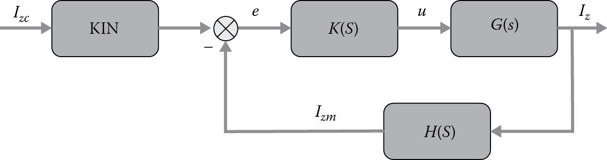
where

$G(s)=\frac{\frac{K_{act}\cdot K_1}{D\cdot kgrav}\left[-K_2\cdot s^2+1\right]}{A^{\prime }\cdot s^3+B^{\prime }\cdot s^2+C^{\prime }\cdot s+1}$ (6.23)

For the first iteration assume H(S) is unity. K(S) will be determined by the root locus method to adjust the time history properties, and KIN will be used to set the steady-state error to zero.

The root locus shown in Figure 6.34 indicates that a stable closed-loop system can be achieved when 0.01 < K < 2.7. The lower limit, K, produces a sluggish design, while the upper limit is too oscillatory with long settling times and large overshoot.

The first iteration attitude requirement set is selected to achieve a desired zero steady-state error with a time constant τ < 0.1 seconds, overshoot of <2%, and a settling time <0.2 seconds. A gain margin 5 < GM < 10 and a phase margin PM > 30° are desirable. Figure 6.35 overlays the step response time histories for 0.2 < K < 1.0.

Selecting K = 0.4 satisfies all of the first iteration preliminary design required performance parameters as shown in the associated Bode plot and step response time history in Figure 6.36 and Figure 6.37, respectively.

The next step in this design is to combine the FCS preliminary design with the guidance law(s) of choice in a nonlinear simulation and establish whether these requirements will allow the other performance requirements to be satisfied.

6.5.9.4 Guidance Law Design

The missile guidance law preliminary design and performance evaluation begins with a flow-down of kill criteria requirements and results from the preliminary seeker design and performance. Once these requirements and inputs are established, combined linear and nonlinear techniques and Monte Carlo modeling and simulation are employed. Adjoint analysis approaches [58] have historically played a significant role in this phase of design since the 1950s, but modern computational capability has enabled a more accurate Monte Carlo modeling and simulation on inexpensive desktop and laptop computers and is most recommended. In the Monte Carlo approach, guidance loop elements are often represented with transfer functions and simplified mathematical expressions. Figure 6.38 is a nonlinear guidance loop simulation block diagram with both linear and nonlinear representations of various functional components used for design and trade-off studies necessary to meet the principal objective of hitting and/or destroying the required target sets.

The missile guidance preliminary design problem, shown in yellow, is to develop a guidance law or a set of guidance laws and filtering approaches that successfully complete the terminal homing engagement. From a requirements standpoint, this means satisfying the miss distance (or hit-to-kill) requirement that flows down from the single-shot probability-of-kill, Pssk, top-level requirement with the imposed constraint of kill strategy and seeker preliminary design performance against a specific target set or sets. In following iterations, these constraints may need to be relaxed, modified, or changed after the first, and possibly subsequent, terminal homing guidance preliminary design phase(s) is completed.

There are four primary guidance law preliminary design constraints, shown in blue, to consider while addressing the primary, miss distance, design driver requirements. Specifically, guidance law design is achieved through properly characterizing, modeling, and simulating the function and performance of the guidance integrated target (GIT) factors, guidance integrated noise (GIN) factors, guidance integrated control (GIC) factors, and guidance integrated airframe (GIA) factors.

Modern guidance design is primarily based on modern estimation and control theory explicitly dealing with time-varying systems and nonstationary noise processes. The literature is exhaustive providing various modern guidance law design approaches and law performance analysis approaches (e.g., Stewart and Smith [58], Stallard [59], Yanushevsky [63], Crassidis and Junkins [64], Gurfil et al. [65], Guelman [66,67], Adler [68], Cochran et al. [69], Song [70], Yang and Yang [71], Yuan and Chern [72], Yueh [73], and Biggers [74]), and they are not repeated here. Most modern guidance design and analysis approaches employ the separation theorem (e.g., Stallard [59]) optimizing a linear guidance system quadratic performance index (e.g., mean-square miss distance) with a constraint equation where an integral-square interceptor lateral acceleration is specified. Employing the separation theorem permits the G&C problem to be divided into two subordinate problems of optimal estimation and optimal control.

Optimal estimation here is synonymous with Kalman (Kalman–Bucy) filtering [59] and is employed to produce measured state estimates of the target signal in the presence of noise, which are then acted upon by the guidance law to produce acceleration commands. Specifically, optimal estimation applies Kalman filtering to corrupted LOS, range, and their rate measurements. The GIN is assumed white, and the filtering solution is obtained from calculating the ensemble minimum mean square error of noise plus signal.

Optimal control is employed to minimize a performance index (e.g., mean-square miss distance) to produce time-dependent guidance law gains used to compute terminal homing commands necessary to close an angle and range on a dynamic target. A classical guidance law design produces fixed gains. Specifically, optimal control addresses the GIT, GIC, and GIA constraints including maintaining stability and minimizing system saturation where angular rate, position, or force limits are reached before achieving the desired guidance commands. As the time to go decreases, control saturation design issues become hard to solve and are best handled with time-varying gains. The GIA constraint, airframe time constant, is a primary design trade that will be in the trade space. The airframe time constant trade may have to be satisfied by adjustments to configuration, mass and inertia properties, and control effectiveness.

The next section covers detailed GIN sources, which are necessary to characterize, model, and simulate a complete guidance law preliminary design.

6.5.9.4.1 Guidance Integrated Noise

The guidance integrated noise (GIN) blocks shown in Figure 6.38 represent important design and performance constraints that corrupt the interceptor-to-target line-of-sight (LOS, λ) measurements. The LOS rate measurement, typically measured within seeker tracking, is accomplished in two perpendicular axes and relative to the interceptor antenna (Ax) or optics that tracks the target motion. The LOS measurement is corrupted by a variety of noise sources including glint, receiver (RCVR), and clutter (CLTR) noises that are characterized by their power spectral densities (PSD, Φ), standard deviation (STD, σ), and their correlation time constants (TN). In general, these noise sources are categorized as range dependent or independent and can be represented as shown in Figure 6.39. Fading noise is range independent and is usually easiest to filter and is not shown in Figure 6.38.

Other sources of GIN not shown are multipath error, radome boresight error (RBE), and handover error. An attempt should be made to add these error sources into the guidance law design process individually and in combination.

Multipath presents angular error due to signal reflections from surfaces being mistaken for the valid target signal. Multipath is therefore most important for look-down engagements described in the literature [60–62] and can be difficult to compensate or filter.

Radome boresight error (RBE, “R”) is defined as the rate of change of the refraction angle of the target signal with a change in the gimbal angle and is a function of radome characteristics including material type, physical dimensions, and material signal bandwidth. RBE acts to destabilize the airframe that adversely affects the missile aerodynamic design including wing size and body characteristics. Representative RBE may vary between 0.01 and 0.025 deg/deg.

Handover error comprises the heading error (HE) and time-to-go estimation error. Handover error is another source of GIN that is not shown explicitly in Figure 6.38 as it is typically accounted for in midcourse guidance; however, it could just as well be another added noise component to the LOS error. HE is the angular error measurement between the solution to the target-to-missile collision triangle and the missile velocity vector direction when terminal homing begins. Time-to-go estimation errors are the result of error on the range-to-go estimate and a combination of target and own missile velocity estimation errors. The mathematics associated with handover error was given in Chapter 5.

The Sampler, Ts block in Figure 6.38 is used to account for the receiver data collection and processing time and is a combination of a sample hold and processing delay. These values may vary between 10 and 50 ms for the sample hold and an additional 10–25 ms for a processing delay. Significant and comprehensive detail can be found on all of the GIN sources and how they are represented in modeling and simulation in the referenced literature.

6.5.9.4.1.1 Guidance Integrated Target

GIT refers primarily to the attacking target dynamics and is the primary miss distance driver of the engaging interceptor. Evasive maneuvers are one, if not the most, effective defense penetration feature (DPF) used on offensive missiles [59,61,63,72–74]. The evasive maneuver exploits the terminal homing portion of the interceptor and is typically the weakest link of the defense system attacking the engagement weapon aerodynamic time constant, potentially causing intolerable miss distances for hit-to-kill missiles/guns or causing increased miss distances that are unacceptable for warhead kill missiles. Therefore, it is of primary importance to properly characterize, model, and simulate the GIT for a guidance law preliminary design.

Target maneuver constitutes any kinematics and/or dynamics state changes in magnitude and/or direction. Regardless of the motivation of the maneuver, from a design standpoint, the target maneuver acts to evade an intercepting missile by inducing miss distance. If designed properly, an evasive maneuver can render the entire defense system ineffective despite whether or not all of the other defense system elements are doing their job. A properly designed evasive defense penetration maneuver is the maneuver that causes the defensive weapon to miss with sufficient distance that no damage is caused to the evading target while yet not prohibiting target from accomplishing its mission.

Evasive maneuver design parameters include weave magnitude, weave period (for a weaving evasion) initiation time, and duration. The preliminary flow-down design requirement is to minimize the effect of practical evasive maneuvers, and therefore, the bandwidths of potential evasive maneuver design parameters are important inputs to the guidance and control preliminary design.

Unfortunately, it is difficult to build a general analytical model which is well matched to reality and that can be utilized during design. Statistical models are most readily used [58,59,63,64,72,74] and have their place in the design process but in general lack the dynamic or physics-based limitations imposed on the evading missile that are typically imposed on the intercepting missile in the form of time constants. The design results are then pessimistic from the weapon designer’s perspective leading to potentially unnecessary trades and compromises. To design the estimator, the target is modeled using a statistical process approach, but when implemented within the homing model, the target will need to be a more accurate representation.

A more appropriate preliminary design approach concerning target evasive maneuver is to characterize the requirements using a two-part process. The first part is to establish the maneuver design permissive bounds (MDPBs) of potential offensive target designs or the maneuver magnitude limit requirement in a capability-based acquisition. The second part is an optimization problem. Formally, it should first be determined what target magnitude capability should the defensive system be capable of successfully engaging and then what would be the optimal maneuver characteristics given a target class.

The MDPB objective is to bound the maximum achievable, range-sensitive maneuver magnitude–period combinations. These combinations are a function of initiation and duration times and are variable with dynamic pressure. Next, interceptor miss distance is significantly influenced by evasive maneuver weave frequency, and it can be shown that there exists a frequency for which the amplitude of the miss is a maximum [63].

The preliminary guidance law design and performance analysis should proceed using identically commensurate dynamics for both the evader and pursuer. A reasonable first approach is to employ a low-order equivalent model (LOEM) in the homing loop model characterized in second order by the airframe natural frequency and damping and a first-order flight control system time constant. Tail-controlled missiles should include the right-half plane zero (nonminimum phase systems). An example LOEM is given in the following equation:

$W(s)=\frac{1-\frac{s^2}{{\omega }_z^2}}{(1+\tau s)\left(1+\frac{2\zeta }{{\omega }_{af}}s+\frac{s^2}{{\omega }_{{}_{af}}^2}\right)}$ (6.24)

Accordingly, a closed-form solution for miss distance can be obtained by Yanushevsky [63] as a function of the guidance law under study and the effective navigation parameters, guidance system time constant, natural frequency, and damping ratio to determine the optimal weave frequency for which the amplitude of the miss distance has a maximum. The established existence and the procedure of determining the miss distance maximizing weaving frequency offer the optimization approach to the design of the worst-case scenario when developing defensive missiles to defeat maneuvering targets. Figure 6.40 shows an example of the results for determining the optimal evasive maneuver weave frequency for an interceptor modeled with the given parameters [63].

The results from this phase are inputs for preliminary design utilizing a planar 2D Monte Carlo model. The results from the planar model and simulation once an apparent acceptable preliminary design is achieved will be made more precise by utilizing detailed nonlinear six-degree-of-freedom engagement models.

6.5.9.4.1.2 Guidance Integrated Control

The GIC module receives the guidance law acceleration command and represents the flight control system (FCS) response. It is important to represent the FCS time delay and time-dependent response magnitude accurately. This is best accomplished using transfer functions. The nonlinear limiting of the command and response must also be included in this modeling to pick up saturation levels and realistic airframe limits.

6.5.9.4.1.3 Guidance Integrated Airframe

The GIA is represented by a pair of transfer functions for the missile body angular rate response and the missile c.g. acceleration response to control deflections. It is in the second-order airframe dynamics transfer function that an accurate representation of airframe time constant is required. The second-order airframe kinematics block must represent both the normal/lateral interceptor c.g. acceleration and its axial acceleration or slow-down effects. Oftentimes, airframe slow-down is neglected in guidance law design and analysis, which is a mistake. Slow-down is a major contributor to miss distance and is therefore an important parameter in designing the guidance law and its implementation. Airframe slow-down within the pitch plane can be represented in a simplified fashion as shown in the following equations:

${\dot{V}}_M=\left[\frac{Thrust-D_{ZL}}{W}\cos \alpha -{\eta }_M\sin \alpha \right]$ (6.25)

$\dot{\gamma }=\frac{9.81}{V_M}\left[\frac{Thrust-D_{ZL}}{W}\sin \alpha +{\eta }_M\cos \alpha \right]$ (6.26)

The term DZL represents the zero-lift drag and not axial force and ηM represents normal (or lateral when using β) acceleration in g’s. The angle of attack, α, can be represented as

$\alpha ={\tau }_{\alpha }\cdot \dot{\gamma }$ (6.27)

The airframe time constant (τα) equation was given in Table 6.2.

Homing analysis when high-frequency guidance signals are expected requires a model of the interceptor body-bending modes. Hemsch and Nielsen [15] provides a detailed treatment of how to handle missile body-bending modes in flight control system analysis and could apply for preliminary design. Guidance law preliminary design does not necessarily require this analysis unless during a particular design trial it is discovered that high-frequency commands are necessary. If this is the case, see Hemsch and Nielsen [15].

6.5.7.9.1.4 Estimation

As discussed in the preceding sections, the noise sources, disturbances, and modeling inaccuracies corrupt the measurements that are intended for use in the guidance law design and performance analysis. To prepare the preliminary design problem of Figure 6.38, an estimator needs to be designed. This estimator will no doubt be iteratively changed in the preliminary design process. The Kalman–Bucy filtering (KBF) approach is a commonly used filter and will be implemented here. KBF is based on a probabilistic treatment of process and measurement noise sources, and therefore, the probability theory is used to model the corruption and uncertainty sources in a Monte Carlo sense described earlier. Essentially, the KBF is used to reconstruct the measured states from the noisy measurements. The KBF is usually a good choice for guidance applications because it is fundamentally a low-pass filter where legitimate guidance measurements will have a relatively low frequency while unwanted disturbances and noise typically have a high frequency. The literature on this subject is exhaustive and should be consulted for implementation.

6.5.9.4.1.5 Mathematical Guidance Law Design

The context of this discussion on missile guidance law design is within the terminal homing portion of the engagement. It is assumed that a midcourse guidance law was implemented and handover errors exist during the transition from midcourse to terminal homing and that some relatively short terminal homing time period remains to zero-out miss distance. Based on terminal engagement encounter conditions (requirements) and the flow-down of requirements, a mathematical guidance law will have to be selected to satisfy the kill criteria. The guidance law is selected based on a series of trade-offs between AMD system engagement envelope and Pssk performance requirements and the cost and complexity of implementation. The objective of the guidance law is to mathematically produce commands from relative target-to-interceptor state measurements that are translated into actuator control signals that steer the interceptor into a collision course with the target while minimizing the amount of energy expended. It is likely that more than one guidance law algorithm will be required to fulfill the interceptor engagement encounter envelope requirements.

The most widely used terminal guidance law is proportional navigation (PN). PN is the optimal intercept solution minimizing the minimum mean-square miss distance plus the weighted integral square interceptor acceleration perpendicular to the LOS vector for a constant closing velocity, nonmaneuvering target. PN was established as a guidance law in the 1940s and received the focus of attention when intercept missiles became prevalent in the 1950s, and since this time, there has been no other single guidance law that is the center of continued practical research and development. Today, PN is the established guidance law benchmark for both nonmaneuvering and maneuvering target engagements.

The applied principle of PN is that a mathematically generated acceleration command steers the interceptor velocity vector to nullify the interceptor-to-target LOS rate. PN performance varies with choices of design parameters including steering gain, navigation gain, and additive terms, all of which may or may not change with time to go. Moreover, either linear or nonlinear implementations of PN may be used singularly or in combination. When PN is solely dependent on relative angle rate information, it is easy to mechanize but is directly tied to the seeker angle tracking mechanization and the associated tracking errors. As such, the PN algorithm design will be closely tied to the angle tracking error and error mitigation design approaches. The selection of these design parameters will be discussed in the remainder of this section.

Much of the PN design work in the last 40 years has been to improve performance against maneuvering targets and in variable closing velocity engagements. PN implementations fall in one of two classes [65–67], either the true proportional navigation (TPN) or the pure proportional navigation (PPN) law class. TPN generates a maneuver acceleration command perpendicular to the instantaneous LOS. PPN generates a maneuver acceleration perpendicular to the instantaneous velocity vector. The difference between TPN and PPN is in the calculation of the effective navigation constant N’ in the following equation’s PN command representation:

${\eta }_c=N^{\prime }\cdot V_c\cdot \dot{\lambda }$ (6.28)

where

$N^{\prime }=\{\begin{array}{c}N\cdot V_M\cdot \cos ({\gamma }_M-\lambda )/V_C\Rightarrow PPN\\ N\cdot V_M/V_C\Rightarrow TPN\end{array}$ (6.29)

The effective navigation constant can take on values 2 ≤ N′ < 5 to generate a collision course typically without violating stability requirements.

As part of the preliminary design process, maintaining stability throughout the engagement is an added criterion. As the range to go decreases, the problem of maintaining guidance law stability severely increases and will adversely affect miss distance and therefore is a primary design driver. Within the context of preliminary design when dealing with a roll attitude–stabilized missile, it is reasonable to assume that the directional planes are decoupled and can be modeled independently to accomplish the objectives, and typically, this design work is accomplished in decoupled planes. Therefore, due to its simplicity, much of the work on PN has been accomplished in single plane analysis. Arguably, using a 3D PN preliminary design approach will produce different and more accurate results and may be appropriate for the later stages of preliminary design. The mathematical model for the 3D engagement with PN is cumbersome but can be found in the literature (see, e.g., Adler [68], Cochran et al. [69], Song [70], and Yang and Yang [71]).

Other linear and nonlinear forms of PN have been produced in the literature to address some of the inherent vulnerabilities in the PN guidance law assumptions to include constant closing velocities, nonmaneuvering targets, and short-range instability. These vulnerabilities in the law have been the focus of much research and have produced improvements to the original classical PN law. For example, an additional PN approach, realistic true proportional navigation (R-TPN), has been proposed in the literature [72]. R-TPN requires the use of active radar Doppler processing to measure the effects due to nonconstant closing velocities. These closing velocity measurements are incorporated into the law through time-varying gain adjustments.

When considering improvements regarding maneuvering targets, there have been many new PN formulations. One of the linear forms of PN developed to address the maneuvering target is augmented proportional navigation (APN). APN is the optimal control law, where the miss distance criteria go to zero having a minimum integral-squared interceptor acceleration constraint, for a noise-free, zero-lag guidance system against a target executing an instantaneous step maneuver perpendicular to the interceptor-to-target LOS. The APN is written in Equation 6.21:

${\eta }_c=N^{\prime }\cdot V_c\cdot \dot{\lambda }+\frac{N^{\prime }{\eta }_T}{2}$ (6.30)

The step target maneuver in the previous equation is represented by ηT.

The APN has shown promise to improve homing performance in some limited cases against maneuvering targets as would the theoretical development of the law suggest. APN homing performance improvement over PN is tightly tied to target maneuver estimation performance and the minimization of guidance lags. One such APN practical implementation is presented by Yueh [73].

The most practical and useful way to address maneuvering targets and to account for guidance system lags is to modify the PN guidance law by adding lead and nonlinear PN terms. The lead term in the modified law will inherently reduce the effects of the dominant guidance system lag terms, while the nonlinear term(s) if selected properly can be used to weigh the error signal, most notably LOS rate in PN, to reduce the effects of highly evasive target maneuvers that are typically oscillatory in nature. Neither guidance system lags nor oscillatory maneuvers are assumed in the APN law derivation.

The LOS rate measurement from the angle track loop can be modified with a lead term filter as shown in Figure 6.41.

The resulting transfer function is provided in Equation 6.31, where τA (τA = 1/K1) is the angle track loop time constant:

$\frac{{\upsilon }_s}{\dot{\lambda }}=\frac{{\tau }_{2}s+1}{{\tau }_A\cdot {\tau }_1\cdot {\tau }_2{s}^3+{\tau }_A\cdot \left({\tau }_1+{\tau }_2\right)s^2+{\tau }_A\cdot s+1}$ (6.31)

The trade space with this filter has higher sensitivity to radome boresight error and premature loss of stability and is more sensitive to glint or scintillation, increasing miss distance due to these sources. The parameters τ1 and τA are chosen based on S:N and τ2 will be small so as to improve damping due to noise. K2 is 1 or greater. The value υ is used as the noisy LOS rate and passed to the Kalman filter for estimation.

Nonlinear PN was investigated by Biggers [74] as early as 1969, to improve the capabilities of PN to countertarget evasive oscillatory maneuvers. Biggers offered the following equation as PN with a nonlinear modification term without any mathematical derivation:

$\dot{\gamma }={N^{\prime }}_1\dot{\lambda }+{N^{\prime }}_n{\dot{\lambda }}^n$ (6.32)

When the previous equation is multiplied by VC, it returns the usual acceleration command of pure or true PN. The new guidance law proposed that “n” be an odd integer. By inspection when the LOS rate is large, it is weighted more heavily, and as it approached zero, the desired condition, it nearly disappears and defaults to the traditional PN. The nonlinear term causes large LOS rates to be corrected rapidly. Preliminary results obtained by Biggers show marked miss distance improvement against sinusoidal maneuvering targets employing Equation 6.32 when n = 3 over traditional PN.

A rigorous derivation and new nonlinear guidance (NLG) law design approach was offered by Yanushevsky and Boord [75] where the optimality of the cubic LOS rate term was proven using Lyapunov control techniques and additionally proves the optimality of the well-known PN guidance law against nonmaneuvering targets. The new NLG laws developed by Yanushevsky and Boord [75] improve interceptor homing performance against maneuvering targets when compared to PN and APN guidance laws without requiring any additional information from the sensor. The nonlinear guidance laws take the form shown in Equation 6.33. The first term is the classic PN term, the second term (third solution) is nonlinear, and so on:

$\begin{array}{l}{\eta }_c=N\cdot v_c\cdot \dot{\lambda }+{\displaystyle \sum _{k=1}^3{u}_k}\Rightarrow k=1,3,5,7,\dots \\ u_1=N_1\cdot {\dot{\lambda }}^3\left(t\right)\\ u_3=N_3\cdot a_T\left(t\right)\end{array}$ (6.33)

A 3D derivation of this NLG law is provided by Yanushevsky [76].

References

1. Warren, R.S., Price, C.F., Gelb, A., and Vander Velde, W.E., Direct statistical evaluation of nonlinear guidance systems, in AIAA Guidance and Control Conference, Paper No. 73-836, Seattle, WA, August 20–22, 1973.

2. Calamia, M., Jiberio, R., Franleschetti, G., and Givli, D., Radar tracking of low altitude targets, IEEE Transactions on Aerospace and Electronic Systems, AES-10, 539–544, 1974.

3. Nesline, W.F., Missile guidance for low altitude air defense, AIAA Journal Guidance, Control, and Dynamics, 2(4), 283–289, July–August 1979.

4. Tsuchiya, T. and Takashige, M., Optimal conceptual design of two-stage reusable rocket vehicles including trajectory optimization, Journal of Spacecraft and Rockets, 41(5), 770–7789, September–October 2004.

5. Fleeman, E.L., Tactical Missile Design, AIAA Education Series, 2nd edn., AIAA, Reston, VA, July 2002.

6. Fleeman, E.L. and Donatelli, G.A., Conceptual Design Procedure Applied to a Typical Air Launched Missile, AIAA-81-1688, Dayton, OH, August 11–13, 1981.

7. Chin, S.S., Missile Configuration Design, McGraw-Hill, New York, 1961.

8. Blake, W.B., Missile DATCOM, AFRL-VA-WP-TR-1998-3009, February 1998.

9. Moore, F.G. and Moore, L.Y., The AP09, Report Number A365574, January 2008.

10. Nesline Jr., W.F. and Nesline, M.L., Wing size versus radome compensation in aerodynamically controlled radar homing missiles, AIAA Paper 85-1869, Reston, VA, 1985.

11. Moore, F.G., Approximate Methods for Weapon Aerodynamics, Progress in Astronautics and Aeronautics Series, V-186, AIAA, Reston, VA, 2000.

12. Slack, A.J., Unpublished work and presentation, Battlespace engineering assessment tool, Technology Service Corporation, Silver Spring, MD, 2002.

13. Krieger, R.J. and Williams, J.E., High performance missiles of the future, McDonnell Douglas Astronautics Company, Neilson Engineering Research, St, Santa Clara, CA, 1988.

14. Nielsen, J.N., The Present Status and the Future of Missile Aerodynamics, NASA Technical Memorandum, Moffett Field, CA, January 1988.

15. Hemsch, M.J. and Nielsen, J.N., Aerodynamic Considerations for Autopilot Design, Tactical Missile Aerodynamics, Vol. 104, Progress in Astronautics and Aeronautics, AIAA, New York, 1986 (Chapter 1, Cronvich, L.L.).

16. Wise, K.A. and Broy, D.J., Agile missile dynamics and control, AIAA Journal of Guidance, Control and Dynamics, 21(3), 441–449, May–June 1998.

17. Sutton, G.P. and Biblarz, O., Rocket Propulsion Elements, 7th edn., John Wiley & Sons, New York, 2001.

18. Briggs, M.M. and Tahk, M.-J., Appropriate aeroprediction accuracy in defining missile systems for aerodynamic flight, in NEAR Conference on Aerodynamics, Paper No. 4, Neilsen Engineering and Research, Monterey, CA, 1988.

19. Fleeman, E.L., Technologies for future precision strike missile systems-missile aeromechanics technology, in presented at the RTO SCI Lecture Series on Technologies for Future Precision Strike Missile Systems, RTO-EN-018, Paris, France, June 18–19, 2001.

20. James, D.A., Radar Homing Guidance for Tactical Missiles, Macmillan Education, Basingstoke, UK, 1986.

21. Maksimov, M.V. and Gorgonov, G.I., Electronic Homing Systems, Artech House, Norwood, MA, 1988.

22. Edde, B., RADAR Principles, Technology and Applications, Prentice Hall, Englewood Cliffs, NJ, 1993.

23. Barton, D.K., Radar System Analysis, Prentice Hall, Englewood Cliffs, NJ, 1964.

24. Weidler, R.D., Target LOS and seeker head equations for an AAM simulation, Flight Dynamics Group, Stability and Flight Control Section, FZE-977, November 19, 1969.

25. Hendeby, G., Development and evaluation of an active radio frequency seeker model for missile with data-link capability, LiTH-ISY-EX-3309-2002, December 11, 2002.

26. The George Washington University, School of Engineering, Modern air-to-air radar systems, A short course, Washington, DC, April 26–29, 1983.

27. Nathanson, F.E. and Jones, W., Airborne radar, an intensive short course, Technology Service Corporation, Silver Spring, MD, Circa 1980.

28. Schleher, D.C., Introduction to Electronic Warfare, Artech House, Dedham, MA, 1986.

29. Miwa, S., Imado, F., and Kuroda, T., Clutter effect on the miss distance of a radar homing missile, AIAA Journal of Guidance, Control and Dynamics, 11(4), 336–342, July–August 1988.

30. Mitchell, R.L. and Walker, J.F., Recursive methods for computing detection probabilities, IEEE Transactions on Aerospace and Electronic Systems, AES-7(4), 671–676, July 1971.

31. Shnidman, D.A., Radar detection probabilities and their calculation, IEEE Transactions on Aerospace and Electronic Systems, AES-31(3), 928–950, July 1995.

32. Sandhu, G.S., A real time statistical radar target model, IEEE Transactions on Aerospace and Electronic Systems, AES-21(4), 490–507, July 1985.

33. Huynen, J.R., McNolty, F., and Hansen, E., Component distributions for fluctuating targets, IEEE Transactions on Aerospace and Electronic Systems, AES-11(6), 1316–1331, November 1975.

34. Nesline, W. and Zarchan, P., Radome induced miss distance in aerodynamically controlled homing missiles, in AIAA Guidance Navigation and Control Conference Proceedings, Paper No. 84-1845, Seattle, WA, 1984, pp. 99–115.

35. Borden, B., What Is the Radar Tracking “Glint” Problem and Can It Be Solved, Naval Air Warfare Center Weapons Division, China Lake, CA, NAWCWPNS TP 8125, May 1993.

36. Gordon, N. and Whitby, A., Bayesian approach to guidance in the presence of glint, AIAA Journal of Guidance, Control and Dynamics, 22(3), 478–485, May–June 1999.

37. Nesline, F.W. and Zarchan, P., Miss distance dynamics in homing missiles, AIAA Guidance and Control Conference Proceedings, Paper No. 84-1844, Snowmass, CO, pp. 84–98, 1984.

38. Garnell, P. and East, D.J., Guided Weapon Control Systems, Pergamon Press, Oxford, UK, 1977.

39. Trapp, R.L., Pulse Doppler radar characteristics, limitations and trends, The JHU/APL, Howard County, MD, FS-84-167, October 1984.

40. Farrell, J.L. and Taylor, R.L., Doppler radar clutter, IEEE Transactions on Aerospace and navigational Electronics, ANE-11(3), 162–172, September 1964.

41. Skolnik, M.I., Radar Handbook, McGraw-Hill, New York, 1970.

42. Marcum, J.I. and Swerling, P., Studies of target detection by pulsed radars, IRE Transactions on Information Theory, IT-6(2), 59–308, April 1960.

43. Swerling, P., Recent developments in target models for radar detection analysis, in presented at the AGARD Avionics Technical Symposium on Advanced Radar Systems, Istanbul, Turkey, May 25–29, 1970.

44. Xin, M. et al., Nonlinear bank-to-turn/skid-to-turn missile outer-loop/inner-loop autopilot design with θ-D techniques, in AIAA Guidance Navigation and Control Conference Proceedings, Austin TX, August 11–13, 2003.

45. Wassom, S.R. and Faupell, L.C., Integrated aerofin/thrust vector control for tactical missiles, AIAA Journal of Propulsion, 7(3), 374–381, May–June 1991.

46. Roskam, J., Airplane Flight Dynamics and Automatic Flight Controls, Part II, Roskam Aviation and Engineering Corporation, Ottawa, KS, 1979.

47. Nachtigal, C.L., Instrumentation and Control, Fundamentals and Applications, Wiley Series in Engineering Practice, John Wiley & Sons, New York, 1990.

48. Goldshine, G.D. and Lacy, G.T., High-response electromechanical control actuator, in JPL Proceedings of the Third Aerospace Mechanisms Symposium, Pasadena, CA, October 1, 1968, pp. 19–26.

49. Wingett, P.T. et al., Flight control actuation system, U.S. Patent 6,827,311 B2, December 7, 2004.

50. Denel Sales Brochure, Servo actuators, Broc0253.CDR, October 2007.

51. Knauber, R.N., Computer program for post-flight evaluation of the control surface response for an attitude controlled missile, NASA Contractor Report 166032, Hampton, VA, November 1982.

52. Abzug, M.L., Computational Flight Dynamics, AIAA Education Series, American Institute of Aeronautics and Astronautics, Reston, VA, 1998.

53. Blakelock, J.H., Automatic Control of Aircraft and Missiles, 2nd edn., John Wiley & Sons, New York, 1991.

54. Wise, K.A. and Broy, D.J., Agile missile dynamics and control, AIAA Journal of Guidance, Control and Dynamics, 21(3), 441–449, May–June 1998.

55. Wise, K.A., Comparison of six robustness tests evaluating missile autopilot robustness to uncertain aerodynamics, AIAA Journal of Guidance, Control and Dynamics, 15(4), 861–870, July–August 1992.

56. Wise, K.A., Missile autopilot robustness using the real multiloop stability margin, AIAA Journal of Guidance, Control and Dynamics, 16(2), 354–362, March–April 1993.

57. Bar-On, J.R. and Adams, R.J., Linearization of a six degree[s]-of freedom missile for autopilot analysis, AIAA Journal of Guidance, Control and Dynamics, 21(1), 184–187, 1998.

58. Stewart, E.C. and Smith, G.L., The Synthesis of Optimum Homing Missile Guidance Systems with Statistical Inputs, NASA Memo 2-13-59A, Ames Research Center, Moffett Field, CA, April 1959.

59. Stallard, D.V., Classical and Modern Guidance of Homing Interceptor Missiles, Raytheon Company-Seminar of Department of Aeronautics and Astronautics, Massachusetts Institute of Technology, Cambridge, MA, April 1968.

60. Calamia, R.J., Franleschetti, G., and Givli, D., Radar tracking of low altitude targets, IEEE, Transactions Aerospace and Electronic Systems, AES-10(4), 543–549, 1974.

61. Nesline, F.W., Missile guidance for low-altitude air defense, AIAA Journal of Guidance, Control, and Dynamics, 2(4), 283–289, July–August 1979.

62. Bucco, D. and Hu, Y., A comparative assessment of various multipath models for use in missile simulation studies, in AIAA Modeling and Simulation Technologies Conference and Exhibition, AIAA-2000-4286, Denver, CO, August 14–17, 2000.

63. Yanushevsky, R., Modern Missile Guidance, CRC Press, Taylor & Francis Group, Boca Raton, FL, 2008.

64. Crassidis, J.L. and Junkins, J.L., Optimal Estimation of Dynamic Systems, Applied Mathematics and Nonlinear Science Series, Chapman & Hall/CRC Press, Boca Raton, FL, 2004.

65. Gurfil, P., Jodorkosky, M., and Guelman, M., Finite time stability approach to proportional navigation systems analysis, AIAA Journal of Guidance, Control and Dynamics, 21(6), 853–861, November–December 1998.

66. Guelman, M., A qualitative study of proportional navigation, IEEE Transactions on Aerospace and Electronic Systems, AES-7(4), 637–643, July 1971.

67. Guelman, M., The closed form solution of true proportional navigation, IEEE Transactions on Aerospace and Electronic Systems, AES-12(4), 472–482, July 1976.

68. Adler, F.P., Missile guidance by three dimensional proportional navigation, Journal of Applied Physics, 27(5), 500–507, May 1956.

69. Cochran, J.E., No, T.S., and Thaxton, D.G., Analytical solutions to a guidance problem, AIAA Journal of Guidance, Control and Dynamics, 14(1), 117–122, January–February 1991.

70. Song, S., A Lyapunov-like approach to performance analysis of 3-dimensional pure PNG laws, IEEE Transactions on Aerospace and Electronic Systems, 30(1), 238–247, January 1994.

71. Yang, C.D. and Yang, C.C., Analytical solution of generalized three-dimensional proportional navigation, AIAA Journal of Guidance, Control and Dynamics, 19(3), 569–577, May–June 1996.

72. Yuan, P.J. and Chern, J.S., Solutions of true proportional navigation for maneuvering and non-maneuvering targets, AIAA Journal of Guidance, Control and Dynamics, 15(1), 268–271, January–February 1992.

73. Yueh, W.R., Augmented proportional navigation in third-order predictive scheme, U.S. Patent 4,502,650, March 5, 1985.

74. Biggers, E.L., Air-to-air missile guidance and control, Unpublished Technical Memorandum, July 10, 1969.

75. Yanushevsky, R.T. and Boord, W.J., New approach to guidance law design, AIAA Journal of Guidance, Control and Dynamics, 28(1), 162–166, January–February 2005.

76. Yanushevsky, R.T., Concerning Lyapunov-based guidance, AIAA Journal of Guidance, Control and Dynamics, 29(2), 509–511, March–April 2006.

77. Blake, L., Radar Range-Performance Analysis, Munro Publishing Company, Silver Spring, MD, p.39, 1991.