3 Approximate membership: Bloom and quotient filters

This chapter covers

• Learning what Bloom filters are and why and when they are useful
• Configuring a Bloom filter in a practical setting
• Exploring the interplay in Bloom filter parameters
• Learning about quotient filters as Bloom filter replacements
• Comparing the performance of a Bloom filter and a quotient filter

Bloom filters have become a standard in systems that process large datasets. Their widespread use, especially in networks and distributed databases, comes from the effectiveness they exhibit in situations where we need a hash table functionality but do not have the luxury of space. They were invented in the 1970s by Burton Bloom [1], but they only really “bloomed” in the last few decades due to an increasing need to tame and compress big datasets. Bloom filters have also piqued the interest of the computer science research community, which developed many variants on top of the basic data structure in order to address some of the filters’ shortcomings and adapt them to different contexts.

One simple way to think about Bloom filters is that they support insert and lookup in the same way that hash tables do, but using very little space (i.e., 1 byte per item or less). This is a significant savings when keys take up 4-8 bytes. Bloom filters do not store the items themselves, and they use less space than the lower theoretical limit required to store the data correctly; therefore, they exhibit an error rate. They have false positives, but they do not have false negatives, and the one-sidedness of the error can be used to our benefit. When the Bloom filter reports the item as Found/Present, there is a small chance it is not telling the truth, but when it reports the item as Not Found/Not Present, we know it’s telling the truth. In situations where the query answer is expected to be Not Present most of the time, Bloom filters offer great accuracy plus space-saving benefits.

For instance, Bloom filters are used in Google’s WebTable [2] and Apache Cassandra [3], which are among the most widely used distributed storage systems for handling massive data. Namely, these systems organize their data into a number of tables called sorted string tables (SSTs) that reside on disk and are structured as key-value maps (e.g., a key might be a URL, and a value might be website attributes or contents). WebTable and Cassandra simultaneously handle adding new content into tables and answering queries, and when a query arrives, it is important to locate the SST containing the queried content without explicitly querying each table. To that end, dedicated Bloom filters in RAM are maintained, one per SST, to route the query to the correct table.

In the example shown in figure 3.1, we are given 50 SSTs on disk and 50 associated Bloom filters in RAM. As soon as the Bloom filter reports Not Present on a lookup, the query is routed to the next Bloom filter. The first time a Bloom filter reports the item as Present (in this example, SST3’s Bloom filter), we go to disk to check if the item is present in the table. In the case of a false alarm, we continue routing the query until a Bloom filter reports Present and the data is also found on disk and returned to the user, as with SST50.

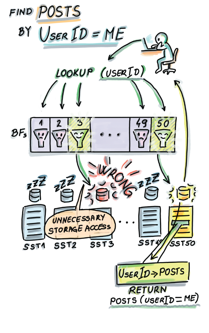
Figure 3.1 Bloom filters in distributed storage systems. In this example, we have 50 SSTs on disk, and each table has a dedicated Bloom filter that can fit into RAM due to its much smaller size. When a user does a lookup, the lookup first checks the Bloom filters, thus avoiding expensive disk seeks.

Bloom filters are most useful when placed strategically in high-ingestion systems. For example, having an application perform an SSD/disk read/write can easily bring down the throughput of an application from hundreds of thousands of ops per second to only a couple of thousand or even a couple of hundred ops/sec. If we place a Bloom filter in RAM to serve the lookups instead, we can avoid this performance slump and maintain consistently high throughput across different components of an application. More details on how Bloom filters are integrated in the bigger picture of streaming systems will be given in chapter 6.

In this chapter, you will learn how Bloom filters work and when to use them, with various practical scenarios as examples. You will also learn how to configure the parameters of the Bloom filter for your particular application. There is an interesting interplay between the space (m), number of elements (n), number of hash functions (k), and the false positive rate (f). For readers who are more mathematically inclined, we will spend some time understanding where the formulas relating important Bloom filter parameters come from and whether one can do better than the Bloom filter.

In section 3.7, we will explore a very different data structure that is functionally similar to Bloom filters. A quotient filter [4] is a compact hash table that offers space-saving benefits at the cost of false positives, but also offers other advantages. If you are confident in your knowledge of Bloom filters, skip to section 3.7.

3.1 How it works

Bloom filters have two main components:

• A bit array A[0..m-1], with all slots initially set to 0

• k independent hash functions h₁, h₂, ..., h_k, each mapping keys uniformly randomly onto a range [0, m - 1]

3.1.1 Insert

To insert an item x into the Bloom filter, we first compute the k hash functions on x, and for each resulting hash, set the corresponding slot of A to 1 (see pseudocode and figure 3.2):

Bloom_insert(x):
    for i ← 1 to k  
        A[hi(x)] ← 1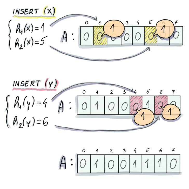

Figure 3.2 Example of an insert into a Bloom filter. In this example, an initially empty Bloom filter has m = 8 and k = 2 (two hash functions). To insert an element x, we first compute the two hashes on x, the first of which generates 1 and the second 5. We proceed to set A[1] and A[5] to 1. To insert y, we also compute the hashes and similarly set positions A[4] and A[6] to 1.

3.1.2 Lookup

Similar to insert, lookup computes k hash functions on x, and the first time one of the corresponding slots of A equals 0, the lookup reports the item as Not Present; otherwise it reports the item as Present:

Bloom_lookup(x):
    for i ← 1 to k  
        if(A[hi(x)] = 0)
            return NOT PRESENT
    return PRESENT

Figure 3.3 shows an example of a lookup on the resulting Bloom filter from figure 3.2 and how it can generate true positives (on element x that was actually inserted) and false positives (on element z that was never inserted).

Figure 3.3 Example of a lookup on a Bloom filter. To do a lookup on x, we compute the hashes (which are the same as in the case of an insert), and we return Found/Present, as both bits in corresponding locations equal 1. Then we do a lookup of an element z, which we never inserted, and its hashes are respectively 4 and 5, and bits at locations A[4] and A[5] equal 1; thus, we again return Found/Present.

As seen in figure 3.3, false positives can occur when some other elements together set the bits of some other element to 1 (in this example, two previous items, x and y, have set z’s bit locations to 1).

Asymptotically, the insert operation on the Bloom filter costs O(k). Considering that the number of hash functions rarely goes above 12, this is a constant-time operation. The lookup might also need O(k) in case the operation has to check all the bits, but most unsuccessful lookups will give up way before then; we will see that, on average, an unsuccessful lookup in a well-configured Bloom filter takes about one to two probes before giving up. This makes for an incredibly fast lookup operation.

3.2 Use cases

In the chapter introduction, we saw the application of Bloom filters to distributed storage systems. In this section, we will see more applications of Bloom filters to distributed networks: the Squid network proxy and the Bitcoin mobile app.

3.2.1 Bloom filters in networks: Squid

Squid is a web proxy cache. Web proxies use caches to reduce web traffic by maintaining a local copy of recently accessed links from which they can serve clients’ requests for webpages, files, and so on. One of the protocols [5] suggests that each proxy also keeps a summary of the neighboring proxies’ cache contents and checks the summaries before forwarding any queries to neighbor proxies. Squid implements this functionality using Bloom filters called cache digests (https://wiki.squid-cache.org/SquidFaq/AboutSquid) (see figure 3.4).

Figure 3.4 Bloom filter in Squid web proxy. A user requests a web page x, and a web proxy A cannot find it in its own cache, so it locally queries the Bloom filters of B, C, and D. The Bloom filter for D reports Present, so the request is forwarded to D. The resource is found at D and returned to the user.

Cache contents frequently go out of date, and Bloom filters are occasionally broadcasted between the neighbors. Because Bloom filters are not always up to date, false negatives can arise when a Bloom filter claims the element is present in a proxy but the proxy no longer contains the resource.

3.2.2 Bitcoin mobile app

Peer-to-peer networks use Bloom filters to communicate data, and a well-known example of this is Bitcoin. An important feature of Bitcoin is ensuring transparency between clients, which is ensured by having each node be aware of everyone’s transactions. However, for nodes that are operating from a smartphone or a similar device of limited memory and bandwidth, keeping a copy of all transactions is highly impractical, so Bitcoin offers the option of simplified payment verification (SPV), where a node can choose to be a light node by advertising a list of transactions it is interested in. This is in contrast to full nodes that contain all the data (figure 3.5).

Figure 3.5 In Bitcoin, light clients can broadcast what transactions they are interested in and thereby block the deluge of updates from the network.

Light nodes compute and transmit a Bloom filter of the list of transactions they are interested in to the full nodes. This way, before a full node sends information about a transaction to the light node, it first checks its Bloom filter to see whether a node is interested in it. If a false positive occurs, the light node can discard the information upon its arrival [6].

More recently, Bitcoin has also offered other methods of transaction filtering with improved security and privacy properties.

3.3 A simple implementation

A basic Bloom filter is fairly straightforward to implement. We show a simple implementation that uses a Python wrapper for MurmurHash, mmh3, which we discussed in chapter 2. By setting k different seeds, we are able to obtain k different hash functions. The implementation also uses bitarray, a library that allows space-efficient encoding of the filter you need to install to run the code:

import math
import mmh3
from bitarray import bitarray
 
class BloomFilter:
    def __init__(self, n, f):    ❶
        self.n = n
        self.f = f
        self.m = self.calculateM()
        self.k = self.calculateK()
 
        self.bit_array = bitarray(self.m)
        self.bit_array.setall(0)
        self.printParameters()
 
    def calculateM(self):
        return int(-math.log(self.f)*self.n/(math.log(2)**2))
 
    def calculateK(self):
        return int(self.m*math.log(2)/self.n)
 
    def printParameters(self):
        print("Init parameters:")
        print(f"n = {self.n}, f = {self.f}, m = {self.m}, k = {self.k}")
 
    def insert(self, item):
        for i in range(self.k):
            index = mmh3.hash(item, i) % self.m
            self.bit_array[index] = 1
 
    def lookup(self, item):
        for i in range(self.k):
            index = mmh3.hash(item, i) % self.m
            if self.bit_array[index] == 0:
                return False
 
        return True

❶ Provide the number of elements and the desired false positive rate.

You can try out the implementation by inserting a couple of items of type string:

    bf = BloomFilter(10, 0.01)
    bf.insert("1")
    bf.insert("2")
    bf.insert("42")
    print("1 {}".format(bf.lookup("1")))
    print("2 {}".format(bf.lookup("2")))
    print("3 {}".format(bf.lookup("3")))
    print("42 {}".format(bf.lookup("42")))
    print("43 {}".format(bf.lookup("43")))

The constructor of this sample implementation lets the user set the maximum number of elements (n) and the desired false positive rate (f), while the constructor does the job of setting two other parameters (m and k). This is a common choice, as we often know how large of a dataset we’re dealing with and how high of a false positive rate we are willing to admit. To understand how the remaining parameters are set in this implementation and how to configure a Bloom filter to get the most bang for your buck, read on.

3.4 Configuring a Bloom filter

First, we outline main formulas relating important parameters of the Bloom filter. We use the following notation for the four parameters of the Bloom filter:

• n = number of elements to insert

• f = the false positive rate

• m = number of bits in a Bloom filter

• k = number of hash functions

The formula that determines the false positive rate as a function of the other three parameters is as follows (equation 3.1):

Equation 3.1

If you would like to understand how this formula is derived, there are more details in section 3.5. Right now, we are more interested in visually reasoning about this formula.

Figure 3.6 shows the plot of f as a function of k for different choices of m/n (bits per element). In many real-life applications, fixing the bits-per-element ratio is meaningful. Common values for the bits-per-element ratio are between 6 and 14, and such ratios allow us fairly low false positive rates, as shown in figure 3.6.

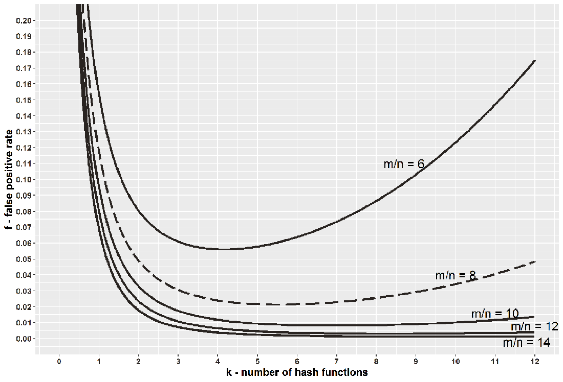
Figure 3.6 The plot relating the number of hash functions (k) and the false positive rate (f) in a Bloom filter. The graph shows the false positive rate for a fixed bits-per-element ratio (m/n), different curves corresponding to different ratios.

Starting from the top to the bottom curve, we have 6, 8, 10, 12, and 14, respectively, as choices for the bit-per-element ratio. As the ratio increases, the false positive rate drops, given the same number of hash functions. Also, the curves show the trend that increasing k up until some point (going from left to right), for a fixed m/n reduces the error, but after some point, increasing k increases the error. This two-fold effect occurs because having more hash functions allows a lookup more chances to find a 0, but sets more bits to 1 during an insert. Thus, the shape of the curves indicates that it is better to err on the larger side.

The curves are fairly smooth, and when m/n = 8 (i.e., we are willing to spend 1 byte per element), for example, if we use anywhere between 4 and 8 hash functions, the false positive rate will not go above 3%, even though the optimal choice of k is between 5 and 6.

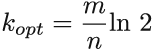
The minimum false positive rate for each curve gives us the optimal k for a particular bits-per-element ratio (which we get by doing a derivative on equation 3.1 with respect to k; see equation 3.2):

Equation 3.2

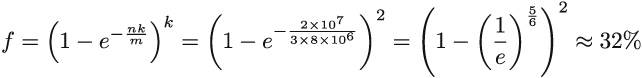
For example, when m/n = 8, k_opt = 5.545. We can use this formula to optimally configure the Bloom filter, and an interesting consequence of choosing parameters this way is that in such a Bloom filter, the false positive rate is (equation 3.3.)

Equation 3.3

Equation 3.3 is obtained by plugging equation 3.2 into equation 3.1. The constructor in our implementation takes in n and f and uses them to compute m and k, using equations 3.2 and 3.3, while making sure that k and m have to be integers. If equation 3.2 produces a noninteger, and we need to round up or down, then equation 3.3 is no longer an absolutely exact false positive rate. The only correct formula to plug into, to obtain the exact false positive rate, is equation 3.1, but even with equation 3.3, the difference produced by rounding up or down is minor. Often, it is better to choose the smaller of the two possible values of k to reduce the amount of computation.

One might find the expression (1/2)^k in equation 3.3 interesting in connection with the fact that a false positive occurs when a lookup encounters k 1s in a row. Indeed, an optimally filled Bloom filter has about a 50% probability that a random bit is 1. This is another way of saying that if your Bloom filter has too many 0s or 1s, the chances are that it is not well configured.

There are different ways to write constructors for the Bloom filter depending on what initial parameters have been provided. Usually, k is a synthetic parameter that is calculated from other, more organic requirements, such as space, number of elements, and the false positive rate. Either way, if you ever have to write different Bloom filter constructors, here are a couple of examples that show how to compute the remaining parameters.

3.4.1 Playing with Bloom filters: Mini experiments

Now that we have a basic understanding of how Bloom filters work, here are a couple of mini experiments to take our understanding to the next level.

Exercise 1

Use the provided Python implementation to create a Bloom filter where n = 10⁷ and f = 0.02. For elements, use uniform random integers (without repetition) from the range = [0,10¹²] and convert them into strings (insert them as strings). Save the inserted elements into a separate file.

Perform 10⁶ lookups that are uniformly randomly selected elements from U. Keep track of the false positive rate and verify whether it is ~2%. Measure the time required to perform the lookups. Make sure not to include the time required for the random number generation involving selecting the keys in your measurements.

Now perform 10⁶ successful lookups by uniformly randomly (without repetition) choosing from the file of inserted elements, and measure the time required to perform the lookups. Make sure you do not include the time required to read from the file or generate random numbers. What takes more time—uniform random lookups or successful lookups?

Exercise 2

Using the provided implementation, create a Bloom filter such as the one in Example 2. Now create two other filters, one in which the dataset is 100 times larger than the original one, and another one in which the dataset is 100 times smaller, leaving the same false positive rate. What do you notice about the size of the filter as the dataset size changes?

Exercise 3

In some literature, a variant of a Bloom filter is described where different hash functions have the “jurisdiction” over different parts of the Bloom filter. In other words, k hash functions split the Bloom filter into k equal-sized consecutive chunks of m/k bits, and during an insert, the i th hash function sets bits in the i th chunk. Implement this variant of the Bloom filter and check if and how this change might affect the false positive rate in comparison to the original Bloom filter.

Next, we give some instruction on how the formula for the false positive rate of the Bloom filter is derived, and how lower bounds for the space-error tradeoff in data structures work.

The next section is theoretical and intended for mathematically inclined readers. If you are more practically inclined, feel free to skip to section 3.6.

3.5 A bit of theory

First, let’s see where the main formula for the Bloom filter false positive rate (equation 3.1) comes from. For this analysis, we assume that hash functions are independent (the results of one hash function do not affect the results of any other hash function) and that each hash function maps keys uniformly randomly over the range [0 . . . m - 1].

If t is the fraction of bits in the Bloom filter that are still 0 after all n inserts took place, and k is the number of hash functions, then the probability f of a false positive is

because we need to get k 1s in order to report Present. Obtaining k 1s can also be a result of a successful lookup of an actually inserted element; however, if we consider queries to be uniformly randomly selected from a universe much larger than the dataset, then the probability of a true positive is a negligible fraction of this quantity.

The value of t is impossible to know before all inserts take place because it depends on the outcome of hashing, but we can work with probability p of a bit being equal to 0 after all inserts took place (i.e., p = Pr; a fixed bit equals 0 after n inserts).

The value of p will, in the probabilistic sense, translate to the percentage of 0s in the filter (t). We derive the value of p to be equal to the following expression:

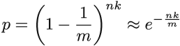
To understand why this is true, let’s start from the empty Bloom filter. Right after the first hash function h₁ has set one bit to 1, the probability that a fixed bit in the Bloom filter equals 1 is 1/m, and the probability that it equals 0 is accordingly 1 - 1/m.

After all the hashes of the first insert finished setting bits to 1, the probability that the fixed bit still equals 0 is (1-1/m)^k, and after we finished inserting the entire dataset of size n, this probability is (1-1/m)^nk. The approximation (1+1/x)^x ≈ e then further gives p ≈ e^-nk/m.

It is tempting to just replace t in the expression for the false positive rate with p, and this will give us equation 3.1. After all, p describes the expected value of a random variable denoting the percentage of 0s in the filter, but what if the actual percentage of 0s can substantially vary from its expectation?

Using Chernoff bounds—a theorem curtailing the probability of a random variable deviating substantially from its mean—we can show that the fraction of 0s in the Bloom filter is highly concentrated around its mean. The general statement of Chernoff bounds holds for random variables X that are a sum of mutually independent indicator random variables. We define a random variable X that denotes the total number of 0s in a Bloom filter X = Σ^m_i-1 X_i, where X_i = 0 if the ith bit in the Bloom filter equals 1, and X_i = 1 otherwise.

Using Chernoff bounds, we will show that the value X does not significantly deviate from its mean. In our case, X_i s is not independent, however, it is slightly negatively correlated (even better!). One bit being set to 1 slightly lowers the chance of other bits being set to 1.

The general statement of the Chernoff upper bound (we can do something similar for the lower bound), where μ is the mean of the random variable X, is as follows:

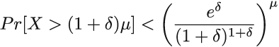
Applied to our case, μ = E[X] = mp = me^-nk/m. If we choose δ = 1 and plug into the Chernoff bound, we obtain the probability that X will deviate from its mean by more than a factor of 2:

We can safely assume that nk = θ(m), which further tells us that the probability that X deviates from the mean by more than a factor of 2 is exponentially small (< (3/4) ^θ(m)). Hence, p is a good approximation for t, the percentage of 0s in the Bloom filter, which justifies replacing t in the formula from the beginning of this section. This finalizes our derivation of equation 3.1.

3.5.1 Can we do better?

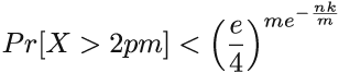
Bloom filters pack the space really well, but are there, or can there be, better data structures? In other words, for the same amount of space, can we achieve a better false positive rate? To answer this question, we need to derive a lower bound that relates the amount of space the data structure uses in bits (m) with the maximum false positive rate the data structure allows (f). Note that the lower bound is independent of any particular data structure design and tells us about the theoretical limits of any data structure—even one that has not been invented yet.

A data structure is an m-bit string and has a total of 2m distinct encodings. Each individual encoding of a data structure, in addition to reporting Present for some n elements, will also admit f(U - n) false positives, a fraction f of the rest of the universe. Of the total n + f(U - n) elements for which the data structure reports Present, we do not know which are the true positives and which are the false positives, so one encoding of the data structure serves to represent every n-sized subset we grab. There are (n + f(U - n) choose n) such sets.

In total, the data structure needs to be able to “cover” all (U choose n) n-sized subsets in the universe U. Together, these facts give us the inequality shown in figure 3.7, which describes our lower bound.

Figure 3.7 The inequality describing the space-error lower bound

Taking the logarithm on both sides, along with the fact that U >> n, and some additional algebraic manipulation, the inequality from figure 3.7 will give us

How does that compare to the false positive rate of the Bloom filter?

From equations 3.2 and 3.3, we can derive the relationship between m and the false positive rate of the Bloom filter (here we will refer to it as f_BF). We have that f_BF = (1/2)^k ≥ (1/2)^{ln 2(m/n)}. Again, taking the logarithm and doing some algebraic simplifications, we get that

.

Comparing that to the lower bound, we obtain that the Bloom filter space is log₂ e ≈ 1.44 factors away from optimal. There exist data structures that are closer to the lower bound than the Bloom filter, but some of them are very complex to understand and implement.

3.6 Bloom filter adaptations and alternatives

The basic Bloom filter data structure has been widely used in a number of systems, but Bloom filters also leave a lot to be desired, and computer scientists have developed various modified versions of Bloom filters that address some of these drawbacks. For example, the standard Bloom filter does not handle deletions. There is a version of the Bloom filter called counting Bloom filter [7] that uses counters instead of individual bits in the cells. The insert operation in the counting Bloom filter increments the respective counters, and the delete operation decrements the corresponding counters. Counting Bloom filters use more space (about four times more) and can also lead to false negatives; for example, when we repeatedly delete the same element, thereby bringing down some other element’s counters to zero.

Another issue with Bloom filters is their inability to efficiently resize. In the Bloom filter, we do not store the items or the fingerprints, so the original keys need to be brought back from the persistent storage in order to build a new Bloom filter.

Also, Bloom filters are vulnerable when the queries are not drawn uniformly randomly. Queries in real-life scenarios are rarely uniform random. Instead, many queries follow the Zipfian distribution, where a small number of elements is queried a large number of times, and a large number of elements is queried only once or twice. This pattern of queries can increase our effective false positive rate if one of our “hot” elements (i.e., the elements queried often) results in a false positive. A modification to the Bloom filter called a weighted Bloom filter [8] addresses this issue by devoting more hashes to the “hot” elements, thus reducing the chance of a false positive on those elements. There are also new adaptations of Bloom filters that are adaptive (i.e., upon the discovery of a false positive, they attempt to correct it) [9].

Another vein of research has focused on designing data structures functionally similar to the Bloom filter, but their design has been based on particular types of compact hash tables. In the next section, we cover one such interesting data structure: the quotient filter. Some of the methods employed in the next section are closely tied to designing hash tables for massive datasets, the topic of the previous chapter, but we cover it here because the main applications of quotient filters are functionally equivalent to Bloom filters, and we find uses in similar contexts.

3.7 Quotient filter

A quotient filter [10], at its simplest, is a cleverly designed hash table that uses linear probing. The difference between a quotient filter and a common hash table is that instead of storing keys into slots, as in a classic linear probing hash table, the quotient filter stores the hashes (the term fingerprint will be used interchangeably for hash). More precisely, the quotient filter stores a piece of each hash, but as we will see, it is able to reliably restore an entire hash.

On the “fidelity spectrum,” a quotient filter is somewhere between a hash table and a Bloom filter. If two distinct keys hash to the same fingerprint, the quotient filter will not be able to differentiate them the way a hash table would. But if two keys hash to different fingerprints, a quotient filter will be able to tell them apart; this is not the case with Bloom filters, where the query on a key with a unique set of k hashes might generate a false positive.

A quotient filter has similar functionality to a Bloom filter, but it has a very different design. Using longer fingerprints, quotient filters can reduce the false positive rate, but longer fingerprints might also consumes too much space.

In this section, we will see different tricks that the quotient filter employs to compactly store fingerprints. The ability to restore the full fingerprint comes in handy when we want to delete elements; yes, quotient filters can efficiently delete.

In addition, a quotient filter can resize itself, and merging two quotient filters into a larger quotient filter is a seamless, fast operation. Efficient merging, resizing, and deletions are all features that might make you want to consider using a quotient filter instead of a Bloom filter in some applications; these features are especially handy in dynamic distributed systems. Truth be told, quotient filters are a tad more complex to understand and implement than Bloom filters, but learning about them, in our opinion, is well worth your time.

In the coming sections, we will explore the design of a quotient filter, first by learning what quotienting is, then by describing how a quotient filter uses metadata bits with quotienting to save space. The best way to view a quotient filter is as a game of saving a bit here or there and employing various tricks to that end. A quotient filter is not the only data structure of this sort, but some of the tricks that you learn here can be generally useful in understanding similar data structures based on compact hash tables.

3.7.1 Quotienting

Quotienting [11] divides a hash of each item into a quotient and a remainder : in the quotient filter, the quotient is used to index into the corresponding bucket of the hash table, and the remainder is what gets stored in the corresponding slot. For example, given the h-bit hash, and table size m = 2^q, the quotient is the value determined by the leftmost q bits of the hash, and the remainder represents the remaining r = h - q bits. The example in figure 3.8 shows the fingerprint partition on a small example where m = 32 (so, q = 5) and h = 11.

Figure 3.8 Quotienting in a hash table. The item y has the hash 10100 101101; therefore, the remainder, 101101 (35), will be stored in the slot determined by a quotient, at bucket 10100 (20).

The following snippet of code shows how, once the key is hashed and the hash is stored into the variable fingerprint, the insert into the quotient filter (filter) proceeds:

h = len(fingerprint)                            ❶
 
q = log2(m)                                     ❷
 
r = h - q 
 
quotient = math.floor(fingerprint / 2**r)       ❸
 
remainder = fingerprint % 2**r                  ❹
 
filter[quotient] = remainder                    ❺

❶ Number of bits in the fingerprint

❷ Assumes the size of a hash table is a power of two

❸ q leftmost bits of the fingerprint

❹ r rightmost bits of the fingerprint

❺ The remainder gets stored in a bucket defined by the quotient (quotient does not get stored).

So far, so good. If no collisions occur (i.e., no two fingerprints ever have the same quotient), every remainder occupies its own bucket b. It is easy to reconstruct a full fingerprint by concatenating the binary representation of the bucket number b with the binary representation of the remainder stored at bucket b. Even in this small example, we managed to save q = 5 bits per slot due to quotienting.

It is important to keep in mind that in a quotient filter we can reconstruct the fingerprints, which helps with resizing and merging, but we cannot reconstruct the original elements. Again, we are somewhere between hash tables, which hold actual keys, and Bloom filters, which cannot reconstruct which element had which hashes.

However, collisions in hash tables are quite common, and quotient filters resolve collisions using a variant of linear probing. We smell trouble already because, as a consequence of linear probing, some remainders will be pushed down from their original bucket, thus losing the quotient-remainder association. To reconstruct the full fingerprint, a quotient filter uses three extra metadata bits per slot. Three bits are a small price to pay for saving ~20-30 bits per slot on a quotient in larger hash tables. In the next section we explain how metadata bits facilitate operations in the quotient filter.

3.7.2 Understanding metadata bits

Before we introduce what metadata bits stand for, a bit of terminology is needed. If you get confused by terms in this section, do not worry too much, as things should become clearer as we work on examples, see what runs and clusters are for, and see what role each metadata bit plays when resolving collisions during an insert or a lookup.

A run is a consecutive sequence of quotient filter slots occupied with remainders (i.e., fingerprints) with the same quotient (all fingerprints that collided on one particular bucket). All remainders with the same quotient are stored consecutively in the filter and in the sorted order of remainders. Due to collisions and pushing remainders down when collisions occur, a run can begin arbitrarily far from its corresponding bucket.

A cluster is a sequence of one or more runs. It is a consecutive sequence of quotient filter slots occupied by remainders, where the first remainder is stored in its originally hashed slot (we call this the anchor slot). The end of a cluster is denoted either by an empty slot or by the beginning of a new cluster.

When performing a lookup on the quotient filter, we need to decode remainders along with relevant metadata bits to retrieve the full fingerprints. The decoding always begins at the start of a containing cluster (i.e., at the anchor slot) and works downward. The three metadata bits at each slot help decode the cluster in the following manner:

• bucket_occupied—This tells us whether any key has ever hashed to the given bucket. It is 1 if some key hashed to the bucket, and 0 otherwise. This bit tells us what all the possible quotients are in the cluster.

• run_continued—This tells us whether the remainder currently stored in this slot has the same quotient as the remainder right above it. In other words, this bit is 0 if the remainder is first in its run, and 1 otherwise. This bit tells us where each run in the cluster begins and ends.

• is_shifted—This tells us whether the remainder currently stored in the slot is in its originally intended position or if it has been shifted. This bit helps us locate the beginning of the cluster. It is set to 0 only at an anchor slot, and set to 1 otherwise.

3.7.3 Inserting into a quotient filter: An example

Now, let’s work through the insertion of the elements v, w, and x, which you can see in figure 3.9. We begin with an initially empty quotient filter of 32 = 2⁵ slots, where each slot, as well as all three metadata bits, are initially set to 0:

1. Insert v: h(v) = 10001001010. The bucket determined by the quotient 10001 is previously unoccupied. We set the bucket_occupied bit to 1 and store the remainder into the slot determined by its quotient. Note that we do not need any additional action on other bits, as this item is currently both the beginning of a run and of a cluster.

2. Insert w: h(w) = 10011100111. Again, we set the bucket_occupied bit to 1 at 10011 and store the remainder into the corresponding slot as it is available, and do not modify any other bits.

3. Insert x: h(x) = 10011111111. The bucket 10011 is already occupied when we try to set the bucket to 1, so wherever we store the remainder, we will need to set run_continued of that slot to 1. The slot at the hashed bucket is taken, so wherever we store the remainder, we will need to set the is_shifted bit of that slot to 1 as well. Given that we are at the start of the cluster that has only one run (whose quotient is equal to the quotient of x), we scan downward to find the first available slot within the run at bucket 10100. We store the remainder and set the run_continued and is_shifted bits to 1.

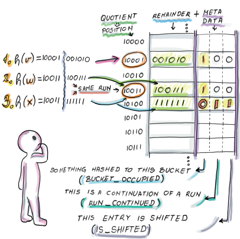
Figure 3.9 Insertion into quotient filter and metadata bits

Currently, the quotient filter has two clusters, each of which has one run. Now we insert a few more elements (follow along in figure 3.10):

1. Insert y: h(x) = 10100101101. The bucket_occupied bit at 10100 was 0, and we set it to 1 (run_continued at the final remainder’s slot will be set to 0), and the slot at the hashed bucket is taken (is_shifted at the final remainder’s slot will be set to 1). Starting from the beginning of the cluster, we look for the first place to store our new run. The first available slot is at bucket 10101, so we store the remainder and set the metadata bits accordingly.

2. Insert z: h(x) = 10100111110. The bucket_occupied bit of z’s bucket is already set to 1 (run_continued at the final slot will be 1), and the original slot is taken (is_shifted at the final slot will be 1). Starting from the start of the cluster, we decode and find where our appropriate run is. We scan down the run to the bucket 10110 to store z’s remainder and set bits accordingly.

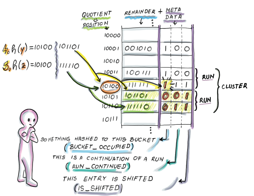
Figure 3.10 Insertion of y and z into the quotient filter.

Our insert sequence is rather simplified because the insertions arrive in the sorted order of fingerprint values. A sorted order of inserts into a quotient filter is a common scenario due to the way quotient filters are merged and resized, similar to merging sorted lists in a merge-sort, but we also need to be able to handle scenarios when inserted fingerprints arrive in the arbitrary order.

When elements are inserted out of the sorted fingerprint order, then once the correct run is found for the remainder to be inserted into it, it might push down multiple items of that run and other elements in that cluster. Consider the example of inserting an element, a, h(a) = 10100000000, into our resulting quotient filter from figure 3.10. The element would belong to the second run of the second cluster that currently occupies slots determined by buckets 10101 and 10110. An element a would move the entire run one slot below in order to get stored at slot 10101 because its remainder is the first in the ascending sorted order in that run, thus also triggering the changes in metadata bits.

Why do we need to have remainders sorted within a run (and runs among clusters)? The answer to that question will come when we talk about efficient resizing and merging.

Another important hash table-related note is that having to potentially move an entire cluster of items while inserting/deleting and decoding a whole cluster while performing lookup underlines the importance of small cluster sizes. The more empty space we leave, the smaller the probability of getting large clusters that insert, and lookup operations need to scan through and decode. Just like with common hash tables with linear probing, quotient filters work faster when the load factor is kept at 75-90% than when it is higher.

3.7.4 Python code for lookup

Now that we conceptually understand insert, let’s see how lookup works using code in Python. For the purposes of understanding the underlying logic, we will, for a moment, set aside the mechanics of compactly storing the data structure, which involves a lot of bit unpacking and shifting. Our implementation for the class Slot and the class QuotientFilter is “sparse” in that a metadata bit is an entire Boolean variable, so it takes up more than one bit of memory. Our Python code is based on the pseudocode from the original paper:

import math
 
class Slot:
    def __init__(self):
        self.remainder = 0
        self.bucket_occupied = False
        self.run_continued = False
        self.is_shifted = False
 
 
class QuotientFilter:
    def __init__(self, q, r):
        self.q = q
        self.r = r
        self.size = 2**q                                   ❶
        self.filter = [Slot() for _ in range(self.size)]
 
    def lookup(self, fingerprint):
        quotient = math.floor(fingerprint / 2**self.r)
        remainder = fingerprint % 2**self.r
        if not self.filter[quotient].bucket_occupied:
            return False                                   ❷
        b = quotient
        while(self.filter[b].is_shifted):                  ❸
            b = b - 1
        s = b
 
        while b != quotient:                               ❹
            s = s + 1
            while self.filter[s].run_continued:            ❺
                s = s + 1
            b = b + 1
 
            while not self.filter[b].bucket_occupied:      ❻
                b = b + 1
 
        while self.filter[s].remainder != remainder:       ❼
            s = s + 1
            if not self.filter[s].run_continued:
                return False
        return True

❶ Filter size

❷ No element has ever hashed to this bucket.

❸ Go up to the start of the cluster.

❹ b tracks occupied buckets, and s tracks corresponding runs.

❺ Go down the run and advance the bucket number.

❻ Skip empty buckets.

❼ Now s points to the start of the run where our element might be contained.

The lookup begins by searching for the beginning of the cluster where the item we are searching for might be contained. In other words, to find out whether an element is present, we need to decode a whole cluster.

After we find the beginning of a cluster that contains the fingerprint’s bucket, for each occupied bucket we locate its corresponding run and skip through that run until encountering the bucket that equals the quotient of our fingerprint and the start of its run (if that never happens, we return False.) Once the appropriate run is found, the lookup procedure searches inside the run for the fingerprint’s remainder.

Insertion code would also use a modified version of the lookup procedure that returns the position of the queried element, not a Boolean value. It would start by marking the appropriate bucket as occupied. Then it would use the lookup algorithm to find the appropriate location to insert the remainder, which might require shifting other remainders down until an empty slot is reached. Deletes work in a similar fashion, where they might need to move elements up to fill the hole created by the deletion, or sometimes deletes are implemented by placing a tombstone element in the said position, thereby eliminating the need for moving remainders around. If the deleted element is the only element in its run, then we also need to unmark the bucket_occupied bit. All operations in the quotient filter wrap around the table if the end of the table is reached, just like in common hash tables with linear probing.

Storing a quotient filter

An important detail in the implementation of the quotient filter, as well as many other types of compact hash tables, is how data is laid out in memory. Specifically, the slot size generally does not equal the unit sizes of addressable memory (e.g., bytes), so the byte and slot boundaries often do not align. For example, say we have a quotient filter with the remainder of length r = 7 bits, as well as three metadata bits (10 bits per slot in total). Figure 3.11 shows the memory layout of the quotient filter slots.

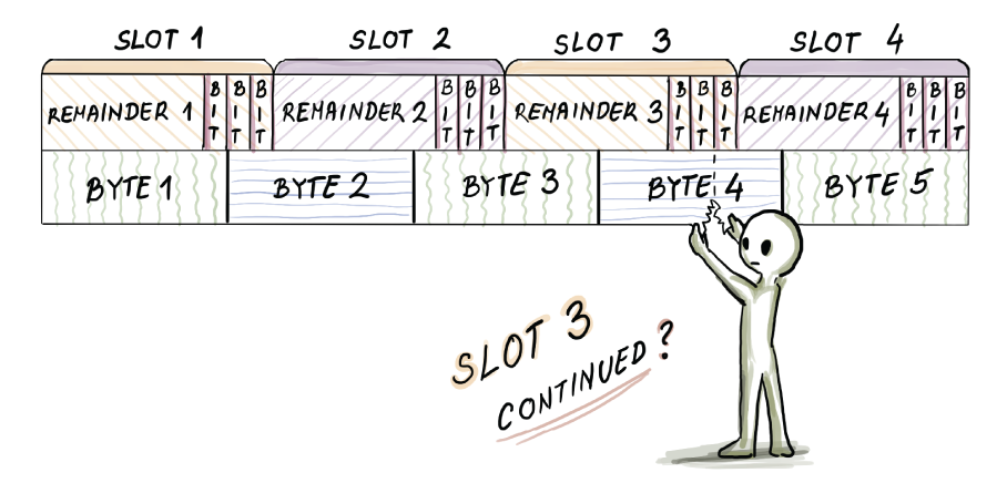
Figure 3.11 The memory layout of quotient filter slots

For example, to read slot 3’s run_continued bit, we need to access the fifth bit of byte 4. To decode a cluster, we need to do a lot of bit-shifting and bit-unpacking operations, so the quotient filter implementations (most often written in C) pay the price of small space with extra CPU cost, which, as we will see in section 3.8, impacts the in-RAM insert and lookup performance for high-load factors in a quotient filter. Unlike a Bloom filter insert that elegantly hops around setting bits to 1, a quotient filter can be very CPU-intensive. This, however, can be a good kind of a problem, as quotient filter operations move sequentially through the table, while the Bloom filter pays the price in weak spatial locality.

3.7.5 Resizing and merging

If we want to double the size of the quotient filter, it is sufficient to retrieve the fingerprint, readjust the quotient and remainder size by stealing one bit from remainder and giving it to the quotient, and insert the new fingerprint into a twice-as-large quotient filter. Generally, resizing works by traversing the quotient filter in the sorted order, decoding fingerprints as we go, and inserting them in that sorted order into the new quotient filter. The fast append operation lets us zip through the quotient filter, as inserting in the sorted order does not require a great deal of decoding and moving remainders around. A simple example of resizing a small quotient filter of size 4 is shown in figure 3.12.

Figure 3.12 Resizing a quotient filter of size 4 that contains three elements. For the sake of simplicity, we assume that no collisions occurred between those three elements and every remainder is stored in its original bucket. A fingerprint 110010 that hashed to bucket 11 (with remainder 0010) in the original quotient filter gets stored at bucket 110 of the second quotient filter (with remainder 0010), and in a 1100 bucket of the final quotient filter (with remainder 010).

Similar to how resizing is performed, we can merge two quotient filters in a fast linear-time fashion, as we would with two sorted lists in merge-sort, again enabling a fast append into a larger quotient filter.

Recall that in a Bloom filter, we cannot simply merge or resize, as we do not preserve the original elements or fingerprints. To resize a Bloom filter, we need to save the original set of keys and reload it into memory to build a new Bloom filter, which is infeasible in fast-moving streams and high-ingestion databases.

3.7.6 False positive rate and space considerations

In a quotient filter, false positives occur as a result of two distinct keys generating the same fingerprint. The analysis [12] shows that, given the table of 2^q slots and fingerprint length p = q + r, the probability of a false positive is comparable to 1/2r. The amount of space required by the quotient filter hash table is 2^q(r + 3) bits. The number of items inserted into a quotient filter is n = α 2^q where the load factor α has a significant effect on the performance of insert, lookup, and delete operations.

There also exists a variant of quotient filter that only uses two metadata bits and uses 2^q(r + 2) bits for storage, without compromising the false positive rate, but this variant substantially complicates the decoding step, making common operations too CPU-intensive on longer clusters.

Practically speaking, due to the extra space required for a linear probing table, quotient filters tend to take up slightly more space than Bloom filters for common false positive rates. For extremely low false positive rates, quotient filters are more space efficient than Bloom filters.

There are other succinct membership query data structures based on hash tables that we will not study in this chapter (e.g., the cuckoo filter [13], based on cuckoo hashing). However, we hope that the ideas you learn by studying Bloom filters and getting a taste of quotient filters, as well as their performance comparison in the next section, give you the right lens to learn about similar data structures that are out there.

3.8 Comparison between Bloom filters and quotient filters

In this section, we will summarize performance differences between Bloom filters and quotient filters. Spoiler: differences in the performance are not dramatic in either direction. However, what is more interesting are the behavioral differences between the two data structures, which stem from the way they have been designed, and that might help us understand the nature of these data structures better. Our analysis relies on the experiments previously performed in the original quotient filter paper; figure 3.13 is a rough sketch of some of their findings.

Figure 3.13 Performance comparison of Bloom filters and quotient filters on inserts, uniform random lookups, and successful lookups, respectively.

In all three graphs, the x axis represents the fraction of the data structure fullness, and the y axis represents the cumulative throughput as the data structure fills up. In this particular experiment, both data structures were given the same amount of space (2 GB) and were filled up with as many elements as possible without deteriorating the false positive rate, which was set to 1/64 for both data structures. In the case of quotient filters, performance becomes very poor after 90% occupancy, so quotient filters are only filled up until 90% full.

Uniform random inserts

As seen in figure 3.13 (left), inserts are significantly faster in quotient filters than in Bloom filters. While quotient filters at 75% occupancy have the cumulative throughput of ~3 million inserts per second, Bloom filters have the cumulative throughput of ~1.5 million inserts per second. Bloom filters need k random writes for each insert, while quotient filters usually need only 1 random write, and that is the main cause for the difference in the performance. For higher false positive rates, Bloom filters might require more hash functions, which can further degrade the insert performance. For Bloom filters, the insert performance is a flat line as the data structure fills up, while inserts slow down for the quotient filter as it fills up, as it has to decode larger clusters and drops significantly after α = 0.8.

Uniform random lookups

Uniform random lookups are slightly faster in Bloom filters than in quotient filters (figure 3.13, center); the difference becomes more striking after data structures reach 70% occupancy, and quotient filters start decoding larger clusters. Generally, uniform random lookups are faster than inserts in Bloom filters. Given a large enough universe, most uniform random lookups are unsuccessful, and when optimally filled Bloom filters reject an unsuccessful lookup after one to two probes on average; reading just one to two bits is hard to beat performance-wise.

Recall our Google WebTable query-routing example at the beginning of the chapter: unsuccessful lookup is common, so having this operation run very fast is quite favorable for Bloom filters. The uniform random lookup performance only slightly drops as the Bloom filter gets fuller, because the proportion of one bit increases, and with it, the number of bits the lookup has to check before it gives up. Quotient filters need to do a bit more work than Bloom filters by decoding a containing cluster, but this still amounts to one random read plus additional bit unpacking.

Successful lookups

Successful lookups exhibit similar performance trends to inserts (figure 3.13, right), and quotient filters again outperform Bloom filters unless for very high load factors. A Bloom filter has to check k random bits on a successful lookup (its performance is independent of how full the data structure is), while the quotient filter performance degrades with higher occupancy and larger clusters.

The experimental results do not point to a clear winner between Bloom filters and quotient filters, but their other features may point to better suitability in particular settings: a Bloom filter is simpler to implement and creates less of a burden on the CPU. A quotient filter supports deletions and works very well in distributed settings where efficient merging and resizing is important. Quotient filter variants adapted for SSD/disk also outperform Bloom filter variants intended for SSD/disk due to fast sequential merging and a small number of random reads/writes in quotient filters. To learn more about SSD/disk-adapted versions of Bloom filters and quotient filters, see a related review [14].

Summary

• Bloom filters have been widely applied in the context of distributed databases, networks, bioinformatics, and other domains where regular hash tables are too space consuming.

• Bloom filters trade accuracy for the savings in space, and there is a relationship between the space, false positive rate, number of elements, and number of hash functions in the Bloom filter.

• Bloom filters do not meet the space versus accuracy lower bound, but they are simpler to implement than more space-efficient alternatives and have been adapted over time to deal with deletes, different query distributions, and so on.

• Quotient filters are based on compact hash tables with linear probing and are functionally equivalent to Bloom filters, with the benefit of spatial locality: the ability to delete, merge, and resize efficiently.

• Quotient filters are based on the space-saving method of quotienting and extra metadata bits that allow the full fingerprint reconstruction.

• Quotient filters offer better performance than Bloom filters on uniform random inserts and successful lookups, while Bloom filters win on uniform random (unsuccessful) lookups. The performance of quotient filters is dependent on a load factor (a lower load factor is better), and the performance of Bloom filters is dependent on the number of hash functions (fewer hash functions are better).