7 Sampling from data streams

This chapter covers

• Sampling from an infinite landmark stream
• Incorporating recency by using a sliding window and how to sample from it
• Showcasing the difference between a representative and biased sampling strategy on a landmark stream with a sudden shift
• Exploring R and Python packages and libraries for writing and executing tasks on data streams

We are ready to fully appreciate sampling as a single task staged in the analysis tier. Although we have already shown that this division of the streaming data architecture is not so clear-cut, we will imagine the stream processor sampling the incoming stream in this tier. This will help to introduce the sampling algorithm without any additional complexity coming from deduplication, merging, or general preprocessing of the data. In our fingerprint-rate example, the incoming requests will first go through IP deduplication and then appear in front of the stream processor that will materialize a representative sample. The current state of the sample is then used to answer a continuous or an ad hoc query approximately but quickly. We will use our IP sampling use case to illustrate each algorithm.

Theory for sampling from a stream developed naturally from database sampling. Database sampling comes with a long and rich research and publication record, starting as early as 1986 with work by Olken and Roten [1]. One of the research directions in database sampling, online aggregation, served as an inception platform for our main topic in this chapter, sampling from data streams. We will introduce specific algorithms operating on different stream models discussed in section 6.2.

7.1 Sampling from a landmark stream

We will dip our fingers and try to “tap” into our first stream of data via sampling from a landmark stream model. This is a continuous stream of data that is not windowed. Data items arrive continuously and are operated on and disappear forever. Well, perhaps forever is too strong, since it usually moves to slow, massive, secondary memory storage. Sampling from such a stream “only” needs to somehow ensure that at every moment in the stream evolution, we are keeping a representative sample of the data seen thus far. This is an easier task compared to sampling from a windowed (sequence- or timestamp-based) data stream. Here, we don’t have to implement the logic for updating the sample once an element of the sample has exited the window (ages out). This inevitably costs time and brings us to the criterion for evaluating the “goodness” of the sampling algorithms we will present. An algorithm that answers the query well should be able to create and/or update the sample in a single pass over the elements of the stream. It should also give an approximate answer to the (continuous or ad hoc) query using the sample of size polylogarithmic in N (N being the number of stream elements seen thus far, for landmark streams). This notion of approximate must be concretized when algorithm designers want to be able to compare their solutions. The approximate answer then means that the answer should be within ε absolute/relative error of the correct answer, except for some small failure probability, δ, when it is not. We want to be ε - accurate 100 × (1 - δ) percent of the time. For windowed streams, the size of the window ω takes the role of the parameter N when we talk about polylogarithmic size. We assume that ω is too big for us to fit all tuples between t and in t - ω in memory.

7.1.1 Bernoulli sampling

Bernoulli sampling is a classical sampling strategy. (Daniel Bernoulli lived in the 18th century, when a sheet of paper with data on crop yield over time in different parts of a county was the closest concept to a database). It is also a representative sampling strategy that lived through its second spring once easily and quickly accessible data elements (the rise of database sampling) were available. The easiest way to exemplify the strategy is to imagine playing the modified game of picking petals one at a time off a flower (with the underlying audio track wondering about the existence of affection toward you). Once you ruin a perfectly fine flower, you stop with the game. What you’ve also done is sample the petals according to a degenerated version of Bernoulli sampling: you picked each petal with probability p = 1. Naturally, Bernoulli sampling of practical use will have p ∈ (0,1) with p representing the true sampling fraction for any number of elements so far encountered in the stream.

If we take our stream of deduplicated IP addresses, we can pick every 1/pth that will pass. Here lies the beauty of the simplicity of this method: at any moment we can be sure that our sample is a completely random sample of size pN, where N is the number of elements seen thus far. We can then use those to calculate an estimated number of fingerprints per IP in all the IP space.

For each arriving IP-address, we will toss a coin showing heads, with probability p, and tails with 1 - p. If we introduce the currently seen IP address each time we see heads, each IP will have p chance to be in the sample. To exemplify, with a fair coin we will, on average, take every second IP seen. Notice an inevitable feature here: although p remains constant, the size k of the sample is a binomially distributed random variable, and its expected size Np grows with N. We can now define Bernoulli sampling more formally: given a sequence of elements, e₁, e₂, e₃, ..., e_i, ..., from a landmark stream, include each element e_i of the stream with probability p ∈ (0,1) independently from any other element already passed or yet to come. Figure 7.1 illustrates this idea.

Figure 7.1 You can see how the first, fourth, and eighth element of the stream are included in the sample, since the corresponding pseudo-random value uniform on [0,1] turned out less than p = 0.3.

If you are not into nitty-gritty parts of the implementation, you now have all the necessary information about Bernoulli sampling to skip to the bottom of the next page. Naive implementation invokes a pseudo-random number generator algorithm (PRNG) for each element seen, produces a uniformly distributed random number between 0 and 1, and includes the element into a sample if the number is less than p.

Getting into the theory behind PRNGs would be a sudden and time-consuming change of context at this point. Luckily, all we need to know about PRNGs to appreciate what’s to come is that these are efficient deterministic algorithms producing a sequence of pseudo-random numbers. These numbers, if the algorithm preserves some assumptions from number theory, become indistinguishable, for practical purposes, from a sequence of real random numbers. It’s also important that they, although efficient, do cost some time, and because we are in the streaming data context, we don’t want to call them more often than necessary.

It is nice to notice that PRNGs are actually anathema to randomness (as J. von Neumann said, “Anyone who considers arithmetical methods of producing random digits is, of course, in a state of sin”), but the number theory behind them is nothing short of fascinating, so if you haven’t already, it’s in no way a waste of time to read up on them. Not the easiest, but probably the best place to do this, is chapter 3 of D. Knuth’s The Art of Computer Programming, Volume 2: Seminumerical Algorithms (1998, Addison-Wesley Professional).

To save on calls to PRNGs, our implementation will use the fact that the number of elements to skip after the last inclusion is a geometrically distributed random variable. Instead of having to do something each time a new element in the stream is seen, we’ll only operate when a new element is included in the sample. This is because we generate a “skip” of indices that we will let by each time, leading us to the next element to include.

We make use of a very general theorem from probability theory called inverse probability integral transform. (Sorry for the lofty words there!) For our case, this says that if a U is a uniformly distributed random variable on the interval (0, 1), then ∆ = [logU/log(1 – p)] gives the number of elements to skip before the next element that it is to include ([x] denotes the smallest integer less than or equal to x) if we are to include every pth one. Phew! Following is the pseudocode:

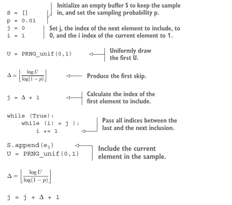
At any time t, the sample S is a Bernoulli random sample from all tuples seen so far, with inclusion probability p. As you can see from the pseudocode, we call the PRNG and log function only at times of inclusion of a new element into the sample S.

A generalized version of Bernoulli sampling uses, for each item, separate and unique inclusion probability p_i. This sampling scheme is called Poisson sampling, and inclusion of X_i is a Bernoulli trial with success probability p_i. If we have a fairly good idea about the multiplicities of X_i (i.e., in the problem of estimating the total sum of dollars from purchases, some amounts X_i show up more often than the others, say X_j), we can let them be reflected in the probabilities for inclusion. X_i with higher multiplicities will have higher p_i, while those amounts that appear only rarely will have correspondingly smaller p_i. This type of biased sampling allows for building a Horvitz-Thompson type of an estimator straightforwardly and reduces the variance of the estimate. Unfortunately, generating skips for Poisson sampling is not a trivial task.

In a distributed computing environment, in which any industrial streaming data application operates, a sampling algorithm should offer itself simply to parallelization over a number of stream (sampling) operators. The advantage of Bernoulli sampling should be obvious: sampling r substreams via Bernoulli sampling with inclusion probability p will result in a representative sample from the whole stream after the r samples are pooled at a designated master node.

The main drawback of Bernoulli sampling, as well as Poisson, is the random sample size; a landmark stream can, in theory, grow infinitely. Some attempts were made to combine Bernoulli sampling and a sample size-curtailing strategy for deleting some elements from the Bernoulli sample or using reservoir sampling once the sample size exceeds a certain threshold. Such strategies introduce some bias into the original sampling algorithm. In the case of Bernoulli sampling, the sampling strategy becomes biased, with a different bias p_i^BS - p for each element i. There is often no closed functional form of this bias, which we can use to recover p_i^BS by adding that bias to p, and hence it becomes difficult to correctly use a Horvitz-Thompson-type estimator.

7.1.2 Reservoir sampling

Reservoir sampling solves the problem of variable sample size. The algorithm was popularized among computer scientists in a 1985 paper by Vitter [2]. For any number of elements read from the stream, a sample, selected using reservoir sampling, will be uniformly distributed among all samples of size k. Proof for this claim is widely available, so we won’t show it here. Consequently, we get an SRS strategy of a fixed size k from an infinite landmark stream. Magic!

Reservoir sampling algorithm operates on a data stream as follows. First, k elements of a stream are included in the reservoir deterministically (simply append the first k elements). For every additional incoming element with index i, the probability of inclusion is for any i > k. If we are to include an element with index i, another element currently residing in the reservoir is removed uniformly at random to make place. If we add a similar shortcut that we used before to traverse elements by generating skips between those to include, instead of inspecting each, you have all that is necessary to test your understanding of the algorithm (see figure 7.1). If you are not going to implement the algorithm, but merely use it, you can still appreciate the figure. It depicts reservoir sampling for the first seven elements of the stream, using a reservoir of size k = 3.

Before we discuss the runtime of the reservoir sampling algorithm, we will describe, in detail, one possible efficient implementation of this sampling strategy. If you are not interested in this level of detail, you can safely skip the next couple of pages.

Vitter gives an efficient implementation of the algorithm using the same idea of generating the number Δ_i of skipped elements after the element with index i is included in the sample. Notice that here the number of skipped elements is equipped with an index; hence skips have a different distribution depending on how much of a data stream has been seen thus far. They change as the stream evolves. Generating such skips is more involved than for Bernoulli sampling because of the unequal (decreasing) probability of inclusion as the stream evolves. The theory behind it is not too hard and can be surveyed either in the original paper or in section 2.3 by Haas in Garofalakis, Gehrke, and Rastogi’s manuscript [3] (we will refer to this work as GGR from now on).

The method makes use of our familiar inverse probability integral transform to generate skips Δ_i for “early” i’s. For “later” i’s, the acceptance-rejection method [4] is used in combination with the squeezing argument.

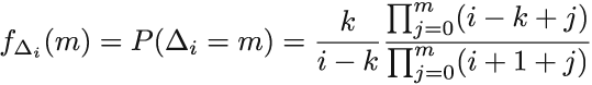
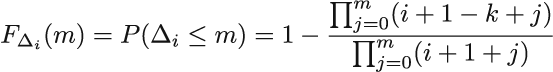
For the latter, we have to know the exact functional form of fΔ_i, which we hardly ever do. Luckily, for reservoir sampling, Viter derived the exact form for us to use. Nevertheless, we still have to evaluate it to sample with it, and that costs time. So we don’t want to call it too often. Instead, we sample using a different, easy-to-evaluate function, and use a probabilistic argument to proclaim that some of the elements sampled come from fΔ_i indirectly. That’s the high-level idea.

More specifically, we find an integrable “hat” function, h_i, over the range of fΔ_i, which is the probability mass function of Δ_i. To serve as a hat for fΔ_i, we have to have fΔ_i (x) ≤ h_i (x), meaning that the probability of Δ_i being X is always smaller than h_i(x). We then normalize h_i with the finite value α_i, which is its integral over the range of fΔ_i, to get a valid probability density function g_i(x) = h_i(x)/a_i. It makes sense to sample from the range of fΔ_i using g_i(x). We draw a random value X from g_i(x) and a uniformly distributed U from (0,1). If U ≤ fΔ_i (x)/a_ig_i (x), we take X, the current realization of X, to be a random deviate from fΔ_i; otherwise, we generate the next pair (X, U ) until the condition is fulfilled. If we abuse the notation and theory heavily, we could say that g_i(x) conditioned on U ≤ fΔ_i (x)/a_ig_i (x) is the same as fΔ_i.

We now have one more detail to cover. Remember that we want to eschew evaluating fΔ_i due to its cost. Squeezing introduces a “reversed” hat or perhaps a bowl (bathtub?) function that “props” fΔ_i “from beneath.”

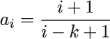
Squeezing, then, is finding a function r₁ that is inexpensive to evaluate, such that r_i (x) ≤ fΔ_i (x) for all x in the range. Then, asking U ≤ r_i (x)/a_ig_i (x) can be confirmed by the affirmative answer to U ≤ r_i (x)/a , and only in the case of a negative answer does the more expensive U ≤ r_i (x)/a_ig_i (x) have to be evaluated. We will use fΔ_i, g_i, a_i, r_i, and the cumulative distribution function G_i as Vitter derived them for us. In particular

The pseudocode shows efficient implementation of reservoir sampling. Sample size k should be set to some value. Using the example from figure 7.2, you can connect the code to your understanding of the algorithm.

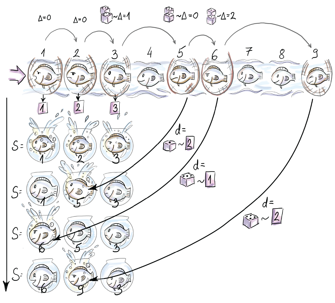
Figure 7.2 The figure shows the content of the reservoir after each of the first seven arrivals. First, three elements are included in the sample deterministically. Subsequently, e₄ is skipped (this corresponds to Δ₃, the number of elements to skip after e₃ is included, being 1). e₅ then randomly replaces e₂ in the reservoir (d = 2). The next element, e₆, is included at the random position 1 in the reservoir and replaces e₁ (notice that this means that Δ₅ was 0). Δ₆ is bigger than 0, since at least one element, e₇, is skipped.

Techniques like inverse probability integral transform, the acceptance-rejection method, and squeezing are general methods for efficient sampling from any probability distribution, so although you might need a bit of perseverance to understand how they are used, once you understand, you can tackle a wide domain of sampling tasks efficiently. Notice that the algorithm works for any number of elements coming from the stream and can be stopped at any time, resulting in a simple random sample of size k of all elements seen up to that point.

The runtime of the reservoir sampling algorithm is O (k + log n/k), so time and space requirements fit our “small space, small time constraint”—at least, in principle, since n in a landmark stream is infinite. It might be better to think about a continuous query, which uses the sample, after some specific number of elements has been seen. For the difference analysis between the runtime of the naive implementation and the one we presented with geometric jumps, see “Non-Uniform Random Variate Generation” ([chapter 12], http://www.nrbook.com/devroye/).

To understand how the reservoir sampling algorithm delivers an SRS, we will visualize a very fine balance between two sequences of probabilities. The first one is k/i := p_i the probability that ith element is included (we have referred to it as inclusion probability). The second is the probability that the ith element is not removed from the reservoir, once it is included, if we see N - i elements after it. The second probability pertains to the event when all e_j (j in index) that show up at the “door” after e_i (i in the index), fail to remove element e_i (i in the index) that sits in the reservoir.

For one specific e_j, this second probability is the sum of the probability that e_j was not selected for inclusion in the first place (e_j is skipped in this case) and the probability that, if it was selected for inclusion, it failed to remove the e_i. This sum is written as

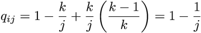
Hence, the probability that e_i is part of the reservoir after N elements are seen is

We will call this the probability of residing at N. The first part of the product (left from ×), which we denote as p_i, is inclusion probability for e_i. The second part (right from ×) is the cumulative product (we will denote it as π_iN) that captures the probability that none of the later elements remove e_i (assuming we see N elements in total). We used min to generalize the expression to accommodate the first k elements (that are included deterministically) as well. Figure 7.3 shows these two opposing forces and the resulting P_N (e_i ∈ S) for every e_i, N = 100, and k = 10.

You might remember that there aren’t many realistic data streams where we want the distant past to influence our current query to the same degree as the more recent past. This different weighting of elements based on their arrival time cannot be accomplished with reservoir sampling, so researchers try to “tilt” the balance, as shown in figure 7.3, to where more recent elements are more likely to be a part of the final sample compared to those that arrived earlier. This way the black line goes up as it approaches the current moment. This leads us to our next sampling algorithm, biased reservoir sampling.

Figure 7.3 We can see the balance between probabilities of inclusion (curved, dashed line) and probabilities of removal up to the point N = 100 (straight, dashed line) reflected in P₁₀₀(e_i ∈ S) (solid line), which is approximately constant for all elements seen so far (when the reservoir is of size 10). This means that each element, no matter when it has been seen, has the same chance of being in the sample.

7.1.3 Biased reservoir sampling

To bias the sample, we will focus on the probability of residing at N, P_N (e_i ∈ S), which determines if the element e_i at time N resides in the reservoir once it has seen N - i elements after it. We would like to be able to tilt the P_N (e_i ∈ S) from the representative equilibrium where all e_i’s have equal P_N (e_i ∈ S) (see figure 7.3). One way to do this is to assume that P_N (e_i ∈ S) decreases every time a new element arrives from the stream. We are aging out the elements nondeterminatively. This way, when e_i becomes the ever more distant past and we would rather not have it in our current reservoir, the probability of that happening becomes very small. In our IP example, you might be interested in the average number of fingerprints per IP over only the last day of traffic. In this case, you want a mechanism to govern the residing probabilities that will allow day-old elements, but no older, in the reservoir.

To achieve this, we model the probabilities of residing using some memoryless bias function f(i, N). Even though this function has two parameters, i (-th element from the stream), and N (number of elements seen thus far), it evaluates equally for all pairs (i, N) that have the same distance (N - i) between them. Therefore, P_N (e_i ∈ S) = P_N+k (e_i+k ∈ S), meaning that e_i after we have seen N elements has the same probability of residing in the reservoir as e_i+k after we have seen N + k elements. We are inquiring about elements that are at the same distance in the past from their two respective querying moments, N and N + k. The fact that we saw k new elements in the meantime leaves the two residing probabilities, P_N (e_i ∈ S) and P_N+k (e_i+k ∈ S), untouched. This is what is meant when we say memoryless. The function does not “remember” what absolute moment in time it is; it just needs to know how far in the past we are inquiring about.

You can imagine tilting P_N (e_i ∈ S) (see where the fixed N = 100 is set in figure 7.3). Notice that P_N (e_i ∈ S) stays constant for increasing i. This is what we expect from a classical reservoir sampling algorithm. Biased reservoir sampling would have P_N (e_i ∈ S) be larger as we approach the current moment and smaller toward the start of the stream (“beginning of time”).

In the original paper for biased reservoir sampling, Aggarwal [5] makes use of the memoryless exponential bias function (i, N) = e^-λ(N-i). Do you notice (N - i) in the negative exponent? When we observe the expression, we notice that the wider the gap, the bigger the exponent (and hence the smaller the negative exponent). This makes the whole expression, which is our residing probabilities, smaller P_N (e_i ∈ S). For financial data streams, or any stream for which aging elements out is beneficial, this is what we want.

The parameter λ serves as the speed of aging factor. Figure 7.4 shows P_N (e_i ∈ S) = f(i, N) for several different values of λ. We will equip you with some intuition about λ. As a part of an exercise, know that P_N (e_i ∈ S) / P_N (e_{i+ 1} ∈ S) = e^-λ. In other words, after a single new element arrives, the residing probability of the current element decreases by the factor of e^-λ. The edge case λ = 0 means “never forget,” and this, for our purpose, is a useless value of λ, but it helps to observe what happens near it. If we part from λ = 0 to the right in small, increasing steps (i.e., λ = 0, 0.001, 0.01, 0.1 . . .), e^-λ takes up values 1, 0.999, 0.99, and 0.9, in that order. Here, we see how λ governs the speed of aging; a single new element’s arrival makes the residing probability 99.9%, 99%, or 90% of what it was before the arrival. From this progression governed by λ, we can now deduce how many elements have to arrive for p_i to age out completely. If we extrapolate the reasoning, we see that e^-λ(N-i) is the inverse of the number of elements that need to arrive to decrease P_N (e_i ∈ S) by the factor of e^-1(which is multiplication by approximately 0.36; see figure 7.4). Phew! What a mouthful!

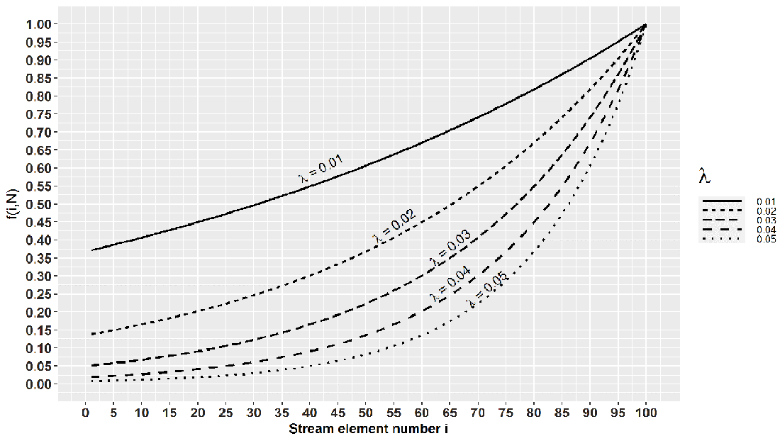
Figure 7.4 Notice that for λ = 0.01, we need 100 elements to reduce f(i,N) by the factor of 0.36, while for λ = 0.02, this number is 50. So, the higher the λ, the easier it is to forget old elements.

We will now see how one such particular λ governs the sample size too. This biased sampling scheme does not come for free, and to maintain a sample over a landmark stream, we have to meet some minimal space requirements; we have to know how the sample size grows with elements seen. Authors of the original paper denote the sample S(n) to indicate its dependency on the number of seen elements. Conveniently, they also prove that for large N (conforming with realistic streams), the size of the sample is bounded above by 1/(1 - e^-λ). From that, we bound the maximal sample size needed to achieve rates λ at which P_N (e_i ∈ S) reduces appropriately slow (or fast). That first bound can be replaced by 1/λ (using a basic calculus theorem), so all we have to facilitate is enough space for our specific, application-driven ¸ to govern our bias. If the λ we calculated in the example fits this constraint, we can use the exponential bias function with that λ. In our case, the maximum sample size is somewhere between 10⁴ and 10⁵. For the case where we can hold the entire maximal size of the sample within the (efficient) space constraints of the stream application, we can use the following simple algorithm to maintain a biased sample over any number of elements from the stream.

Assume that the jth element in the stream just arrived, and denote the occupied proportion of the reservoir by F(j) ∈ (0,1). The new element e_j is added to the reservoir deterministically. This can happen in two ways: with probability F(j), e_j substitutes a randomly chosen element from the reservoir, and with complementary probability, e_j is appended to the reservoir without resulting in any removals. The pseudocode for this version of biased reservoir sampling is shown in the code snippet on the next page. Figure 7.5 shows biased reservoir sampling for a reservoir of size k = 3(λ= 1/3) for the first seven elements of the stream.

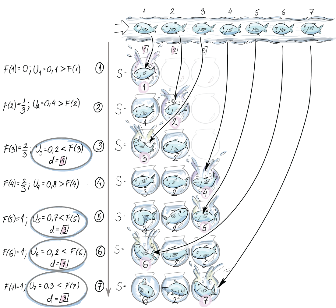
Figure 7.5 The content of the reservoir for first seven arrivals under the biased reservoir sampling strategy

e₁ is included deterministically, and e₂ is inserted without removing any existent elements from the reservoir due to the values F(2) and U₂. Since the portion of the reservoir that is occupied grows, the probability of including the next element at the expense of one existent element is higher (U₃ < F(3)); hence e₃ is saved at the first spot (d = 1). Notice that there are two possible positions for this: 1 and 2. e₄ is included at the third position without removing any elements (U₄ < F(4)). Since at this point the whole reservoir is occupied, elements e₅, e₆, and e₇ are included, all at the expense of elements saved in positions 3, 1, and 3, in that order:

S = [None] * 1/λ                    ❶
COP = 0                             ❶
i = 1                               ❶
 
while (True)
    U = PRNG_Unif(0,1)
    if U < COP
        U = PRNG_Unif(0,1)
        D = 1 + floor(k * COP * U)  ❷
        S[d] = e_i                  ❸
    else
        d = 1 + floor(k * COP)      ❹
        S[d] = e_i
        COP += 1/k                  ❹

❶ Initialize an empty buffer (reservoir) S of size k = 1/λ. Set i, the index of the current element, to 1 and the currently occupied proportion (COP) of the reservoir to 0.

❷ Draw index d between 1 and the maximal occupied index k * COP of the reservoir.

❸ Save the element e_i at that random index in the occupied part of the reservoir.

❹ Append the current element to the reservoir. In this case, we have to update the COP too.

You can go through the pseudocode and use the example from figure 7.5 to check your reasoning. Notice that once the reservoir is full, the COP is 1, and the IF-branch is always executed after that.

Exercise 2

Implement biased reservoir sampling using the provided pseudocode and the R package stream introduced in section 7.3 or using Python 3.0.

When 1/λ cannot fit into our available working buffer memory, the algorithm is modified to “slow down” the insertions by introducing a p_ins = kλ¸ probability of insertion instead of p_ins = 1. This allows us to implement the same bias in the sampling, but with a lower sample size, p_ins/λ.

This modification introduces the issue of the initial filling of the reservoir too slowly. This can lead to long waiting times to answer the sample size queries that guarantee the acceptable accuracy and precision standards. Aggarwal gives a strategy to solve this problem, so, if necessary, see his paper [5], if necessary, to implement this.

7.2 Sampling from a sliding window

We will first discuss how to sample from a sequence-based window. Here, the recency is measured in an ordinal sense as a number of arrived elements. In our IP addresses stream, the IP addresses could come at different times, but the window would be 1,000 of them long, no matter how that number spans on the time scale. We will be dealing with a sequence of windows (hence, sliding), W_j, j ≥ 1, where each indexed window entails n elements, e_j, e_j+1, e_j+2, ..., e_j+n-1. This n does not change with stream evolution as N does. The gaps between two arrivals can generally be different in absolute time units, but sequence-based windows deem these irrelevant and log the elements in consecutive integer positions. We will maintain a sample of size k from the current window. Notice that we now have to devise a strategy for updating the sample not only when we decide to insert a new element in the sample, but also every time the oldest current member of the sample exits the current window (is “aged out”). We don’t assume that the size of the window n can fit our working memory; therefore, it makes sense to sample from it.

7.2.1 Chain sampling

First, we explain how to select a random sample of size 1 from the current window and update it as the window moves. The algorithm for a random sample of size k is then just a simultaneous (parallel) execution of k instances (chains) of the strategy for keeping just one random element.

The initial phase of the algorithm that lasts n discrete time steps (length of the window) is the regular unbiased reservoir sampling, with some additional operations. Each arriving element e_i will be selected as the sample S = {e_i} with the probability i/j. This is the reservoir sampling part. The addition that handles the sliding window will pick the element that will substitute e_i when this one is aged out. We did not do this in the reservoir sampling algorithm. Hence, each time we pick a random future index, K ∈ {i + 1, i + 2, ..., i + n}, and add (K, .) to the chain. We know that the Kth element will be saved there once it enters the window. This becomes the second element of the chain. The first element (i, e_i) saves the current sample of size 1. After the whole window W₁ has been seen (n elements pass), we are in possession of a simple random sample from W₁ of size 1, because reservoir sampling guarantees that. In addition, we have the latest K, the index of the tuple that will replace it, once the sample of size 1 expires. Now, for each arriving element, i = n + 1, n + 2, ..., we have options:

• With probability 1/n, we discard the current sample, S = {e_j}, and its associated chain, saving the index K and element e_K that was supposed to inherit it once e_j expires.

• We replace it with S = {e_i}. Now e_j has to have a successor to take over after e_j expires, so we sample a random future index, K ∈ {i + 1, i + 2, ..., i + n}, and add it as the second element in the newly created chain.

• With probability (1 - 1/n), we check if i is the next replacement element to be saved in the chain (K = i?). If so, we save the ith tuple into the (last) chain element. We sample a random future index, K ∈ {i + 1, i + 2, ..., i + n}, of the element that will replace e_j once it expires and add it at the end of the chain. This is how the chain grows. In the case of = j + n, meaning e_j is leaving the window, the second element in the chain moves up, while the expired sample, S = {e_j}, is removed from the top of the chain.

These options deliver, at every discrete window-update moment i, a simple random sample of size 1 from the window W_i-n+1. Figure 7.6 shows chain sampling for first seven elements and the size of the window n = 3.

Figure 7.6 The content of the chain (list L) for the first seven elements from a sequence-based windowed stream of size n = 3

You should try to follow figure 7.6 as you read. First, the element e₁ is included deterministically. We then pick a future index, K, that will replace e₁ when e_K arrives. K seems to be 2. After we finish with the first element, the chain entails (1, e₁) and (2, .). At that moment, e₁ is the random sample of size 1. But to continue our example, element 2 arrives, and we notice that it is supposed to be saved as the successor of e₁. This is immediately done, and the chain now saves (1, e₁) and (2, e₂). These successor bookkeeping operations are done even before we decide to do them if we will sample e₂ with probability ½ (reservoir sampling) and discard e₁ and its chain altogether. We throw a die and U > 1/2 (in our case, U = 0.7); hence e₂ does not cause us to discard the existent chain. To finish dealing with e₂, its successor is drawn, and it turns out to be K = 5. Hence, the current chain is (1, e₁), (2, e₂), and (5, .). e₃ will not cause the deletion of the existent chain, either, since U₃ > 1/3. Since e₃ is nobody’s successor, it won’t be included in the chain, and we move on. At the fourth arrival, since the length of the window is n = 3, e₁ expires. We first need to update the current sample element with its successor in the chain. The role is taken over by e₂. e₄ does not cause us to discard the existent chain (U = 0.4 > 1/3), and it was not chosen as anyone’s successor, so we move on. Notice that e₄ is the first element in the second non-reservoir sampling phase. At the fifth arrival, two things happen. First, e₅ is added to its designated position in the chain, and its successor index is also included, = 7, so the chain is (2, e₂), (5, e₅), and (7, .), and it is at the peak of its length. Second, since e₂ expires, the next element in the chain, the newly added e₅, replaces it. Once we finish with e₅, we have (5, e₅) and (7, .) as the current chain and e₅ as the current sample of size 1. When e₆ arrives, we randomly choose to discard the current sample and start a new one (U = 0.2 < 1/3). The current chain, together with the sample, is discarded, and e₆ is added to the new chain and becomes the new sample. The index of its successor K is drawn, which is 8 in our example. e₇ does not cause the chain to be discarded, and since it is not anyone’s successor (it was e₅’s, but that chain was disbanded), we move past it. At each moment of the stream evolution, you can read off two important points from figure 7.5: the sample of size 1 (the shiny sparrow) and which sliding window it represents (the window it is in). The sample is always the top element of the list.

Extensively commented pseudocode for selecting a sample of size 1 using chain sampling is shown next. You can follow the code in figure 7.6 and see where the chain gets longer and when its elements are discarded to start a new chain:

L = []                            ❶
i = 1                             ❶
K = 0                             ❶
 
while i<=n                        ❷
    U = PRNG_UNIF(0,1)
    if U < 1/i                    ❸
        L.clear()                 ❹
        L.append([e_i, i])        ❺
        U = PRNG_Unif(0,1)
        K = i + floor(n*U) + 1    ❺
    else
        if i == K                 ❻
            L.append([e_i, i])
            U = PRNG_Unif(0,1)
            K = i + floor(n*U) + 1
    i+=1
 
while True                        ❼
    if (i==j+n)
        L = L.pop(1)              ❽
    U = PRNG_Unif(0,1)
    if U < 1/n
        L.clear()
        L.append 
        U = PRNG_Unif(0,1)
        K = i + floor(n*U) + 1
    else if i==K
        L.append([e_i, 1])
        U = PRNG_Unif(0,1)
        K = I + floor(n*U) + 1 
    i+=1    

❶ L is empty at the start. Set the i index of the current element to 1. Set K, the index of the future replacement element, to 0.

❷ The first phase with n elements

❸ Reservoir sampling decides to keep e_i.

❹ Remove the current sample and its chain.

❺ Add the current element e_i to the chain and determine its successor K.

❻ Reservoir sampling decides to skip e_i, so we see if it is anyone’s successor.

❼ The second phase for I = n + 1, n + 2, , , ,

❽ Remove the top element of the list because it expires from the window.

Exercise 2

Implement chain sampling for a window of length 100, sample size 1, and any N > 100.

Analysis of the space complexity for keeping k independent chains can be found in the original technical report by Babcock, Datar, and Motwani [6] or in GGR [7]. Expected memory consumption for k chains is O(k), meaning that all of them have at most a length bounded by a constant. The space complexity of the algorithm does not exceed O(k log n) with probability 1 - O(n^-c), hence by our criteria it is efficient.

Notice that each chain in the chain sampling algorithm delivers a simple random sample, at each time point, without a replacement of size 1 from the current window. Nevertheless, when we maintain k parallel chains at a time, the algorithm will deliver a simple random sample with replacement of length k, but this is not a limiting factor.

We will now present a similar algorithm for keeping a sample of size k from a timestamp-based sliding window.

7.2.2 Priority sampling

When we are dealing with timestamp-based windows, we don’t know the exact number of elements n in the window, so it is not possible to anchor our algorithm on that parameter. To keep a simple random sample (SRS) of size 1 over a timestamp-based window, we generate a priority p_t for each arriving element e_t as a uniform draw from the interval (0,1). The element with the highest priority in the window (now - ω < t < now) is our SRS of size 1. As we did with chain sampling, we will keep successors to inherit the sample once the current one exits the time-based window.

The first element e_t1 becomes our sample deterministically since there is no priority to beat (p₀ = 0). When the second element, e_t2, arrives at time t₂, we check if p_t2 > p_t1; if true, e_t2 replaces e_t1 (e_t1 is removed from memory). Otherwise, (e_t2, p_t) is saved in a linked list and as the first element of the list (the sample is saved separately and is not an element of the list). After e_t3 arrives, there are three different scenarios for ordering the priorities in memory p_t1, p_t2, and p_t3 of the newly arrived element e_t3:

1. p_t1 > p_t2 > p_t3: e_t3 is added to the tail of the list that keeps replacements in case the element e_t1, the current samples, expires. The list is ordered by descending priority and, per creation, ascending time.

2. p_t1 > p_t3 > p_t2: e_t3 is added behind e_t1, while all the elements (currently this only includes e_t2) with lower priority and (inevitably) a lower timestamp are removed from the list/memory. The list remains ordered by descending priority and, per creation, ascending time.

3. p_t3 > p_t1 > p_t2: e_t3 is added at the beginning while all other elements are removed from the list/memory. The list remains ordered by descending priority and, per creation, ascending time.

The first case adds the new element at the end of the sorted list (by priority) and keeps the whole list. The second case keeps the part of the list that has a higher priority than the new element. The third case discards the previous list and adds the new element at the top of the new one. The rest of the elements are discarded, and the new element is saved last.

The algorithm continues to update the list with each arriving element in one of the manners described. At each moment, l, on the top of the list is the element e_t, with the second highest priority among elements from the window W_l-ω, where ω is the duration of the window (l - ω < t < l). The current sample is the element with the highest priority within the time t (l - ω < t < l). The element from the top of the list substitutes the current sample and becomes the new SRS of size 1 once the current sample exits the timestamp-based window. Figure 7.7 shows the priority sampling for six elements arriving at indicated times t_is for a window size of 600 ms.

We will gradually explain what happens in figure 7.7, so it is a good idea to keep it in front of you while you read. The first element arrives at 100 ms, and p₁₀₀ is drawn to be 0.3. e₁₀₀ is set to be the current sample, while the list with the successors stays empty. At 300 ms, when e₃₀₀ arrives, its priority, p₃₀₀, is set to 0.2. Since it is smaller than the priority of the current sample, it is added in the list as the first element with its priority and time of arrival. Upon arrival, e₅₅₀ will break the priority list there, where elements that have lower priority (p < p₅₅₀ = 0.25) start. This causes e₂ to be discarded from the list. The new content of the list is e₅₅₀ only, with its priority and time of arrival. This probabilistic trimming of the list ensures the priority list doesn’t grow too large.

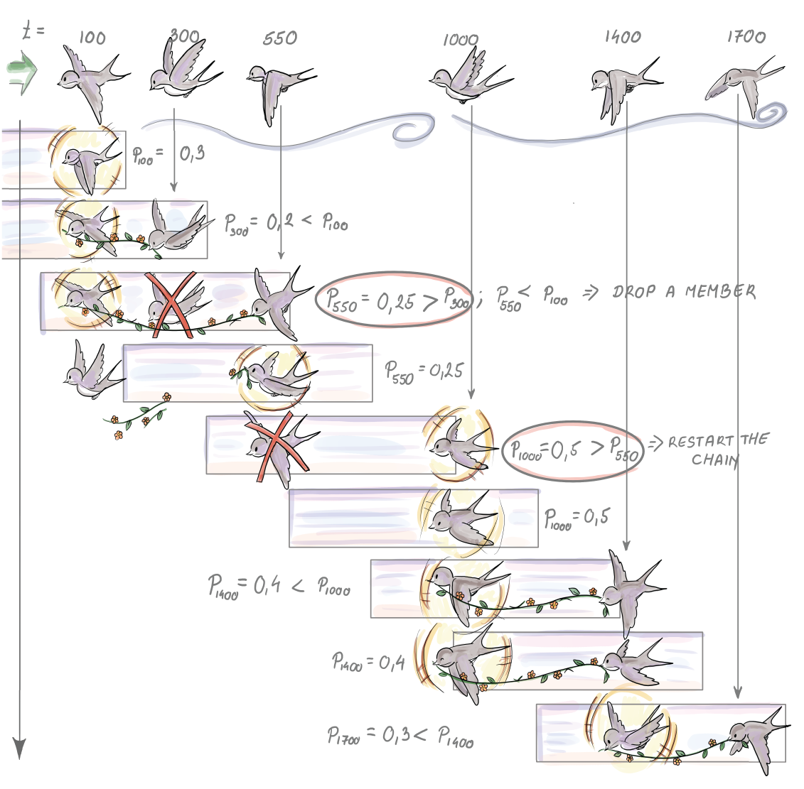
Figure 7.7 Content of the list of successors and the current sample for first six arrival times in ms for a timestamp-based window of length 600 ms

Since p₅₅₀ < p₁₀₀, the new element does not substitute the current sample; it simply becomes its new and only successor, for now. At time 700 ms, no element arrives, but since e₁₀₀ expires, we have to replace the current sample with its successor. e₅₅₀ becomes the current sample, and the list is empty. At 1,000 ms, the new element arrives. Its priority is 0.5, which is higher than the priority of the current sample. This causes e₅₅₀ to be removed and replaced by e₁₀₀₀, with its priority and time of arrival. The list with successors remains empty. e₁₄₀₀ does not have a higher priority than the current sample; hence it is added to the list as the only element so far. At 1,600 ms, the current sample e₁₀₀₀ expires and is inherited by e₁₄₀₀. The list is now empty again. When e₁₇₀₀ arrives, its priority is set to 0.3, so it is lower than p₁₄₀₀ = 0.4. Therefore, e₁₇₀₀ is added to the list as the first successor of e₁₄₀₀ once it expires.

The pseudocode and detailed comments for priority sampling of sample of size 1 are shown next. This solution will work if the inter-arrival time between any two elements of the stream is always less than ω, the window length:

L = []                                      ❶
i = 1                                       ❶
p = 0                                       ❶
 
while True:
    if len(L) == 0                          ❷
        p = PRNG_unif(0,1)
        t = ti
        L.append([eti, p, ti ])
    else if ( ti - t ≥ ω ) 
        L = L.pop(1)                        ❸
        p = PRNG_unif(0,1)
        if p ≥ L[1][2]                      ❹
            L.clear()                       ❺
            t = ti                          ❺
            L.append([eti, p, ti ])          ❺
        else                                ❻
            j = 0                   
            while p ≤ L[j][2] 
                j+=1                        ❼
                L = L[0:j]                  ❽
                L.append([eti, p , ti])      ❽
    i = i + 1                               ❾

❶ L is empty at the start. Set the i index of the current time point to 1. Set p, the priority, before any elements are seen, to 0.

❷ Handle the first element.

❸ If the current sample element expired at time t_i, remove the top-first element of the list

❹ Does the element that just arrived have a higher priority than the top-first element of the list?

❺ Empty the list and append the new element as the only member of the list. Update the time t of the current sample.

❻ We have to break the priority list somewhere beneath the top-first element.

❼ Find where to break the list and discard the “tail”.

❽ Discard the tail and append the current element in its place.

❾ Move to the next timestamp (arrival time).

The expected number of elements stored in memory for this strategy at any given time is O(ln n). To maintain a sample of size k, we can keep k lists; assign k priorities, p_t1, p_t2, p_t3, ..., p_tik, to each arriving element e_ti; and repeat the algorithm as many times with e_ti as there are lists. For this algorithm, the expected memory cost is O(k log n), while, with high probability, the cost does not exceed O(k log n) (the space complexity analysis can be found in the same references as chain sampling).

Notice that the algorithm with k lists delivering a sample of size k generates a simple random sample with replacement from a timestamp-based window.

To try out sampling from the stream in practice before we get to the actual implementation of the sampling algorithm, we first have to have a framework to handle data streams as objects. Setting up such an environment using low-level OS functions, or even using special R or Python libraries, to communicate with a streaming framework like Apache Kafka can be quite time-consuming, especially if you are just trying to quickly check if your streaming algorithm works as it is supposed to.

In the next section, we show you how to use these algorithms in the R programming language within a simple data stream framework. We will spare ourselves some groundwork with the help of the R-package stream. We give some references for a similar framework in Python.

7.3 Sampling algorithms comparison

Now that we have gotten to know a few algorithms for sampling from a stream, we will demonstrate how to use some of them in the R programming language, and in particular the R-package stream [8].This puts a data streams framework with data stream data (DSD) objects at your disposal. These can be wrappers for a real data stream, for data stored in memory or on disk, or for a generator that simulates a data stream with known properties for controlled experiments. Once we define what kind of data we will receive from the DSD object, we implement the task. In our case, this will be to maintain a random sample over the stream and use it to estimate the average value. For this we will use the class data stream task (DST).

7.3.1 Simulation setup: Algorithms and data

We will compare how well biased and unbiased sampling strategies adapt to sudden and gradual changes in the data stream. We will generate a stream with a sudden change in concept to check the robustness of the sampling algorithms with respect to this characteristic of a stream. The two algorithms operate on landmark streams, so we can talk about a random sample of size k from what we’ve seen so far. Biased reservoir sampling puts more weight on more recently seen elements, and the bias function and parameter lambda in particular determine how fast the older elements are aged out.

To simulate a sudden change in concept, we create a stream with the help of the function DSD_Gaussians(). This generator of normally distributed data creates 10⁶ Gaussian deviates. The observations from the data stream change their distribution from N(1, 1) to N(3, 1) in a single step. This means that the stream source simulates a sudden shift at one point. We split the stream in half for this purpose. We receive 500 K random values from N(1, 1), followed by 500 K random values from N(3, 1). We will try out two sample (reservoir) sizes, ∈ {10⁴, 10⁵}.

We first create the stream and then save it permanently as a csv file. This is done so that we can sample the same data with our two algorithms:

rm(list=ls())                                                                     ❶
if (!‘stream’ %in% installed.packages()) install.packages(‘stream’)               ❶
library(stream)                                                                   ❶
 
setwd(“ ”)                                                                        ❷
set.seed(1000)                                                                    ❸
stream_FirstHalf <- DSD_Gaussians(k = 1,                                          ❹
                                  d = 1, 
                                  mu=1, 
                                  sigma=c(1), 
                                  space_limit = c(0, 1)
                                  )
 
write_stream(stream_FirstHalf, "DStream.csv", n = 500000, sep = ",")              ❺
 
stream_SecondHalf <- DSD_Gaussians(k = 1,                                         ❻
                                   d = 1, 
                                   mu=3,
                                   sigma=c(1),
                                   space_limit = c(0, 1)
                                   )
 
write_stream(stream_SecondHalf, "DStream.csv", n = 500000, sep = ",", append=TRUE)❼

❶ Remove possible leftover objects in the workspace. If the package stream is not installed already, install it. Then bind the package to the workspace.

❷ Choose the path where you would like DStream.csv with the data to be saved.

❸ Set the starting position of a PRNG so that the same random data is created every time.

❹ Make a DSD object for the first half of the stream.

❺ Write 500 K elements from the DSD object to the file DStream.csv.

❻ Make a DSD object for the second half of the stream.

❼ Append 500 K elements from the DSD object to the file DStream.csv.

Implementations of the biased and unbiased reservoir sampling algorithms presented in this chapter are available in the package stream in the form of the function DSC_Sample(). In our simulations, we use two different sample sizes, 10 K and 100 K elements. We load the stream from the file using the DSD_ReadCSV class. The stream is processed in batches of 100 K elements; hence the whole stream is processed in 10 steps. In each step, we call the function update(CurrentSample, stream_file, n=100000). It expects a data stream mining task object, a DSD object, and the number of new elements to read from the stream. The paradigm behind update() is that there is a task we are executing on the stream. In our case, it is sampling from the stream. Once we read 100 K new elements from the stream, we have to adjust the current sample accordingly. Hence, calling update() makes sure our sample object has integrated the new 100 K elements into its current state. Since we call update() 10 times, we have 10 snapshots of the sample, each after additional 100 K elements have been seen. At these 10 stops, we calculate the average of the current sample and save it. We will use this later to evaluate how well the samples from biased and unbiased reservoir sampling adjust their averages to the sudden shift in the average of the stream data. We repeat this scenario for biased and unbiased reservoir sampling with sample sizes 10 K and 100 K for both. Remember that for biased reservoir sampling, λ, the speed of the aging factor is reciprocal of the sample size:

rm(list=ls()) 
if (!‘stream’ %in% installed.packages()) install.packages(‘stream’)  
  
stream_file <- DSD_ReadCSV("DStream.csv")                                 ❶
CurrentSample <- DSC_Sample(k=10000, biased=FALSE)                        ❷
 
 
MeanResults_Size10K <- NULL                                               ❸
 
for(i in seq(1,10)){
        update(CurrentSample, stream_file, 100000)                        ❹
 
        names(CurrentSample$RObj$data) <- "sample_so_far"                 ❺
 
        current_sample_avg <- mean(as.numeric(CurrentSample$RObj$data$sample_so_far))              ❻
 
        MeanResults_Size10K <- c(MeanResults_Size10K, current_sample_avg) ❼
}
 
reset_stream(stream_file, pos=1)                                          ❽
 
CurrentSample<-DSC_Sample(k=100000, biased=FALSE)
MeanResults_Size100K<-NULL
for(i in seq(1,10)){
  update(CurrentSample, stream_file, 100000)
  names(CurrentSample$RObj$data) <- "sample_so_far"    
  current_sample_avg <- mean(as.numeric(CurrentSample$RObj$data$sample_so_far))
  MeanResults_Size100K<-c(MeanResults_Size100K, current_sample_avg)
}
close_stream(stream_file)                                                 ❾

❶ Create a DSD object stream_file from our DStream.csv.

❷ Make a data mining task object that implements reservoir sampling with the option “biased” set to FALSE and the sample size to 10 K.

❸ An empty vector to save 10 averages from the 10 consecutive snapshots of the sample

❹ Update the sample with 100 K new elements.

❺ Rename the variable where the sampling object saves the sample to something more informative.

❻ Calculate the sample average.

❼ Save the sample average in the vector.

❽ Reset the stream for unbiased reservoir sampling with the sample size 100 K.

❾ Close the DSD object.

CurrentSample is an object of a DSC_Sample class, which is a subclass of the data stream task (DST) class. One can therefore use a DSC_Sample class to implement any sampling strategy as a task on a data stream. The code for the biased version of the reservoir sampling is identical, with the parameter biased set to TRUE. The λ parameter governing the bias toward new arrivals is 1/k in that case.

Figure 7.8 shows sample averages during the evolution of the stream for these two sampling strategies. We can see how the sample average changes for reservoir sampling and biased reservoir sampling and the reservoir sizes k = 10⁴, 10⁵ on a landmark stream with the sudden shift at i = 500K.

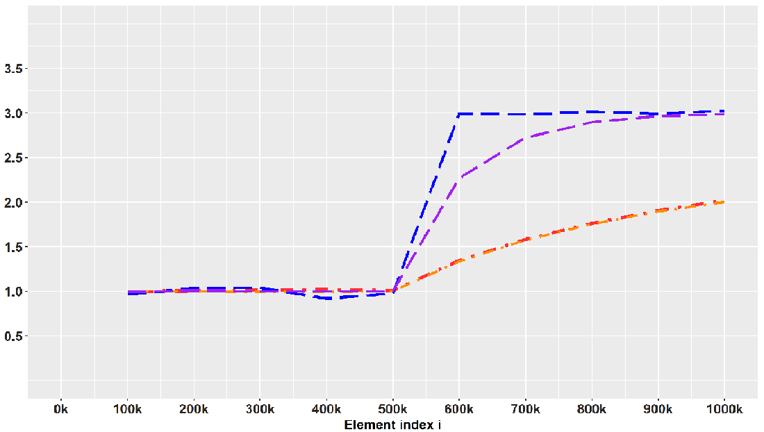
Figure 7.8 Dashed lines connect averages of samples selected using biased reservoir sampling. Upper, with λ = 10^-4, and lower, with = 10^-5, dotted and dashed lines track sample averages at every 100 K new elements for two unbiased reservoir sample sizes.

We see how biased reservoir sampling, due to uneven weighting of the recent and distant past, adapts to the sudden shift and estimates the mean very quickly and in an unbiased manner after the shift, while the unbiased reservoir sampling fails to do this. How quickly the biased strategy can detect the shift depends on the parameter λ. For λ = 10^-4 the probability of remaining in the sample decreases by e^-1 every 10,000 elements, so this λ = 10^-4 forgets faster, or has a shorter reach into the past. Therefore, the biased sample with λ = 10^-5 is slower in moving toward the current true mean. This simulation hopefully gave you some sense of the realistic conditions under which you will be sampling from a stream and the decisions you need to make given the data at hand.

For those of you who would like to try out sampling from the stream using Python, there are two options. The first is more lightweight and allows you to deploy a simple Python-based Kafka producer that reads from a .csv file of time-stamped data. The repo can be found on GitHub under MIT license (github.com/mtpatter/time-series-kafka-demo). The second is Faust, a library for building streaming applications in Python (faust.readthedocs.io/en/latest). This is a very well-documented and rich library better suited for production-level processing of data streams. If you just want to convert a .csv file of time-stamped data into a real-time stream that is useful for testing your sampling algorithm, this might be too much.

Summary

• We have gotten to know five algorithms for sampling from a data stream (three for landmark streams and two for windowed streams). Bernoulli sampling is a very simple and representative sampling algorithm, but if you want to use it, you have to think about some sample size-curbing strategy, without introducing much bias.

• Reservoir sampling solved our problem of variable sample size and delivered an SRS from elements seen at any moment. If we want to accentuate more recent elements in our sample, biased reservoir sampling is one way to go, but we need to think about our desired speed of aging and how it relates to our available space. This depends on the realistic parameters you face in your own application.

• The other option to accentuate recently arrived elements in the stream is via the sliding window. We learned how to implement chain sampling for sequence-based windows and priority sampling for time-based windows if we need to sample from that window due to its size.

• We saw how biased reservoir sampling in our simulation managed to adjust to sudden shifts in concept, while reservoir sampling was unable to react to this change and led to a biased answer of the query about the recent true average of the stream data. Remember that you do need to adjust the speed of the aging parameter so that it suits the notion of sufficient recency for your particular use case.