4 Frequency estimation and count-min sketch

This chapter covers

• Exploring practical use cases where frequency estimates arise and how count-min sketch can help
• Learning how count-min sketch works
• Exploring use cases of a sensor and an NLP app
• Learning about the error versus space tradeoff in count-min sketch
• Understanding dyadic ranges and how range queries can be solved with count-min sketch

Popularity analysis, such as producing a bestseller list on an e-commerce site, computing top-k trending queries on a search engine, or reporting frequent source-destination IP address pairs on a network, is a common problem in today’s data-intensive applications. Anomaly detection (i.e., monitoring changes in systems that are awake 24/7, such as sensor networks or surveillance cameras) falls under the same algorithmic umbrella as measuring popularity. Anomaly detection is often observed through a sudden spike in the value of a certain parameter, such as the temperature or location change in a sensor, an object appearance in the frame, or the number of units by which a company’s stock rose or fell in a given time interval.

In essence, both problems translate into measuring frequency: for each unique item key, build a data structure that can tell me how many times we encountered it. This is a problem where key-value dictionaries fit like a glove, and the amount of space taken by the dictionary is proportional not to the total sum of frequencies encountered (N), but to the total number of distinct items whose frequencies we would like to measure (n). That number, however, might be very large. This chapter deals with alternative solutions to the element-wise frequency problem when the number of distinct items is too large.

When do we encounter a large number of distinct elements? Let’s say we want to count the number of times different products were sold on an e-commerce site. If we look at the distribution of sales across products, what often happens is that there is a small number of distinct products that make up the majority of sales, and a large number of products that are sold a small number of times. This sort of distribution (also known as Zipf’s law) has been observed in many different domains. What’s tricky about measuring frequency with this type of distribution is that there is both a legitimate need to solve this problem due to large variations in frequency and a scalability issue lurking just around the corner due to many low-frequency items.

Another practical situation in which scalability issues can occur is when keys are pairs of elements, for instance, source-destination IP address pairs, or word pairs in a piece of text, where n can grow quadratically with respect to the total number of distinct IP addresses (or words), which itself might be quite high.

Also, these issues are about more than limitations on space. In this chapter, we will be interested in measuring frequency in rapid-moving streams that pose a number of difficult constraints on our choice of a data structure and an algorithm. For instance, our algorithm will be able to see each element just once (or a small, constant number of times), before we discard it and move to the next one. Solving problems such as top-k queries and heavy hitters is often impossible in this highly constrained setup. Thus, we need to resort to approximate solutions.

We will learn how a probabilistic succinct data structure, count-min sketch, can help us approximately measure frequency and solve related problems while achieving enormous space savings. We begin with the problem of heavy hitters and discuss why linear space is essential for the correct solution to this problem if we are to solve it in one pass. Then we introduce count-min sketch and its design, and we use case scenarios in the context of sensors and NLP. Toward the end of the chapter, we also discuss the error versus space tradeoff in count-min sketch and how count-min sketch can be used to answer approximate range queries.

4.1 Majority element

Let’s start with a simple problem: given an array of N elements, and provided that the array contains an element that occurs at least [N/2] + 1 times (i.e., majority element), the task is to output that element.

Exercise 1

Before moving on, try to design and implement a linear-time algorithm with constant space (other than the storage for the array) for the majority problem.

This problem can be solved using a one-pass-over-the-array algorithm [1] (also known as Boyer-More majority vote algorithm) that uses only two extra variables, as shown in the following Python code:

def majority(A):      ❶
    index = 0
    count = 1
    for i in range(len(A)):
        if A[i] == A[index]:
            count += 1
        else:
            count -= 1
        if count == 0:
            index = i
            count = 1
    return A[index]

❶ If there is a majority element in A, this function returns it.

The majority function tracks the current frontrunner for the title of majority element and resets the frontrunner once the number of occurrences (one or more) of other elements cancel it out. Assuming the provided list has a majority element, the algorithm shown will output it; otherwise, it might output an arbitrary element. If we are uncertain about whether the array has a majority element, we can perform one more sweep over the array to make sure that the returned value is indeed a majority. We show how the algorithm works on two examples—a list with a majority element and a list with an element that is almost a majority:

A = [4, 5, 5, 4, 6, 4, 4]
print(majority(A))
 
C = [3, 3, 4, 4, 4, 5]
print(majority(C))

The output is

4
5

There is also a more visual way of thinking about this problem: grab an arbitrary pair of adjacent numbers in the array that are not equal to each other, throw them out, and contract the hole created by removing the two elements. Continue grabbing pairs of different elements anywhere in the array until you are left with one distinct element, potentially its multiple copies; this element is the majority. Figure 4.1 illustrates the algorithm by showing goats vying for their position on the bridge, with the type 2 goat winning as the “majority goat.”

Figure 4.1 We find a majority element in an array by having different neighboring elements throw each other out. In this example, after we throw out (1,2), (2,5), (3,2), and then (3,2) and (4,2), we are left with the majority element 2.

Both algorithms illustrate that this problem can be solved simply in linear time with a constant memory overhead. But does this approach extend to the case of general heavy hitters?

4.1.1 General heavy hitters

The general heavy-hitters problem with a parameter k asks that the algorithm outputs all elements in the array of N items that occur more than N/k times (the majority element is the simple instance where k = 2.) There can be at most k - 1 heavy hitters, but there could also be fewer or none.

Since there can many heavy hitters, the simple application of our frontrunner algorithm implies that we should maintain many heavy-hitter candidates concurrently. To illustrate the difficulty arising from this setup, consider the following extreme case observed [2] when k = N: say we are witnessing a long data stream in which all elements discovered thus far have been distinct, and a single repetition of an element would term that element a heavy hitter. To identify a potential heavy hitter, we need to be saving each new incoming distinct element, as we do not know which one will have a repetition.

This toy example is a bit sneaky; its purpose is not to illustrate the practically occurring problem instance as much as to convince you that with larger k, the memory consumption and algorithmic complexity for solving heavy hitters grows if we want to solve the problem exactly, and that we need to turn to solving this problem approximately.

What will be approximated in heavy hitters? The (ε, k) heavy hitters ask to report all elements that occur at least N/k - εN times, that is, all the heavy hitters, and all the elements that are at most εN short of being heavy hitters for some previously set value of ε. In other words, the data structure that will store frequencies will overestimate the frequencies for some elements by the fraction ε of the total sum of frequencies N.

The data structure recording approximate frequencies that we will focus on in this chapter is count-min sketch (CMS), devised by Cormode and Muthukrishnan in 2005 [3]. Count-min sketch is like a young, up-and-coming cousin of a Bloom filter. Similar to how a Bloom filter answers membership queries approximately with less space than hash tables, the count-min sketch estimates frequencies of items in less space than a hash table or any linear-space key-value dictionary. Another important similarity is that the count-min sketch is hashing-based, so we continue in the vein of using hashing to create compact and approximate sketches of data. Next we explore how count-min sketch works.

4.2 Count-min sketch: How it works

CMS supports two main operations: update, the equivalent of an insert, and estimate, the equivalent of a lookup. For the input pair (a_t,c_t) at timeslot t, update increases the frequency of an item a_t by the quantity c_t (if, in a particular application, c_t =1, that is, the counts do not make particular sense, we can override update to only use a_t as an argument). The estimate operation returns the frequency estimate of a_t. The returned estimate can be an overestimate of the actual frequency, but never an underestimate (and that is not an accidental similarity with the Bloom filter false positives.)

Count-min sketch is represented as a matrix of integer counters with d rows and w columns (CMS[1..d][1..w]), with all counters initially set to 0 and d independent hash functions,(h₁, h₂, ..., h_d). Each hash function has the range [1..w], and the j^th hash function is dedicated to the ith row of the CMS matrix, 1 ≤ j ≤ d.

4.2.1 Update

The update operation adds another instance (or c_t instances) of an item to the dataset. Using d hash functions, update computes d hashes on a_t, and for each hash value h_j (a_t), 1 ≤ j ≤ d, the respective position in the j^th row is incremented by c_t:

CMS_UPDATE(at,ct):
    for j ← 1 to d  
        CMS[j][hj(at)] += ct

An example of how update works is shown in figure 4.2, where we begin with an empty count-min sketch and perform updates of elements x, y, and z, with quantities/ frequencies 2, 1, and 3, respectively.

Figure 4.2 Three update operations of x, y, and z performed on an initially empty 3 x 8 CMS. Computed hashes indicate which columns in the respective rows of count-min sketch need to be updated.

4.2.2 Estimate

The estimate operation reports the approximate frequency of the queried item. Just like update, estimate also computes d hashes, and it returns the minimum among d counters in d different rows, where the counter location in the j^th row is specified by hash h_j (a_t), 1 ≤ j ≤ d:

CMS_ESTIMATE(at):
    min = CMS[1][h1(at)]
    for j ← 2 to d  
        if(CMS[j][hj(at)] < min)
            min = CMS[j][hj(at)]
    return min

An example of how estimate works is shown in figure 4.3, where the estimate of element y returns the correct answer, whereas the estimate of x returns an overestimate. As we can see from the example, count-min sketch can overestimate the actual frequency due to hashes of different items colliding and contributing to counts of other elements; however, the overestimate happens only if there was a collision in each row.

Figure 4.3 Example of the estimate operation on the count-min sketch from figure 4.2. In the case of element y, whose true frequency is 1, count-min sketch reports the correct answer of 1 (the minimum of 1, 3, and 1). However, in the case of the element x, whose true frequency is 2, count-min sketch reports 3 (the minimum of 5, 3, and 5). Refer to figure 4.2 to convince yourself that during earlier update operations, y and z together incremented all the counters that are used by x, thus resulting in an overestimate for x.

4.3 Use cases

Now we move onto practical applications of count-min sketch in two different domains: a sensor smart-bed application and a natural language-processing (NLP) application.

4.3.1 Top-k restless sleepers

The quality of sleep has for a long time been linked to outcomes in an individual’s mental and physical health. However, it is only recently, with the wide access to new technologies and the ability to process enormous datasets, that we have been able to capture very detailed sleep-related data for a large number of individuals. Smart beds, for example, that come equipped with hundreds of sensors capable of recording different parameters during sleep, such as movement, pressure, temperature, and so on, can help us gain new insights into people’s sleep patterns. Based on sensor data, different bed components can adapt and modify in real time—parts of the bed can be pulled up, warmed up, cooled down, and so on.

Consider a smart-bed company that collects data from its users and stores it in one central database. There are millions of users and sensors that send out data every second; hence the amount of data is quickly becoming too large to process and analyze in a straightforward manner. Let’s assume that one smart bed features 100 sensors and that there are 10⁸ customers using this type of smart bed; then our hypothetical company collects a total of 10⁸ (customers) × 3,600 (seconds per hour) × 24 (hours per day) × 100 (sensors) = 8.6 × 10¹⁴ tuples of data daily, resulting in terabytes of storage on a daily basis. Our specific example is hypothetical, but the size of the collected data and the related problem we study are not.

With every purchase of a smart bed comes the SleepQuality mobile app that allows the beds’ users to monitor their sleep over time. One of the new app features monitors restlessness in sleepers and notifies the most restless sleepers that their sleeping patterns are out of whack in comparison to the rest of the smart sleepers. To implement this feature, the app takes into account different sensor readings and collects its findings into one point on the quality-of-sleep scale. Due to the sheer amount of data coming in, the company engineers decided to try count-min sketch to store the quantities received from users’ sensors.

As shown in figure 4.4, data arrives at a frequent rate, and at each timestep, the (user-id, amount) pair updates the count-min sketch by a given amount. In our simplified example, the keys in count-min sketch correspond to individual users; for a more refined analysis of how particular sensor readings change, the key should be a (user-id,sensor-id) pair instead.

Figure 4.4 All sleep data is sent to a central archive, but before that, it is input into count-min sketch in RAM for later analysis. The (user-id, amount) pair is used as the input for the data structure, where the frequency of user-id increases by amount. The key that is hashed is user-id.

After updating count-min sketch in this manner, we will be able to produce the approximate frequency estimate for any queried user. But in order to maintain the list of top-k restless sleepers, we will have to do a bit more than maintain the count-min sketch. Remember that the count-min sketch is just a matrix of counters, and it does not save any information on different user IDs or the ordering of relevant frequencies.

Exercise 2

Before moving onto the solution, think about what the right data structure could be to use alongside count-min sketch to store the top-k restless sleepers at each point of time, using only O(k) extra space.

One solution uses a min-heap, as shown in figure 4.5. Min-heap maintains the current k “winners” of the restlessness contest, with the possibility for updates each time a new update to the count-min sketch is received. Namely, when a new element arrives to update count-min sketch, after the update, we perform the estimate operation on this particular item. If the reported frequency is higher than the minimum item in the min-heap (easily accessible in O(1)), then the minimum of the heap is deleted and the new item is inserted. Also note that each time an update occurs for an element already in the heap, the updated frequency count needs to be reflected in the element’s position in the heap.

Figure 4.5 Using min-heap and count-min sketch together to find top-k restless sleepers. Every time the count-min sketch is updated with a (user-id, amount) pair, (100, 10) in this example, to maintain a correct list of top-k restless sleepers, we do an estimate on the frequency of the recently updated user-id. In our case, the estimate for user-id 100 will be 70. Then, if user-id is not present in the min-heap and has a higher value than the min (as it does in our example), we will extract the min and insert the new (user-id, amount) pair into the min-heap. If the pair was already present, its amount needs to be updated by deleting and reinserting the pair with the new, updated (higher) amount.

In this example, we showed that count-min sketch can be used instead of a typical key-value dictionary to preserve information on frequencies for the SleepQuality app, thereby saving a lot of space (though we have not yet analyzed the space requirements). At the same time, we used a min-heap of size O(k) to store the information on top-k restless sleepers. Min-heap maintains up-to-date estimates at each point in time, so whenever we wish to send the notification to such users, we have the information at our disposal.

4.3.2 Scaling the distributional similarity of words

The distributional similarity problem asks that, given a large text corpus, we find pairs of words that might be similar in meaning based on the contexts in which they appear (or, as the linguist John R. Firth put it, “You will know a word by a company it keeps”). For example, the words kayak and canoe will be surrounded by similar words such as water, sport, weather, river, and so on. As context for a given word, we choose the window of size k (e.g., k = 3), which includes k words before and k words after the given word in the text, or less, if we are crossing the boundary of a sentence.

One way to measure distributional similarity for a given word-context pair is using pointwise mutual information (PMI) [4]. The formula for PMI for words A and B is as follows

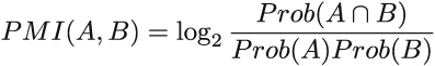
where Prob(A) denotes the probability of occurrence of A, that is, the number of occurrences of A in corpus divided by the total number of words in the corpus. It’s a fancy way of saying that PMI measures how likely A and B are to co-occur in our corpus in comparison to how often they would co-occur if they were independent. The higher the PMI, the more similar the words. Typically, to compute the PMIs for all word-context pairs or the specific word-context pairs of interest, we preprocess the corpus to produce the type of matrix shown in figure 4.6, which contains all word-context pair frequencies.

Figure 4.6 Creating a matrix M where the entry M[A][B] contains the number of times the word A appears in the context B is one way to preprocess the text corpus for computing PMI. For example, kayak appears three times in the context of water and zero times in the context of furniture. We also produce the additional count for each word (the last column of the matrix) and count for each context (the last row in the matrix), as well as for the total number of words (lower right corner).

For better association scores between words, the more text we use, the better, but with the larger corpus, even if the number of distinct words is fairly reasonable in size, the number of word-context pairs quickly gets out of hand.

For example, a research paper that measured distributional similarity using sketching techniques [5] used the Gigaword data set—a dataset obtained from English text news sources containing 9.8 GB of text and about 56 million sentences. This results in 3.35 billion word-context pair tokens and 215 million unique word-context pairs; just storing those pairs with their counts takes 4.6 GB. The solution is to transform the matrix such that the word-context pair frequencies are stored in the count-min sketch, and because the number of distinct words is not too large, we can afford to store words with their counts in their own hash table (see the last column of the matrix) and the contexts with their counts in their own hash table (see the last row of the matrix). The transformation can be seen in figure 4.7.

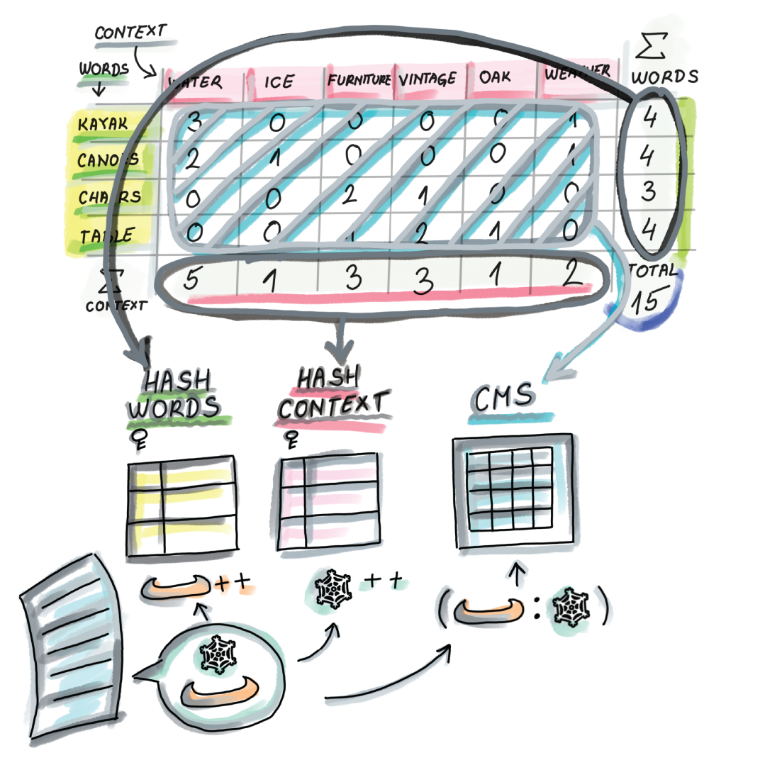
Figure 4.7 The transformation of the matrix from figure 4.6 to save space: the word-context pairs stored in the main body of the matrix are replaced by a count-min sketch that stores frequencies of word-context pairs. Because the number of distinct words (and contexts) is not that large, we can store each in their own hash table with the appropriate counts. In other words, when we encounter a new pair (word, context), we increment the count of the pair in the CMS and increment respective counts in the word hash table and the context hash table. To calculate the PMI for a word-context pair, we do an estimate query on the count-min sketch and find the appropriate counts of the word and the context in the respective hash tables.

The space savings achieved using count-min sketch in this example were over a factor of 100. The authors of this research report that a 40 MB sketch gives results comparable to other methods that compute distributional similarity using much more space. Producing this count-min sketch and the two hash tables takes just one pass over preprocessed and cleaned data, which is a big boon for the streaming datasets. We could produce top-k PMIs with an additional sweep of the data.

You might be wondering how we can configure count-min sketch (i.e., how we set its dimensions) and what the relationship is between frequency overestimate and the size of count-min sketch. Count-min sketch has two error parameters, ε and δ, and their values are used to determine the dimensions of the sketch. In the next section, we will delve into more detail about the relationship between the errors and space requirements.

4.4 Error vs. space in count-min sketch

Count-min sketch exhibits two types of errors: ε (epsilon), which regulates the band of the overestimate, and δ (delta), the failure probability. For a stream S that has come up to the timeslot t, S = (a₁, c₁), (a₂, c₂), . . . , (a_t, c_t), if we define N as the total sum of frequencies observed in the stream N = Σ^t_i = 1C_t, then the overestimate error ε can be expressed as the percentage of N by which we can overshoot the actual frequency of any item. In other words, for an element x and its true frequency f_x, count-min sketch estimates the frequency as f_est

with a probability at least 1 - δ. Usually δ is set to be small (e.g., 0.01) so that we can count on the overestimate error to stay in the promised band with high probability. There is a small probability, δ, that the overestimate in CMS can be unbounded.

Just like with the Bloom filter, we can tune CMS to be more accurate, but that will cost us space. Whatever the (ε, δ) values are that we desire for our application, to achieve the bounds stated, we need to configure the dimensions of count-min sketch to be w = e/ε and d = ln(1/δ). Hence, the space required by count-min sketch, expressed in the number of integer counters, will be (equation 4.1)

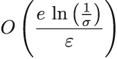
Equation 4.1

Note that CMS tends to be small, even when used on large datasets. Count-min sketch is often hailed for its space requirements—they do not depend on the dataset size—but this is only true if you desire the error to be a fixed percentage of the dataset size. For example, keeping the allowed band of error fixed at 0.3% of N will not require increasing the size of count-min sketch even if we double the value of N, but the actual absolute overestimate band will double. One could argue that with twice as large N, the application should be able to afford an overestimate error that is twice as large.

However, what leaves us wanting when it comes to count-min sketch error properties is that the overestimate error is only sensitive to the total sum of frequencies N, not to the individual element frequency. Therefore, the band of error can wildly vary if we observe it with respect to the element’s individual frequency: if the maximum overestimate is εN = 200, then we can equally expect that to be the overestimate for an element with frequency 10,000 and for an item whose frequency is 10. In the latter case, the estimate can overshoot the truth by 20 times the true frequency.

4.5 A simple implementation of count-min sketch

Now we are ready to see a bare implementation of count-min sketch. As with Bloom filters, we use the mmh3 MurmurHash wrapper for d hash functions:

import numpy as np
import mmh3
from math import log, e, ceil
 
class CountMinSketch:
    def __init__(self, eps, delta):
        self.eps = eps
        self.delta = delta
        self.w = int(ceil(e/eps))               ❶
        self.d = int(ceil(log(1. / delta)))     ❷
        self.sketch = np.zeros((self.d, self.w))
 
    def update(self, item, freq=1):
        for i in range(self.d):
            index = mmh3.hash(item, i) % self.w
            self.sketch[i][index] += freq
 
    def estimate(self, item):
        return min(self.sketch[i][mmh3.hash(item, i) % self.w] for i 
  ➥ in range(self.d))

❶ Sets width

❷ Sets depth

Try the code that shows the usage of the CountMinSketch class. Play with the updates and see how estimates change:

    cms = CountMinSketch(0.0001, 0.01)
    for i in range(100000):
        cms.update(f'{i}', 1)
    print(cms.estimate('0'))

In section 4.5.1, we provide a few exercises to test your understanding of configuring count-min sketch. Section 4.5.2 discusses the intuition behind deriving error rates in count-min sketch and is more theoretical in nature. As such, it is primarily intended for readers with an interest in the mathematical underpinnings of the data structure, and otherwise can be skipped.

4.5.1 Exercises

The following exercises are intended to check your understanding of count-min sketch, how it is configured, and how its shape and size affect the error rate.

Exercise 3

Given N = 10⁸, ε = 10^-6, and δ = 0.1, determine the error properties of the count-min sketch.

Exercise 4

Calculate the space requirements for the count-min sketch from exercise 3.

Exercise 5

Consider what happens with the size (and, more specifically, the shape) of count-min sketch if we desire a fixed absolute error (εN) while N increases. For example, say we want to keep the overestimate at 100 or less, like in exercise 3, but for an N that is twice as big.

Exercise 6

Can you design two count-min sketches that consume the same amount of space but have very different performance characteristics (with respect to their errors)? What is the practical constraint limiting the depth of the count-min sketch to low values (<30)?

Exercise 7

How would you solve the problem of the approximate k-heavy hitters mentioned in the beginning of the chapter with the help of count-min sketch? Specifically, how would you set ε to facilitate solving this problem? Recall that in approximate k-heavy hitters, we would like to report all heavy hitters and potentially those that are εN short of being heavy hitters.

4.5.2 Intuition behind the formula: Math bit

As we have observed in our simple count-min sketch implementation, to achieve the overestimate of at most εN with a probability of at least 1 - δ, the width of the count-min sketch w should be set to e/ε, and the depth of the count-min sketch d should be set to ln(1/δ). Why is w related to ε and d related to δ ?

To understand why, let us consider the process of performing updates to count-min sketch, and let us specifically focus our attention on the first row. By the time we have performed all updates to count-min sketch, the sum of the counters in the first row (and any single row) will be equal to N. Assuming that hash functions distribute updates uniformly randomly across cells, then the random variable X describing the value stored at any one fixed cell C in the first row, after all updates have been performed, has an average (or expected) value of E[X] = N/w.

This also means that when we perform an estimate for a particular item whose counter in the first row is found at cell C, other elements could contribute to its counter by no more than N/w on average. To obtain the average overestimate in one row to be no more than εN, we can set w = 1/ε. Clearly, the overestimate amount is related to the width of the data structure.

E[X] tells us about average behavior, but X can significantly deviate from its expectation: in some cells, values can be much higher than in others. We can somewhat mildly bound an overestimate in one row using Markov’s inequality, which tells us that if X is a nonnegative random variable, and c > 1, then

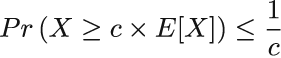
Applying Markov’s inequality to our case, we get the following:

In other words, the probability of a particular cell in the first row having the value of eN/w or larger is no greater than 1/e. But this is not good enough: to bound the probability of overestimates higher than εN, we consider all d rows. Recall that to report an overestimate of q in count-min sketch, the corresponding cells in each row need to have an overestimate of at least q. If we apply the probability arising from Markov’s inequality across all levels (note that outcomes of hash functions to different levels are mutually independent), we find that

By setting w = e/ε and d = ln(1/δ), we find that the probability that the overestimate is more than εN is at most δ.

4.6 Range queries with count-min sketch

As the final application of count-min sketch in this chapter, we’ll discuss how to report frequency estimates for ranges as opposed to single points. Range reporting has tremendous importance in databases, where the queries are often posed to reveal properties of groups and categories rather than single data points; queries such as “Give me all employees who have worked for the company between a and b years or who have salaries between x and y” naturally translate into range queries. Time series are another example of ranges; for example, “How many books were sold on Amazon.com between December 20th and January 10th of this year?”

Balanced binary search trees are good data structures for navigating ranges, as the items are in lexicographical order, so the cost of the range query, after the initial point search, is proportional to the mere cost of outputting the range query results; this is in contrast to hash tables that scatter data all over the table and where querying for a range might require a full scan of the table, even if zero items are reported. As you might imagine, that does not paint a promising picture for exploring ranges using our hash-based sketch.

The straightforward employment of count-min sketch to answer frequency estimates on ranges—by turning the range query for the range [x, y] into y - x + 1 point queries for each point along the query interval—does not give desired results. In addition to the query time growing linearly with the size of the range, the error also increases linearly with the size of the range, so instead of promising the overestimate of at most εN with a probability of at least 1 - δ, we can promise at most (y - x + 1)εN, which, for large ranges, will deem the data structure futile. For example, if we built a count-min sketch with a maximum overestimate of εN = 7, a range query of interval size 10,000 could produce an overestimate of up to 70,000.

4.6.1 Dyadic intervals

To avoid the linearly growing error, we need to find a way to decompose an arbitrary range into a small number of subranges. This way, we can obtain tighter frequency estimates by summing up frequency estimates of the smaller ranges without accumulating substantial errors [6].

The main idea is to divide a range into a small number of so-called dyadic ranges. Given a complete universe interval as U = [1, n], we define a collection of dyadic ranges at log₂ n + 1 different levels: dyadic ranges of level i, 0 ≤ i ≤ log₂ n are of length 2ⁱ and can be expressed as [j2ⁱ + 1, (j + 1)2ⁱ], where 0 ≤ j ≤ n/2ⁱ -1 (see figure 4.8 for a set of dyadic ranges for universe interval U = [1,16]).

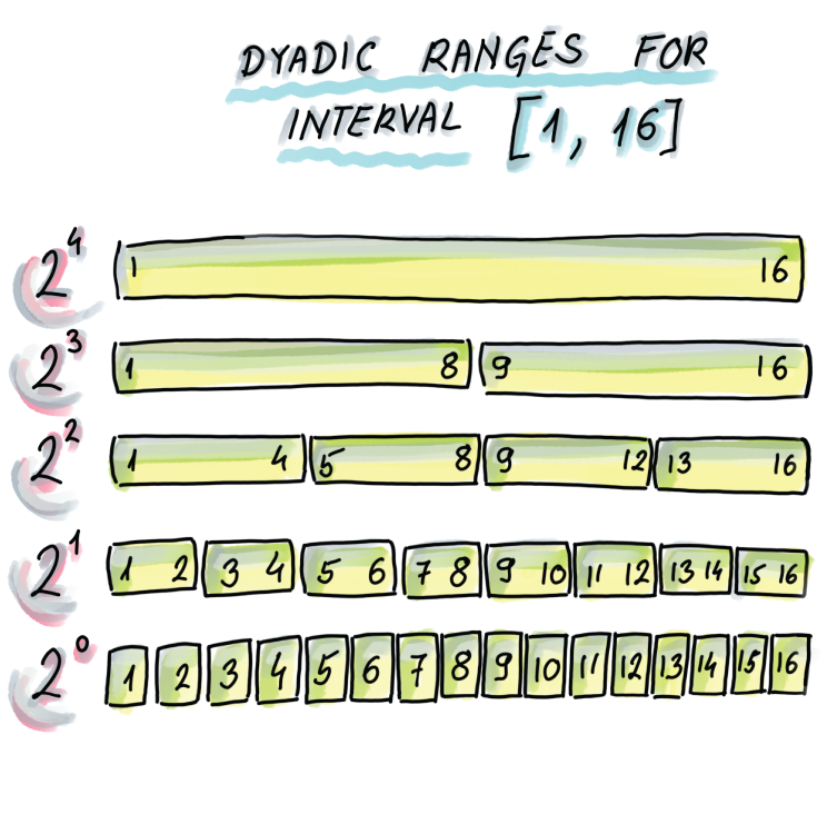
Figure 4.8 Dyadic ranges for the interval [1, 16]. Dyadic ranges of level 0 are the bottom, with ranges of size 1; then the ranges of level 1 are the level above, with the ranges of size 2; and general dyadic ranges at level i are of size 2ⁱ. Dyadic ranges across different levels are mutually aligned.

The interesting property of dyadic ranges is that any arbitrary range can be decomposed into at most 2logU dyadic ranges. Later in this section, we will show the Python code that can decompose an arbitrary range into a set of dyadic ranges, but first, as an example, consider our small universe from figure 4.8, and see a few examples of separating ranges into the smallest set of dyadic ranges:

• Range [5,14] can be separated into three dyadic ranges: [5,8], [9,12], [13,14]

• Range [2,16] can be separated into four dyadic ranges: [2,2], [3,4], [5,8], [9,16]

• Range [9,13] can be separated into two dyadic ranges: [9,13], [13,13]

To report the range frequency as the sum of frequencies of dyadic ranges, as updates take place, we need to maintain the frequency information for each dyadic range. To that end, we can use one count-min sketch to serve all updates for dyadic ranges of one level (dyadic ranges of the same size) for a total of O(log n) count-min sketches. Next, we describe this scheme in more detail.

4.6.2 Update phase

Considering that our unit elements are now dyadic ranges, we need to convert an update of a single element arriving to our system to an update of each dyadic range the element is contained in. For example, when updating the frequency of element 5 in our example universe [1,16], we will update the frequency of the following dyadic ranges: [5], [5,6], [5,8], [1,8], and [1,16]. Ranges can be hashed just like regular elements, so there is no obstacle in a dyadic range of the format [l,r] being treated as one element.

We accomplish this using O(log n) count-min sketches by building one count-min sketch for each level of dyadic range; the elements to be updated/estimated in the count-min sketch on the level i will be the dyadic ranges of that level. Figure 4.9 shows how the update of a new element takes place: an arriving new element will be updated in each count-min sketch by updating its containing range in the respective CMS.

Figure 4.9 An update of one element is transformed into one update per level. For example, if we update 5, we effectively update [1,16] in CMS1, [1,8] in CMS2, [5,8] in CMS3, [5,6] in CMS4, and [5] in CMS5. Instead of updating an element, we are updating a corresponding range to which the element belongs in the relevant CMS.

4.6.3 Estimate phase

Now we are ready to perform an estimate on a particular range using dyadic ranges. First we divide the query range into its own set of dyadic ranges. For each dyadic range, we perform an estimate in the CMS that resides on its level (there can be at most two dyadic ranges on the same level per query.) The final result comes from summing up all the estimates. Figure 4.10 shows how we can do the range estimate for [3,13], whose frequency estimate we obtain by estimating the following dyadic ranges in the respective CMSs and summing them: [3,4], [5,8], [9,12], and [13].

Figure 4.10 In this example, the query range [3,13] is separated into [3,4]∪[5,8]∪[9,12]∪[13], and we will obtain the frequency estimate for [3,13] by obtaining the frequency estimates for the mentioned ranges and summing them.

It helps to know that every range can be partitioned into at most 2log n dyadic ranges (at most two per level). Both for the update and for the estimate, the runtime is logarithmic and the error grows only logarithmically. We can make the error the same as in the original single-count min sketch by making the individual CMSs in this scheme, by a logarithmic factor, wider, so that the logarithms cancel out.

4.6.4 Computing dyadic intervals

The Python code shown gives a decomposition of I into dyadic intervals, where we are given the large universe U and a range 1 ⊆ U. First, we build a full binary search tree based on the universe interval, similar to figure 4.8, where each level corresponds to a level of dyadic ranges, and each node corresponds to a unique dyadic range. For instance, the root node represents the range [1,n], its left child represents the range [1,n/2], its right child represents the range [n/2 + 1,n], and so on. The leaves represent the ranges of size 1, and there are n of them. We construct such a tree from the universe interval:

from collections import deque
 
class Node:                             ❶
    def __init__(self, lower, upper):
        self.data = (lower, upper)
        self.left = None
        self.right = None
        self.marked = False
 
def intervalToBST(left, right):         ❷
    if left == right:
        root = Node(left, right)
        return root
    if abs(right - left) >= 1:
        root = Node(left, right)
        mid = int((left + right) / 2)
        root.left = intervalToBST(left, mid)
        root.right = intervalToBST(mid + 1, right)
        return root

❶ Each node represents a dyadic range.

❷ Transforms the interval [left, right] into a binary search tree

Given a particular range, we now compute a set of its dyadic ranges using the binary search tree we constructed. We also use a marked attribute at each node. The nodes that end up having a marked attribute of True will be the nodes that represent the dyadic subranges of the query range. The algorithm works by first marking each leaf that is a subrange of the interval I. Then it works in a level-by-level fashion going up the tree, and if a node has both children marked, we mark that node and unmark the children. The algorithm stops after we have processed the root node.

Consider a simple interval, I = [1,5], in a universe interval, U = [1,16]. On the bottom level of the tree, we mark the nodes representing the following intervals: [1,1], [2,2], [3,3], [4,4], and [5,5]. Then we go one level up and find that for node [1,2], both of its children, [1,1] and [2,2], are marked, so we mark [1,2] (and unmark [1,1] and [2,2]). Similarly, we mark [3,4] because [3,3] and [4,4] are marked and unmark [3,3] and [4,4]. On the third level from the bottom, we mark [1,4] because [1,2] and [3,4] are marked and unmark [1,2] and [3,4]. We also process nodes from all other levels all the way to the root, but we do not encounter any more nodes with both children marked as True. Therefore, there are two marked nodes left, and those correspond to the subranges [1,4] and [5,5], and we report them as our dyadic ranges. This functionality is illustrated in the following code:

def markNodes(root, lower, upper):
    if root is None:                                       ❶
        return
    queue = [root]
    stack = deque()
    while(len(queue) > 0):
        stack.append(queue[0])
        node = queue.pop(0)
        if node.left is not None:
            queue.append(node.left)
        if node.right is not None:
            queue.append(node.right)
 
    while(len(stack) > 0):                                 ❷
        i = stack.pop()
        if i.data[0] >= lower and i.data[1] <= upper and 
  ➥ i.left is None and i.right is None:                   ❸
            i.marked = True
 
        if i.left is not None and i.right is not None:
            if i.left.marked and i.right.marked:           ❹
                i.left.marked = False
                i.right.marked = False
                i.marked = True
 
def inorderMarked(root):                                   ❺
    if root is None:
        return
    inorderMarked(root.left)
    if root.marked:
        print(root.data)
    inorderMarked(root.right)

❶ First traverse the nodes in a level-by-level order (BFS traversal).

❷ The stack stores nodes in a level-by-level order, starting from the leaves.

❸ Each leaf inside the interval is marked.

❹ Mark internal nodes whose two children were both marked, and unmark the children.

❺ Print dyadic ranges.

Here is how this implementation works on an example of universe interval U = [1,16] and interval I = [3,13]:

k = 4
root = intervalToBST(1, 2**k)
markNodes(root, 3, 13)
inorderMarked(root)

The output dyadic intervals are

(3, 4)
(5, 8)
(9, 12)
(13, 13)

The time to complete the algorithm in the worst case is the time asymptotically required by the breadth-first search algorithm on the universe tree, hence O(n).

Summary

• Frequency estimation problems commonly arise in the analysis of big data, especially in sets that have many occurrences of very few items and a small number of occurrences of many items. Even though in the standard RAM setting frequency estimation can be simply solved in linear space, solving this problem becomes very challenging in the context of streaming data where we are allowed only one pass over the data and sublinear space.

• Count-min sketch is well suited to solve the approximate heavy-hitters problem, as well as many other problems in sensor and NLP domains.

• Count-min sketch is very space efficient and has two error parameters, ε (controlling band of overestimate) and δ (controlling the failure probability) that are tunable and determine the sketch’s dimensions. If the allowed band of overestimate error is kept as a fixed percentage of the total quantity of data N, then the amount of space in count-min sketch is independent of the dataset size.

• It is possible to do fairly accurate frequency estimates for range queries using count-min sketch by decomposing a range into a set of dyadic ranges and using O(log n) count-min sketches.