
CHAPTER TWENTY
Minimum Spanning Trees
GRAPH MODELS WHERE we associate weights or costs with each edge are called for in many applications. In an airline map where edges represent flight routes, these weights might represent distances or fares. In an electric circuit where edges represent wires, the weights might represent the length of the wire, its cost, or the time that it takes a signal to propagate through it. In a job-scheduling problem, weights might represent time or the cost of performing tasks or of waiting for tasks to be performed.
Questions that entail cost minimization naturally arise for such situations. We examine algorithms for two such problems: (i) find the lowest-cost way to connect all of the points, and (ii) find the lowest-cost path between two given points. The first type of algorithm, which is useful for undirected graphs that represent objects such as electric circuits, finds a minimum spanning tree; it is the subject of this chapter. The second type of algorithm, which is useful for digraphs that represent objects such as an airline route map, finds the shortest paths; it is the subject of Chapter 21. These algorithms have broad applicability beyond circuit and map applications, extending to a variety of problems that arise on weighted graphs.
When we study algorithms that process weighted graphs, our intuition is often supported by thinking of the weights as distances: We speak of “the vertex closest to x,” and so forth. Indeed, the term “shortest path” embraces this bias. Despite numerous applications where we actually do work with distance and despite the benefits of geometric intuition in understanding the basic algorithms, it is important to remember that the weights do not need to be proportional to a distance at all; they might represent time or cost or an entirely different variable. Indeed, as we see in Chapter 21, weights in shortest-paths problems can even be negative.
To appeal to intuition in describing algorithms and examples while still retaining general applicability, we use ambiguous terminology where we refer interchangeably to edge lengths and weights. When we refer to a “short” edge, we mean a “low-weight” edge, and so forth. For most of the examples in this chapter, we use weights that are proportional to the distances between the vertices, as shown in Figure 20.1. Such graphs are more convenient for examples, because we do not need to carry the edge labels and can still tell at a glance that longer edges have weights higher than those of shorter edges. When the weights do represent distances, we can consider algorithms that gain efficiency by taking into account geometric properties (Sections 20.7 and 21.5). With that exception, the algorithms that we consider simply process the edges and do not take advantage of any implied geometric information (see Figure 20.2).
The problem of finding the minimum spanning tree of an arbitrary weighted undirected graph has numerous important applications, and algorithms to solve it have been known since at least the 1920s; but the efficiency of implementations varies widely, and researchers still seek better methods. In this section, we examine three classical algorithms that are easily understood at a conceptual level; in Sections 20.3 through 20.5, we examine implementations of each in detail; and in Section 20.6, we consider comparisons of and improvements on these basic approaches.
Definition 20.1 A minimum spanning tree (MST) of a weighted graph is a spanning tree whose weight (the sum of the weights of its edges) is no larger than the weight of any other spanning tree.
If the edge weights are all positive, it suffices to define the MST as the set of edges with minimal total weight that connects all the vertices, as such a set of edges must form a spanning tree. The spanning-tree condition in the definition is included so that it applies for graphs that may have negative edge weights (see Exercises 20.2 and 20.3).
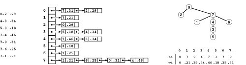
Figure 20.1 A weighted undirected graph and its MST
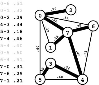
A weighted undirected graph is a set of weighted edges. The MST is a set of edges of minimal total weight that connects the vertices (black in the edge list, thick edges in the graph drawing). In this particular graph, the weights are proportional to the distances between the vertices, but the basic algorithms that we consider are appropriate for general graphs and make no assumptions about the weights (see Figure 20.2).
If edges can have equal weights, the minimum spanning tree may not be unique. For example, Figure 20.2 shows a graph that has two different MSTs. The possibility of equal weights also complicates the descriptions and correctness proofs of some of our algorithms. We have to consider equal weights carefully, because they are not unusual in applications and we want to know that our algorithms operate correctly when they are present.
Not only might there be more than one MST, but also the nomenclature does not capture precisely the concept that we are minimizing the weight rather than the tree itself. The proper adjective to describe a specific tree is minimal (one having the smallest weight). For these reasons, many authors use more accurate terms like minimal spanning tree or minimum-weight spanning tree. The abbreviation MST, which we shall use most often, is universally understood to capture the basic concept.
Still, to avoid confusion when describing algorithms for networks that may have edges with equal weights, we do take care to be precise to use the term “minimal” to refer to “an edge of minimum weight” (among all edges in some specified set) and “maximal” to refer to “an edge of maximum weight.” That is, if edge weights are distinct, a minimal edge is the shortest edge (and is the only minimal edge); but if there is more than one edge of minimum weight, any one of them might be a minimal edge.
We work exclusively with undirected graphs in this chapter. The problem of finding a minimum-weight directed spanning tree in a di-graph is different, and is more difficult.
Several classical algorithms have been developed for the MST problem. These methods are among the oldest and most well-known algorithms in this book. As we have seen before, the classical methods provide a general approach, but modern algorithms and data structures can give us compact and efficient implementations. Indeed, these implementations provide a compelling example of the effectiveness of careful ADT design and proper choice of fundamental ADT data structure and algorithm implementations in solving increasingly diffi-cult algorithmic problems.
Exercises
20.1 Assume that the weights in a graph are positive. Prove that you can rescale them by adding a constant to all of them or by multiplying them all by a constant without affecting the MSTs, provided only that the rescaled weights are positive.
Figure 20.2 Arbitrary weights
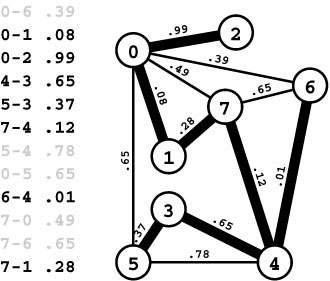
In this example, the edge weights are arbitrary and do not relate to the geometry of the drawn graph representation at all. This example also illustrates that the MST is not necessarily unique if edge weights may be equal: we get one MST by including 3-4 (shown) and a different MST by including 0-5 instead (although 7-6, which has the same weight as those two edges, is not in any MST).
20.2 Show that, if edge weights are positive, a set of edges that connects all the vertices whose weights sum to a quantity no larger than the sum of the weights of any other set of edges that connects all the vertices is an MST.
20.3 Show that the property stated in Exercise 20.2 holds for graphs with negative weights, provided that there are no cycles whose edges all have non-positive weights.
• 20.4 How would you find a maximum spanning tree of a weighted graph?
• 20.5 Show that if a graph’s edges all have distinct weights, the MST is unique.
• 20.6 Consider the assertion that a graph has a unique MST only if its edge weights are distinct. Give a proof or a counterexample.
• 20.7 Assume that a graph has t < V edges with equal weights and that all other weights are distinct. Give upper and lower bounds on the number of different MSTs that the graph might have.
20.1 Representations
In this chapter, we concentrate on weighted undirected graphs—the most natural setting for MST problems. Perhaps the simplest way to begin is to extend the basic graph representations from Chapter 17 to represent weighted graphs as follows: In the adjacency-matrix representation, the matrix can contain edge weights rather than Boolean values; in the adjacency-lists representation, we can add a field for the weights to the list elements that represent edges. This classic approach is appealing in its simplicity, but we will use a different method that is not much more complicated and will make our programs useful in more general settings. Comparative performance characteristics of the two approaches are briefly treated later in this section.
To address the issues raised when we shift from graphs where our only interest is in the presence or absence of edges to graphs where we are interested in information associated with edges, it is useful to imagine scenarios where vertices and edges are objects of unknown complexity, perhaps part of a a huge client data base that is built and maintained by some other application. For example, we might like to view streets, roads, and highways in a map data base as abstract edges with their lengths as weights, but, in the data base, a road’s entry might carry a substantial amount of other information such as its name and type, a detailed description of its physical properties, how much traffic is currently using it, and so forth. Now, a client program
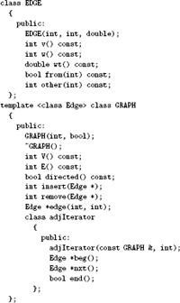
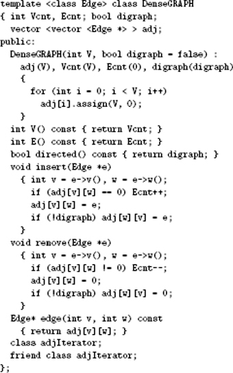
Program 20.1 ADT interface for graphs with weighted edges
This code defines an interface for graphs with weights and other information associated with edges. It consists of an EDGE ADT interface and a templatized GRAPH interface that may be used for any EDGE implementation. GRAPH implementations manipulate edge pointers (provided by clients with insert), not edges. The edge class also includes member functions that give information about the orientation of the edge: Either e->from(v) is true, e->v() is v and e->other(v) is e->w(); or e->from(v) is false, e->w() is v and e->other(v) is e->v().
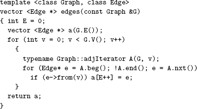
Program 20.2 Example of a graph-processing client function
This function illustrates the use of our weighted-graph interface in Program 20.1. For any implementation of the interface, edges returns a vector containing pointers to all the graph’s edges. As in Chapters 17 through 19, we generally use the iterator functions only in the manner illustrated here.
could extract the information that it needs, build a graph, process it, and then interpret the results in the context of the data base, but that might be a difficult and costly process. In particular, it amounts to (at least) making a copy of the graph.
A better alternative is for the client to define an Edge data type and for our implementations to manipulate pointers to edges. Program 20.1 shows the details of the EDGE, GRAPH, and iterator ADTs that we use to support this approach. Clients can easily meet our minimal requirements for the EDGE data type while retaining the flexibility to define application-specific data types for use in other contexts. Our implementations can manipulate edge pointers and use the interface to extract the information they need from EDGEs without regard to how they are represented. Program 20.2 is an example of a client program that uses this interface.
For testing algorithms and basic applications, we use a class EDGE, which has two ints and a double as private data members that are initialized from constructor arguments and are the return values of the v(), w(), and wt() member functions, respectively (see Exercise 20.8). To avoid proliferation of simple types, we use edge weights of type double throughout this chapter and Chapter 21. In our examples, we use edge weights that are real numbers between 0 and 1. This decision does not conflict with various alternatives that we might need in applications, because we can explicitly or implicitly rescale the weights to fit this model (see Exercises 20.1 and 20.10). For example, if the weights are positive integers less than a known maximum value, we can divide them all by the maximum value to convert them to real numbers between 0 and 1.
Program 20.3 Weighted-graph class (adjacency matrix)
For dense weighted graphs, we use a matrix of pointers to Edges, witha pointer to the edge v-w in row v and column w. For undirected graphs, we put another pointer to the edge in row w and column v. The null pointer indicates the absence of an edge; when we remove an edge, we remove our pointer to it. This implementation does not check for parallel edges, but clients could use edge to do so.
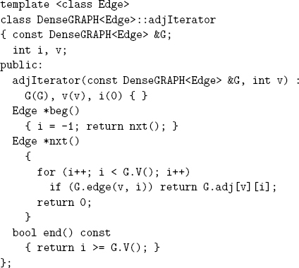
Program 20.4 Iterator class for adjacency-matrix representation
This code is a straighforward adaptation of Program 17.8 to return edge pointers.
If we wanted to do so, we could build a more general ADT interface and use any data type for edge weights that supports addition, subtraction, and comparisons, since we do little more with the weights than to accumulate sums and make decisions based on their values. In Chapter 22, our algorithms are concerned with comparing linear combinations of edge weights, and the running time of some algorithms depends on arithmetic properties of the weights, so we switch to integer weights to allow us to more easily analyze the algorithms.
Programs 20.3 and 20.4 implement the weighted-graph ADT of Program 20.1 with an adjacency-matrix representation. As before, inserting an edge into an undirected graph amounts to storing a pointer to it in two places in the matrix—one for each orientation of the edge. As is true of algorithms that use the adjacency-matrix representation for unweighted graphs, the running time of any algorithm that uses this representation is proportional to V2 (to initialize the matrix) or higher.
With this representation, we test for the existence of an edge v-w by testing whether the pointer in row v and column w is null. In some situations, we could avoid such tests by using sentinel values for the weights, but we avoid the use of sentinel values in our implementations.
Program 20.5 gives the implementation details of the weighted-graph ADT that uses edge pointers for an adjacency-lists representation. A vertex-indexed vector associates each vertex with a linked list of that vertex’s incident edges. Each list node contains a pointer to an edge. As with the adjacency matrix, we could, if desired, save space by putting just the destination vertex and the weight in the list nodes (leaving the source vertex implicit) at the cost of a more complicated iterator (see Exercises 20.11 and 20.14).
At this point, it is worthwhile to compare these representations with the simple representations that were mentioned at the beginning of this section (see Exercises 20.11 and 20.12). If we are building a graph from scratch, using pointers certainly requires more space. Not only do we need space for the pointers, but also we need space for the indices (vertex names), which are implicit in the simple representations. To use edge pointers in the adjacency-matrix representation, we need extra space for V2 edge pointers and E pairs of indices. Similarly, to use edge pointers in the adjacency-list representation we need extra space for E edge pointers and E indices.
On the other hand, the use of edge pointers is likely to lead to faster code, because the compiled client code will follow one pointer to get direct access to an edge’s weight, in contrast to the simple representation, where an Edge needs to be constructed and its fields accessed. If the space cost is prohibitive, using the minimal representations (and perhaps streamlining the iterators to save time) certainly is a reasonable alternative; otherwise, the flexibility afforded by the pointers is probably worth the space.
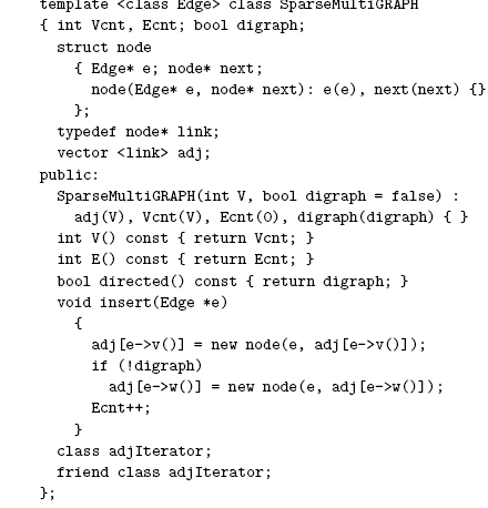
Program 20.5 Weighted-graph class (adjacency lists)
This implementation of the interface in Program 20.1 is based on adjacency lists and is therefore appropriate for sparse weighted graphs. As with unweighted graphs, we represent each edge with a list node, but here each node contains a pointer to the edge that it represents, not just the destination vertex. The iterator class is a straightforward adaption of Program 17.10 (see Exercise 20.13).
To reduce clutter, we do use the simple representations in all of our figures. That is, rather than showing a matrix of pointers to edge structures that contain pairs of integers and weights, we simply show a matrix of weights, and rather than showing list nodes that contain pointers to edge structures, we show nodes that contain destination vertices. The adjacency-matrix and adjacency-lists representations of our sample graph are shown in Figure 20.3.
Figure 20.3 Weighted-graph representations (undirected)
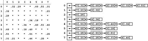
The two standard representations of weighted undirected graphs include weights with each edge representation, as illustrated in the adjacency-matrix (left) and adjacency-lists (right) representation of the graph depicted in Figure 20.1. For simplicity in these figures, we show the weights in the matrix entries and list nodes; in our programs we use pointers to client edges. The adjacency matrix is symmetric and the adjacency lists contain two nodes for each edge, as in unweighted directed graphs. Nonexistent edges are represented null pointers in the matrix (indicated by asterisks in the figure) and are not present at all in the lists. Self-loops are absent in both of the representations illustrated here because MST algorithms are simpler without them; other algorithms that process weighted graphs use them (see Chapter 21).
As with our undirected-graph implementations, we do not explicitly test for parallel edges in either implementation. Depending upon the application, we might alter the adjacency-matrix representation to keep the parallel edge of lowest or highest weight, or to effectively coalesce parallel edges to a single edge with the sum of their weights. In the adjacency-lists representation, we allow parallel edges to remain in the data structure, but we could build more powerful data structures to eliminate them using one of the rules just mentioned for adjacency matrices (see Exercise 17.49).
How should we represent the MST itself? The MST of a graph G is a subgraph of G that is also a tree, so we have numerous options. Chief among them are
• A graph
• A linked list of edges
• A vector of pointers to edges
• A vertex-indexed vector with parent links
Figure 20.4 illustrates these options for the example MST in Figure 20.1. Another alternative is to define and use an ADT for trees.
The same tree might have many different representations in any of the schemes. In what order should the edges be presented in the list-of-edges representation? Which node should be chosen as the root in the parent-link representation (see Exercise 20.21)? Generally speaking, when we run an MST algorithm, the particular MST representation that results is an artifact of the algorithm used and does not reflect any important features of the MST.
Figure 20.4 MST representations
This figure depicts various representations of the MST in Figure 20.1. The most straightforward is a list of its edges, in no particular order (left). The MST is also a sparse graph, and might be represented with adjacency lists (center). The most compact is a parent-link representation: we choose one of the vertices as the root and keep two vertex-indexed vectors, one with the parent of each vertex in the tree, the other with the weight of the edge from each vertex to its parent (right). The orientation of the tree (choice of root vertex) is arbitrary, not a property of the MST. We can convert from any one of these representations to any other in linear time.
From an algorithmic point of view, the choice of MST representation is of little consequence because we can convert easily from each of these representations to any of the others. To convert from the graph representation to a vector of edges, we can use the GRAPHedges function of Program 20.2. To convert from the parent-link representation in a vector st (with weights in another vector wt) to a vector of pointers to edges in mst, we can use the loop
for (k = 1; k < G.V(); k++)
  mst[k] = new EDGE(k, st[k], wt[k]);
This code is for the typical case where the MST is rooted at 0, and it does not put the dummy edge 0-0 onto the MST edge list.
These two conversions are trivial, but how do we convert from the vector-of-edge-pointers representation to the parent-link representation? We have the basic tools to accomplish this task easily as well: We convert to the graph representation using a loop like the one just given (changed to call insert for each edge), then run a a DFS starting at any vertex to compute the parent-link representation of the DFS tree, in linear time.
In short, although the choice of MST representation is a matter of convenience, we package all of our algorithms in a graph-processing class MST that computes a private vector mst of pointers to edges. Depending on the needs of applications, we can implement member functions for this class to return this vector or to give client programs other information about the MST, but we do not specify further details of this interface, other than to include a show member function that calls a similar function for each edge in the MST (see Exercise 20.8).
Exercises
• 20.8 Write a WeightedEdge class that implements the EDGE interface of Program 20.1 and also includes a member function show that prints edges and their weights in the format used in the figures in this chapter.
• 20.9 Implement an io class for weighted graphs that has show, scan, and scanEZ member functions (see Program 17.4).
• 20.10 Build a graph ADT that uses integer weights, but keep track of the minimum and maximum weights in the graph and include an ADT function that always returns weights that are numbers between 0 and 1.
• 20.11 Give an interface like Program 20.1 such that clients and implementations manipulate Edges (not pointers to them).
• 20.12 Develop an implementation of your interface from Exercise 20.11 that uses a minimal matrix-of-weights representation, where the iterator function nxt uses the information implicit in the row and column indices to create an Edge to return to the client.
20.13 Implement the iterator class for use with Program 20.5 (see Program 20.4).
• 20.14 Develop an implementation of your interface from Exercise 20.11 that uses a minimal adjacency-lists representation, where list nodes contain the weight and the destination vertex (but not the source) and the iterator function nxt uses implicit information to create an Edge to return to the client.
• 20.15 Modify the sparse-random-graph generator in Program 17.12 to assign a random weight (between 0 and 1) to each edge.
• 20.16 Modify the dense-random-graph generator in Program 17.13 to assign a random weight (between 0 and 1) to each edge.
20.17 Write a program that generates random weighted graphs by connecting vertices arranged in a V -by- V grid to their neighbors (as in Figure 19.3, but undirected) with random weights (between 0 and 1) assigned to each edge.
20.18 Write a program that generates a random complete graph that has weights chosen from a Gaussian distribution.
• 20.19 Write a program that generates V random points in the plane then builds a weighted graph by connecting each pair of points within a given distance d of one another with an edge whose weight is the distance (see Exercise 17.74). Determine how to set d so that the expected number of edges is E.
• 20.20 Find a large weighted graph online—perhaps a map with distances, telephone connections with costs, or an airline rate schedule.
20.21 Write down an 8-by-8 matrix that contains parent-link representations of all the orientations of the MST of the graph in Figure 20.1. Put the parent-link representation of the tree rooted at i in the ith row of the matrix.
• 20.22 Assume that a MST class constructor produces a vector-of-edge-pointers representation of an MST in mst[1] through mst[V]. Add a member function ST for clients (as in, for example, Program 18.3) such that ST(v) returns v’s parent in the tree (v if it is the root).
• 20.23 Under the assumptions of Exercise 20.22, write a member function that returns the total weight of the MST.
• 20.24 Suppose that a MST class constructor produces a parent-link representation of an MST in a vector st. Give code to be added to the constructor to compute a vector-of-edge-pointers representation in entries 1 through V of a private vector mst.
• 20.25 Define a TREE class. Then, under the assumptions of Exercise 20.22, write a member function that returns a TREE.
20.2 Underlying Principles of MST Algorithms
The MST problem is one of the most heavily studied problems that we encounter in this book. Basic approaches to solving it were invented long before the development of modern data structures and modern techniques for analyzing the performance of algorithms, at a time when finding the MST of a graph that contained, say, thousands of edges was a daunting task. As we shall see, several new MST algorithms differ from old ones essentially in their use and implementation of modern algorithms and data structures for basic tasks, which (coupled with modern computing power) makes it possible for us to compute MSTs with millions or even billions of edges.
One of the defining properties of a tree (see Section 5.4) is that adding an edge to a tree creates a unique cycle. This property is the basis for proving two fundamental properties of MSTs, which we now consider. All the algorithms that we encounter are based on one or both of these two properties.
The first property, which we refer to as the cut property, has to do with identifying edges that must be in an MST of a given graph. The few basic terms from graph theory that we define next make possible a concise statement of this property, which follows.
Definition 20.2 A cut in a graph is a partition of the vertices into two disjoint sets. A crossing edge is one that connects a vertex in one set with a vertex in the other.
We sometimes specify a cut by specifying a set of vertices, leaving implicit the assumption that the cut comprises that set and its complement. Generally, we use cuts where both sets are nonempty—otherwise there are no crossing edges.
Property 20.1 (Cut property) Given any cut in a graph, every minimal crossing edge belongs to some MST of the graph, and every MST contains a minimal crossing edge.
Proof: The proof is by contradiction. Suppose that e is a minimal crossing edge that is not in any MST, and let T be any MST; or suppose that T is an MST that contains no minimal crossing edge, and let e be any minimal crossing edge. In either case, T is an MST that does not contain the minimal crossing edge e. Now consider the graph formed by adding e to T. This graph has a cycle that contains e, and that cycle must contain at least one other crossing edge—say, f, which is equal or higher weight than e (since e is minimal). We can get a spanning tree of equal or lower weight by deleting f and adding e, contradicting either the minimality of T or the assumption that e is not in T.
If a graph’s edge weights are distinct, it has a unique MST; and the cut property says that the shortest crossing edge for every cut must be in the MST. When equal weights are present, we may have multiple minimal crossing edges. At least one of them will be in any given MST and the others may be present or absent.
Figure 20.5 illustrates several examples of this cut property. Note that there is no requirement that the minimal edge be the only MST edge connecting the two sets; indeed, for typical cuts there are several MST edges that connect a vertex in one set with a vertex in the other. If we could be sure that there were only one such edge, we might be able to develop divide-and-conquer algorithms based on judicious selection of the sets; but that is not the case.
We use the cut property as the basis for algorithms to find MSTs, and it also can serve as an optimality condition that characterizes MSTs. Specifically, the cut property implies that every edge in an MST is a minimal crossing edge for the cut defined by the vertices in the two subtrees connected by the edge.
Figure 20.5 Cut property
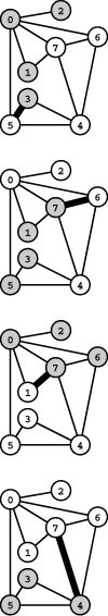
These four examples illustrate Property 20.1. If we color one set of vertices gray and another set white, then the shortest edge connecting a gray vertex with a white one belongs to an MST.
The second property, which we refer to as the cycle property, has to do with identifying edges that do not have to be in a graph’s MST. That is, if we ignore these edges, we can still find an MST.
Property 20.2 (Cycle property) Given a graph G, consider the graph G[prime] defined by adding an edge e to G. Adding e to an MST of G and deleting a maximal edge on the resulting cycle gives an MST of G[prime].
Proof: If e is longer than all the other edges on the cycle, it cannot be on an MST of G [prime], because of Property 20.1: Removing e from any such MST would split the latter into two pieces, and e would not be the shortest edge connecting vertices in each of those two pieces, because some other edge on the cycle must do so. Otherwise, let t be a maximal edge on the cycle created by adding e to the MST of G. Removing t would split the original MST into two pieces, and edges of G connecting those pieces are no shorter than t;so e is a minimal edge in G [prime] connecting vertices in those two pieces. The subgraphs induced by the two subsets of vertices are identical for G and G [prime], so an MST for G [prime] consists of e and the MSTs of those two subsets.
In particular, note that if e is maximal on the cycle, then we have shown that there exists an MST of G [prime] that does not contain e (the MST of G ).
Figure 20.6 illustrates this cycle property. Note that the process of taking any spanning tree, adding an edge that creates a cycle, and then deleting a maximal edge on that cycle gives a spanning tree of weight less than or equal to the original. The new tree weight will be less than the original if and only if the added edge is shorter than some edge on the cycle.
The cycle property also serves as the basis for an optimality condition that characterizes MSTs: It implies that every edge in a graph that is not in a given MST is a maximal edge on the cycle that it forms with MST edges.
The cut property and the cycle property are the basis for the classical algorithms that we consider for the MST problem. We consider edges one at a time, using the cut property to accept them as MST edges or the cycle property to reject them as not needed. The algorithms differ in their approaches to efficiently identifying cuts and cycles.
Figure 20.6 Cycle property
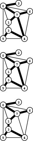
Adding the edge 1-3 to the graph in Figure 20.1 invalidates the MST (top). To find the MST of the new graph, we add the new edge to the MST of the old graph, which creates a cycle (center). Deleting the longest edge on the cycle (4-7) yields the MST of the new graph (bottom). One way to verify that a spanning tree is minimal is to check that each edge not on the MST has the largest weight on the cycle that it forms with tree edges. For example, in the bottom graph, 4-6 has the largest weight on the cycle 4-6-7-1-3-4.
The first approach to finding the MST that we consider in detail is to build the MST one edge at a time: Start with any vertex as a single-vertex MST, then add V − 1 edges to it, always taking next a minimal edge that connects a vertex on the MST to a vertex not yet on the MST. This method is known as Prim’s algorithm; it is the subject of Section 20.3.
Property 20.3 Prim’s algorithm computes an MST of any connected graph.
Proof: As described in detail in Section 20.2, the method is a generalized graph-search method. Implicit in the proof of Property 18.12 is the fact that the edges chosen are a spanning tree. To show that they are an MST, apply the cut property, using vertices on the MST as the first set and vertices not on the MST as the second set.
Another approach to computing the MST is to apply the cycle property repeatedly: We add edges one at a time to a putative MST, deleting a maximal edge on the cycle if one is formed (see Exercises 20.33 and 20.71). This method has received less attention than the others that we consider because of the comparative difficulty of maintaining a data structure that supports efficient implementation of the “delete the longest edge on the cycle” operation.
The second approach to finding the MST that we consider in detail is to process the edges in order of their length (shortest first), adding to the MST each edge that does not form a cycle with edges previously added, stopping after V − 1 edges have been added. This method is known as Kruskal’s algorithm; it is the subject of Section 20.4.
Property 20.4 Kruskal’s algorithm computes an MST of any connected graph.
Proof: We prove by induction that the method maintains a forest of MST subtrees. If the next edge to be considered would create a cycle, it is a maximal edge on the cycle (since all others appeared before it in the sorted order), so ignoring it still leaves an MST, by the cycle property. If the next edge to be considered does not form a cycle, apply the cut property, using the cut defined by the set of vertices connected to one of the edge’s vertex by MST edges (and its complement). Since the edge does not create a cycle, it is the only crossing edge, and since we consider the edges in sorted order, it is a minimal edge and therefore in an MST. The basis for the induction is the V individual vertices; once we have chosen V − 1 edges, we have one tree (the MST). No unexamined edge is shorter than an MST edge, and all would create a cycle, so ignoring all of the rest of the edges leaves an MST, by the cycle property.
The third approach to building an MST that we consider in detail is known as Boruvka’s algorithm; it is the subject of Section 20.4. The first step is to add to the MST the edges that connect each vertex to its closest neighbor. If edge weights are distinct, this step creates a forest of MST subtrees (we prove this fact and consider a refinement that does so even when equal-weight edges are present in a moment). Then, we add to the MST the edges that connect each tree to a closest neighbor (a minimal edge connecting a vertex in one tree with a vertex in any other), and iterate the process until we are left with just one tree.
Property 20.5 Boruvka’s algorithm computes the MST of any connected graph.
First, suppose that the edge weights are distinct. In this case, each vertex has a unique closest neighbor, the MST is unique, and we know that each edge added is an MST edge by applying the cut property (it is the shortest edge crossing the cut from a vertex to all the other vertices). Since every edge chosen is from the unique MST, there can be no cycles, each edge added merges two trees from the forest into a bigger tree, and the process continues until a single tree, the MST, remains.
If edge weights are not distinct, there may be more than one closest neighbor, and a cycle could form when we add the edges to closest neighbors (see Figure 20.7). Put another way, we might include two edges from the set of minimal crossing edges for some vertex, when only one belongs on the MST. To avoid this problem, we need an appropriate tie-breaking rule. One choice is to choose, among the minimal neighbors, the one with the lowest vertex number. Then any cycle would present a contradiction: If v is the highest-numbered vertex in the cycle, then neither neighbor of v would have led to its choice as the closest, and v would have led to the choice of only one of its lower-numbered neighbors, not both.
Figure 20.7 Cycles in Boruvka’s algorithm
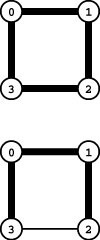
In the graph of four vertices and four edges shown here, the edges are all the same length. When we connect each vertex to a nearest neighbor, we have to make a choice between minimal edges. In the example at the top, we choose 1 from 0, 2 from 1, 3 from 2, and 0 from 3, which leads to a cycle in the putative MST. Each of the edges are in some MST, but not all are in every MST. To avoid this problem, we adopt a tie-breaking rule, as shown in the bottom: Choose the minimal edge to the vertex with the lowest index. Thus, we choose 1 from 0, 0 from 1, 1 from 2, and 0 from 3, which yields an MST. The cycle is broken because highest-numbered vertex 3 is not chosen from either of its neighbors 2 or 1, and it can choose only one of them (0).
These algorithms are all special cases of a general paradigm that is still being used by researchers seeking new MST algorithms. Specifically, we can apply in arbitrary order the cut property to accept an edge as an MST edge or the cycle property to reject an edge, continuing until neither can increase the number of accepted or rejected edges. At that point, any division of the graph’s vertices into two sets has an MST edge connecting them (so applying the cut property cannot increase the number of MST edges), and all graph cycles have at least one non-MST edge (so applying the cycle property cannot increase the number of non-MST edges). Together, these properties imply that a complete MST has been computed.
More specifically, the three algorithms that we consider in detail can be unified with a generalized algorithm where we begin with a forest of single-vertex MST subtrees (each with no edges) and perform the step of adding to the MST a minimal edge connecting any two subtrees in the forest, continuing until V − 1 edges have been added and a single MST remains. By the cut property, no edge that causes a cycle need be considered for the MST, since some other edge was previously a minimal edge crossing a cut between MST subtrees containing each of its vertices. With Prim’s algorithm, we grow a single tree an edge at a time; with Kruskal’s and Boruvka’s algorithms, we coalesce trees in a forest.
As described in this section and in the classical literature, the algorithms involve certain high-level abstract operations, such as the following:
• Find a minimal edge connecting two subtrees.
• Determine whether adding an edge would create a cycle.
• Delete the longest edge on a cycle.
Our challenge is to develop algorithms and data structures that implement these operations efficiently. Fortunately, this challenge presents us with an opportunity to put to good use basic algorithms and data structures that we developed earlier in this book.
MST algorithms have a long and colorful history that is still evolving; we discuss that history as we consider them in detail. Our evolving understanding of different methods of implementing the basic abstract operations has created some confusion surrounding the origins of the algorithms over the years. Indeed, the methods were first described in the 1920s, pre-dating the development of computers as we know them, as well as pre-dating our basic knowledge about sorting and other algorithms. As we now know, the choices of underlying algorithm and data structure can have substantial influences on performance, even when we are implementing the most basic schemes. In recent years, research on the MST problem has concentrated on such implementation issues, still using the classical schemes. For consistency and clarity, we refer to the basic approaches by the names listed here, although abstract versions of the algorithms were considered earlier, and modern implementations use algorithms and data structures invented long after these methods were first contemplated.
As yet unsolved in the design and analysis of algorithms is the quest for a linear-time MST algorithm. As we shall see, many of our implementations are linear-time in a broad variety of practical situations, but they are subject to a nonlinear worst case. The development of an algorithm that is guaranteed to be linear-time for sparse graphs is still a research goal.
Beyond our normal quest in search of the best algorithm for this fundamental problem, the study of MST algorithms underscores the importance of understanding the basic performance characteristics of fundamental algorithms. As programmers continue to use algorithms and data structures at increasingly higher levels of abstraction, situations of this sort become increasingly common. Our ADT implementations have varying performance characteristics—as we use higher-level ADTs as components when solving more yet higher-level problems, the possibilities multiply. Indeed, we often use algorithms that are based on using MSTs and similar abstractions (enabled by the efficient implementations that we consider in this chapter) to help us solve other problems at a yet higher level of abstraction.
Exercises
• 20.26 Label the following points in the plane 0 through 5, respectively:
(1, 3) (2, 1) (6, 5) (3, 4) (3, 7) (5, 3).
Taking edge lengths to be weights, give an MST of the graph defined by the edges
1-0 3-5 5-2 3-4 5-1 0-3 0-4 4-2 2-3.
20.27 Suppose that a graph has distinct edge weights. Does its shortest edge have to belong to the MST? Prove that it does or give a counterexample.
20.28 Answer Exercise 20.27 for the graph’s longest edge.
20.29 Give a counterexample that shows why the following strategy does not necessarily find the MST:
“Start with any vertex as a single-vertex MST, then add V − 1 edges to it, always taking next a minimal edge incident upon the vertex most recently added to the MST.”
20.30 Suppose that a graph has distinct edge weights. Does a minimal edge on every cycle have to belong to the MST? Prove that it does or give a counterexample.
20.31 Given an MST for a graph G, suppose that an edge in G is deleted. Describe how to find an MST of the new graph in time proportional to the number of edges in G.
20.32 Show the MST that results when you repeatedly apply the cycle property to the graph in Figure 20.1, taking the edges in the order given.
20.33 Prove that repeated application of the cycle property gives an MST.
20.34 Describe how each of the algorithms described in this section can be adapted (if necessary) to the problem of finding a minimal spanning forest of a weighted graph (the union of the MSTs of its connected components).
20.3 Prim’s Algorithm and Priority-First Search
Prim’s algorithm is perhaps the simplest MST algorithm to implement, and it is the method of choice for dense graphs. We maintain a cut of the graph that is comprised of tree vertices (those chosen for the MST) and nontree vertices (those not yet chosen for the MST). We start by putting any vertex on the MST, then put a minimal crossing edge on the MST (which changes its nontree vertex to a tree vertex) and repeat the same operation V − 1 times, to put all vertices on the tree.
A brute-force implementation of Prim’s algorithm follows directly from this description. To find the edge to add next to the MST, we could examine all the edges that go from a tree vertex to a nontree vertex, then pick the shortest of the edges found to put on the MST. We do not consider this implementation here because it is overly expensive (see Exercises 20.35 through 20.37). Adding a simple data structure to eliminate excessive recomputation makes the algorithm both simpler and faster.
Adding a vertex to the MST is an incremental change: To implement Prim’s algorithm, we focus on the nature of that incremental change. The key is to note that our interest is in the shortest distance from each nontree vertex to the tree. When we add a vertex v to the tree, the only possible change for each nontree vertex w is that adding
Figure 20.8 Prim’s MST algorithm
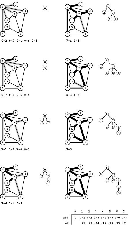
The first step in computing the MST with Prim’s algorithm is to add 0 to the tree. Then we find all the edges that connect 0 to other vertices (which are not yet on the tree) and keep track of the shortest (top left). The edges that connect tree vertices with nontree vertices (the fringe) are shadowed in gray and listed below each graph drawing. For simplicity in this figure, we list the fringe edges in order of their length so that the shortest is the first in the list. Different implementations of Prim’s algorithm use different data structures to maintain this list and to find the minimum. The second step is to move the shortest edge 0-2 (along with the vertex that it takes us to) from the fringe to the tree (second from top, left). Third, we move 0-7 from the fringe to the tree, replace 0-1 by 7-1 and 0-6 by 7-6 on the fringe (because adding 7 to the tree brings 1 and 6 closer to the tree), and add 7-4 to the fringe (because adding 7 to the tree makes 7-4 an edge that connects a tree vertex with a nontree vertex) (third from top, left). Next, we move edge 7-1 to the tree (bottom, left). To complete the computation, we take 7-6, 7-4, 4-3, and 3-5 off the queue, updating the fringe after each insertion to reflect any shorter or new paths discovered (right, top to bottom).
An oriented drawing of the growing MST is shown at the right of each graph drawing. The orientation is an artifact of the algorithm: We generally view the MST itself as a set of edges, unordered and unoriented.
v brings w closer than before to the tree. In short, we do not need to check the distance from w to all tree vertices—we just need to keep track of the minimum and check whether the addition of v to the tree necessitates that we update that minimum.
To implement this idea, we need data structures that can give us the following information:
• The tree edges
• The shortest edge connecting each nontree vertex to the tree
• The length of that edge
The simplest implementation for each of these data structures is a vertex-indexed vector (we can use such a vector for the tree edges by indexing on vertices as they are added to the tree). Program 20.6 is an implementation of Prim’s algorithm for dense graphs. It uses the vectors mst, fr, and wt (respectively) for these three data structures.
After adding a new edge (and vertex) to the tree, we have two tasks to accomplish:
• Check to see whether adding the new edge brought any nontree vertex closer to the tree.
• Find the next edge to add to the tree.
The implementation in Program 20.6 accomplishes both of these tasks with a single scan through the nontree vertices, updating wt[w] and fr[w] if v-w brings w closer to the tree, then updating the current minimum if wt[w] (the length of fr[w]) indicates that w is closer to the tree than any other nontree vertex with a lower index).
Property 20.6 Using Prim’s algorithm, we can find the MST of a dense graph in linear time.
Proof: It is immediately evident from inspection of the program that the running time is proportional to V2 and therefore is linear for dense graphs.
Figure 20.8 shows an example MST construction with Prim’s algorithm; Figure 20.9 shows the evolving MST for a larger example.
Program 20.6 is based on the observation that we can interleave the find the minimum and update operations in a single loop where we examine all the nontree edges. In a dense graph, the number of edges that we may have to examine to update the distance from the nontree vertices to the tree is proportional to V, so looking at all the nontree edges to find the one that is closest to the tree does not represent
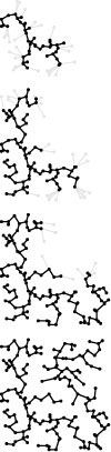
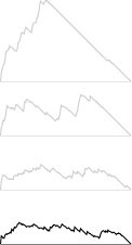
Figure 20.9 Prim’s MST algorithm

This sequence shows how the MST grows as Prim’s algorithm discovers 1/4, 1/2, 3/4, and all of the edges in the MST (top to bottom). An oriented representation of the full MST is shown at the right.
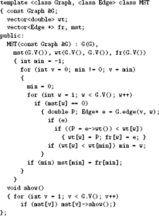
Program 20.6 Prim’s MST algorithm
This implementation of Prim’s algorithm is the method of choice for dense graphs and can be used for any graph representation that supports the edge existence test. The outer loop grows the MST by choosing a minimal edge crossing the cut between the vertices on the MST and vertices not on the MST. The w loop finds the minimal edge while at the same time (if w is not on the MST) maintaining the invariant that the edge fr[w] is the shortest edge (of weight wt[w]) from w to the MST.
The result of the computation is a vector of edge pointers. The first (mst[0]) is unused; the rest (mst[1] through mst[G.V()]) comprise the MST of the connected component of the graph that contains 0.
excessive extra cost. But in a sparse graph, we can expect to use substantially fewer than V steps to perform each of these operations. The crux of the strategy that we will use to do so is to focus on the set of potential edges to be added next to the MST—a set that we call the fringe. The number of fringe edges is typically substantially smaller than the number of nontree edges, and we can recast our description of the algorithm as follows. Starting with a self loop to a start vertex on the fringe and an empty tree, we perform the following operation until the fringe is empty:
Move a minimal edge from the fringe to the tree. Visit the vertex that it leads to, and put onto the fringe any edges that lead from that vertex to an nontree vertex, replacing the longer edge when two edges on the fringe point to the same vertex.
From this formulation, it is clear that Prim’s algorithm is nothing more than a generalized graph search (see Section 18.8), where the fringe is a priority queue based on a remove the minimum operation (see Chapter 9). We refer to generalized graph searching with priority queues as priority-first search (PFS). With edge weights for priorities, PFS implements Prim’s algorithm.
This formulation encompasses a key observation that we made already in connection with implementing BFS in Section 18.7. An even simpler general approach is to simply keep on the fringe all of the edges that are incident upon tree vertices, letting the priority-queue mechanism find the shortest one and ignore longer ones (see Exercise 20.41). As we saw with BFS, this approach is unattractive because the fringe data structure becomes unnecessarily cluttered with edges that will never get to the MST. The size of the fringe could grow to be proportional to E (with whatever attendant costs having a fringe this size might involve), while the PFS approach just outlined ensures that the fringe will never have more than V entries.
As with any implementation of a general algorithm, we have a number of available approaches for interfacing with priority-queue ADTs. One approach is to use a priority queue of edges, as in our generalized graph-search implementation of Program 18.10. Program 20.7 is an implementation that is essentially equivalent to Program 18.10 but uses a vertex-based approach so that it can use an indexed priority-queue, as described in Section 9.6. (We consider a complete implemen tation of the specific priority-queue interface used by Program 20.7 is at the end of this chapter, in Program 20.10.) We identify the fringe vertices, the subset of nontree vertices that are connected by fringe edges to tree vertices, and keep the same vertex-indexed vectors mst, fr, and wt as in Program 20.6. The priority queue contains the index of each fringe vertex, and that entry gives access to the shortest edge connecting the fringe vertex with the tree and the length of that edge, through the second and third vectors.
The first call to pfs in the constructor in Program 20.7 finds the MST in the connected component that contains vertex 0, and subsequent calls find MSTs in other components, so this class actually finds minimal spanning forests in graphs that are not connected (see Exercise 20.34).
Property 20.7 Using a PFS implementation of Prim’s algorithm that uses a heap for the priority-queue implementation, we can compute an MST in time proportional to E lg V.
Proof: The algorithm directly implements the generic idea of Prim’s algorithm (add next to the MST a minimal edge that connects a vertex on the MST with a vertex not on the MST). Each priority-queue operation requires less than lg V steps. Each vertex is chosen with a remove the minimum operation; and, in the worst case, each edge might require a change priority operation.
Priority-first search is a proper generalization of breadth-first and depth-first search because those methods also can be derived through appropriate priority settings. For example, we can (somewhat artificially) use a variable cnt to assign a unique priority cnt++ to each vertex when we put that vertex on the priority queue. If we define P to be cnt, we get preorder numbering and DFS because newly encountered nodes have the highest priority. If we define P to be V-cnt, we get BFS because old nodes have the highest priority. These priority assignments make the priority queue operate like a stack and a queue, respectively. This equivalence is purely of academic interest since the priority-queue operations are unnecessary for DFS and BFS. Also, as discussed in Section 18.8, a formal proof of equivalence would require a precise attention to replacement rules to obtain the same sequence of vertices as result from the classical algorithms.
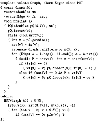
Program 20.7 Priority-first search
The function pfs is a generalized graph search that uses a priority queue for the fringe (see Section 18.8). The priority P is defined such that this class implements Prim’s MST algorithm; other priority definitions give other algorithms. The main loop moves the highest-priority (lowest-weight) edge from the fringe to the tree, then checks every edge adjacent to the new tree vertex to see whether it implies changes in the fringe. Edges to vertices not on the fringe or the tree are added to the fringe; shorter edges to fringe vertices replace corresponding fringe edges.
The PQi class is an indirect priority-queue interface (see Section 9.6) modified to pass a reference to the priority array to the constructor, to substitute getmin for delmax, and to substitute lower for change. Program 20.10 is an implementation of this interface.
As we shall see, PFS encompasses not just DFS, BFS, and Prim’s MST algorithm but also several other classical algorithms. The various algorithms differ only in their priority functions. Thus, the running times of all these algorithms depend on the performance of the priority-queue ADT. Indeed, we are led to a general result that encompasses not just the two implementations of Prim’s algorithms that we have examined in this section but also a broad class of fundamental graph-processing algorithms.
Property 20.8 For all graphs and all priority functions, we can compute a spanning tree with PFS in linear time plus time proportional to the time required for V insert, V delete the minimum, and E decrease key operations in a priority queue of size at most V.
Proof: The proof of Property 20.7 establishes this more general result. We have to examine all the edges in the graph; hence the “linear time” clause. The algorithm never increases the priority (it changes the priority to only a lower value); by more precisely specifying what we need from the priority-queue ADT ( decrease key, not necessarily change priority ), we strengthen this statement about performance.
In particular, use of an unordered-array priority-queue implementation gives an optimal solution for dense graphs that has the same worst-case performance as the classical implementation of Prim’s algorithm (Program 20.6). That is, Properties 20.6 and 20.7 are special cases of Property 20.8; throughout this book we shall see numerous other algorithms that essentially differ in only their choice of priority function and their priority-queue implementation.
Property 20.7 is an important general result: The time bound stated is a worst-case upper bound that guarantees performance within a factor of lg V of optimal (linear time) for a large class of graph-processing problems. Still, it is somewhat pessimistic for many of the graphs that we encounter in practice, for two reasons. First, the lg V bound for priority-queue operation holds only when the number of vertices on the fringe is proportional to V, and even then it is just an upper bound. For a real graph in a practical application, the fringe might be small (see Figures 20.10 and 20.11), and some priority-queue operations might take many fewer than lg V steps. Although noticeable, this effect is likely to account for only a small constant factor in the running time; for example, a proof that the fringe never has more than pV vertices on it would improve the bound by only a factor of 2. More important, we generally perform many fewer than E decrease key operations since we do that operation only when we find an edge to a fringe node that is shorter than the current best-known edge to a fringe node. This event is relatively rare: Most edges have no effect on the priority queue (see Exercise 20.40). It is reasonable to regard PFS as an essentially linear-time algorithm unless V lg V is significantly greater than E.
Figure 20.10 PFS implementation of Prim’s MST algorithm
With PFS, Prim’s algorithm processes just the vertices and edges closest to the MST (in gray).
Figure 20.11 Fringe size for PFS implementation of Prim’s algorithm
The plot at the bottom shows the size of the fringe as the PFS proceeds for the example in Figure 20.10. For comparison, the corresponding plots for DFS, randomized search, and BFS from Figure 18.28 are shown above in gray.
The priority-queue ADT and generalized graph-searching abstractions make it easy for us to understand the relationships among various algorithms. Since these abstractions (and software mechanisms to support their use) were developed many years after the basic methods, relating the algorithms to classical descriptions of them becomes an exercise for historians. However, knowing basic facts about the history is useful when we encounter descriptions of MST algorithms in the research literature or in other texts, and understanding how these few simple abstractions tie together the work of numerous researchers over a time span of decades is persuasive evidence of their value and power. Thus, we consider briefly the origins of these algorithms here.
An MST implementation for dense graphs essentially equivalent to Program 20.6 was first presented by Prim in 1961, and, independently, by Dijkstra soon thereafter. It is usually referred to as Prim’s algorithm, although Dijkstra’s presentation was more general, so some scholars refer to the MST algorithm as a special case of Dijkstra’s algorithm. But the basic idea was also presented by Jarnik in 1939, so some authors refer to the method as Jarnik’s algorithm, thus characterizing Prim’s (or Dijkstra’s) role as finding an efficient implementation of the algorithm for dense graphs. As the priority-queue ADT came into use in the early 1970s, its application to finding MSTs of sparse graphs was straightforward; the fact that MSTs of sparse graphs could be computed in time proportional to E lg V became widely known without attribution to any particular researcher. Since that time, as we discuss in Section 20.6, many researchers have concentrated on finding efficient priority-queue implementations as the key to finding efficient MST algorithms for sparse graphs.
Exercises
• 20.35 Analyze the performance of the brute-force implementation of Prim’s algorithm mentioned at the beginning of this section for a complete weighted graph with V vertices. Hint: The following combinatorial sum might be useful:Σ1k<V k (V−k) = (V+1) V (V−1) /6.
• 20.36 Answer Exercise 20.35 for graphs in which all vertices have the same fixed degree t.
• 20.37 Answer Exercise 20.35 for general sparse graphs that have V vertices and E edges. Since the running time depends on the weights of the edges and on the degrees of the vertices, do a worst-case analysis. Exhibit a family of graphs for which your worst-case bound is confirmed.
20.38 Show, in the style of Figure 20.8, the result of computing the MST of the network defined in Exercise 20.26 with Prim’s algorithm.
• 20.39 Describe a family of graphs with V vertices and E edges for which the worst-case running time of the PFS implementation of Prim’s algorithm is confirmed.
•• 20.40 Develop a reasonable generator for random graphs with V vertices and E edges such that the running time of the PFS implementation of Prim’s algorithm (Program 20.7) is nonlinear.
• 20.41 Modify Program 20.7 so that it works like Program 18.8, in that it keeps on the fringe all edges incident upon tree vertices. Run empirical studies to compare your implementation with Program 20.7, for various weighted graphs (see Exercises 20.9–14).
20.42 Derive a priority queue implementation for use by Program 20.7 from the interface defined in Program 9.12 (so any implementation of that interface could be used).
20.43 Use the STL priority_queue to implement the priority-queue interface that is used by Program 20.7.
20.44 Suppose that you use a priority-queue implementation that maintains a sorted list. What would be the worst-case running time for graphs with V vertices and E edges, to within a constant factor? When would this method be appropriate, if ever? Defend your answer.
• 20.45 An MST edge whose deletion from the graph would cause the MST weight to increase is called a critical edge. Show how to find all critical edges in a graph in time proportional to E lg V.
20.46 Run empirical studies to compare the performance of Program 20.6 to that of Program 20.7, using an unordered array implementation for the priority queue, for various weighted graphs (see Exercises 20.9–14).
• 20.47 Run empirical studies to determine the effect of using an index-heap– tournament (see Exercise 9.53) priority-queue implementation instead of Program 9.12 in Program 20.7, for various weighted graphs (see Exercises 20.9– 14).
20.48 Run empirical studies to analyze tree weights (see Exercise 20.23) as a function of V, for various weighted graphs (see Exercises 20.9–14).
20.49 Run empirical studies to analyze maximum fringe size as a function of V, for various weighted graphs (see Exercises 20.9–14).
20.50 Run empirical studies to analyze tree height as a function of V, for various weighted graphs (see Exercises 20.9–14).
20.51 Run empirical studies to study the dependence of the results of Exercises 20.49 and 20.50 on the start vertex. Would it be worthwhile to use a random starting point?
• 20.52 Write a client program that does dynamic graphical animations of Prim’s algorithm. Your program should produce images like Figure 20.10 (see Exercises 17.56 through 17.60). Test your program on random Euclidean neighbor graphs and on grid graphs (see Exercises 20.17 and 20.19), using as many points as you can process in a reasonable amount of time.
20.4 Kruskal’s Algorithm
Prim’s algorithm builds the MST one edge at a time, finding a new edge to attach to a single growing tree at each step. Kruskal’s algorithm also builds the MST one edge at a time; but, by contrast, it finds an edge that connects two trees in a spreading forest of growing MST subtrees. We start with a degenerate forest of V single-vertex trees and perform the operation of combining two trees (using the shortest edge possible) until there is just one tree left: the MST.
Figure 20.12 shows a step-by-step example of the operation of Kruskal’s algorithm; Figure 20.13 illustrates the algorithm’s dynamic characteristics on a larger example. The disconnected forest of MST subtrees evolves gradually into a tree. Edges are added to the MST in order of their length, so the forests comprise vertices that are connected to one another by relatively short edges. At any point during the execution of the algorithm, each vertex is closer to some vertex in its subtree than to any vertex not in its subtree.
Kruskal’s algorithm is simple to implement, given the basic algorithmic tools that we have considered in this book. Indeed, we can use any sort from Part 3 to sort the edges by weight and any of the connectivity algorithms from Chapter 1 to eliminate those that cause cycles! Program 20.8 is an implementation along these lines of an MST function for a graph ADT that is functionally equivalent to the other MST implementations that we consider in this chapter. The implementation does not depend on the graph representation: It calls a GRAPH client to return a vector that contains the graph’s edges, then computes the MST from that vector.
Figure 20.12 Kruskal’s MST algorithm
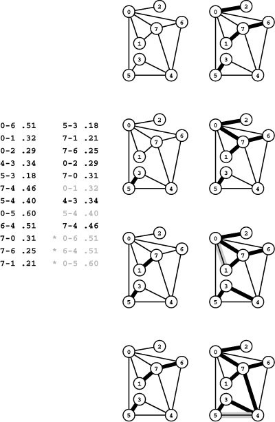
Given a list of a graph’s edges in arbitrary order (left edge list), the first step in Kruskal’s algorithm is to sort them by weight (right edge list). Then we go through the edges on the list in order of their weight, adding edges that do not create cycles to the MST. We add 5-3 (the shortest edge), then 7-1, then 7-6 (left), then 0-2 (right, top) and 0-7 (right, second from top). The edge with the next largest weight, 0-1, creates a cycle and is not included. Edges that we do not add to the MST are shown in gray on the sorted list. Then we add 4-3 (right, third from top). Next, we reject 5-4 because it causes a cycle, then we add 7-4 (right, bottom). Once the MST is complete, any edges with larger weights would cause cycles and be rejected (we stop when we have added V-1 edges to the MST). These edges are marked with asterisks on the sorted list.
Note that there are two ways in which Kruskal’s algorithm can terminate. If we find V − 1 edges, then we have a spanning tree and can stop. If we examine all the edges without finding V −1 tree edges, then we have determined that the graph is not connected, precisely as we did in Chapter 1.
Analyzing the running time of Kruskal’s algorithm is a simple matter because we know the running time of its constituent ADT operations.
Property 20.9 Kruskal’s algorithm computes the MST of a graph in time proportional to E lg E.
Proof: This property is a consequence of the more general observation that the running time of Program 20.8 is proportional to the cost of sorting E numbers plus the cost of E find and V − 1 union operations. If we use standard ADT implementations such as mergesort and weighted union-find with halving, the cost of sorting dominates.
We consider the comparative performance of Kruskal’s and Prim’s algorithm in Section 20.6. For the moment, note that a running time proportional to E lg E is not necessarily worse than E lg V, because E is at most V2, so lg E is at most 2lg V. Performance differences for specific graphs are due to what the properties of the implementations are and to whether the actual running time approaches these worst-case bounds.
In practice, we might use quicksort or a fast system sort (which is likely to be based on quicksort). Although this approach may give the usual unappealing (in theory) quadratic worst case for the sort, it is likely to lead to the fastest run time. Indeed, on the other hand, we could use a radix sort to do the sort in linear time (under certain conditions on the weights) so that the cost of the E find operations dominates and then adjust Property 20.9 to say that the running time of Kruskal’s algorithm is within a constant factor of E lg*E under those conditions on the weights (see Chapter 2). Recall that the function lg*E is the number of iterations of the binary logarithm function before the result is less than 1, which is less than 5 if E is less than 265536. In other words, these adjustments make Kruskal’s algorithm effectively linear in most practical circumstances.
Figure 20.13 Kruskal’s MST algorithm

This sequence shows 1 / 4, 1 / 2, 3 / 4, and the full MST as it evolves.
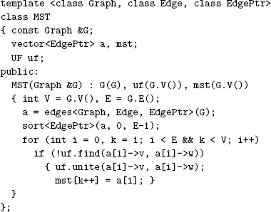
Program 20.8 Kruskal’s MST algorithm
This implementation uses our sorting ADT from Chapter 6 and our union-find ADT from Chapter 4 to find the MST by considering the edges in order of their weights, discarding edges that create cycles until finding V − 1 edges that comprise a spanning tree.
Not shown are a wrapper class EdgePtr that wraps pointers to Edges so sort can compare them using an overloaded <, as described in Section 6.8, and a version of Program 20.2 with a third template argument.
Typically, the cost of finding the MST with Kruskal’s algorithm is even lower than the cost of processing all edges because the MST is complete well before a substantial fraction of the (long) graph edges is ever considered. We can take this fact into account to reduce the running time significantly in many practical situations by keeping edges that are longer than the longest MST edge entirely out of the sort. One easy way to accomplish this objective is to use a priority queue, with an implementation that does the construct operation in linear time and the remove the minimum operation in logarithmic time.
For example, we can achieve these performance characteristics with a standard heap implementation, using bottom-up construction (see Section 9.4). Specifically, we make the following changes to Program 20.8: First, we change the call on sort to a call on pq.construct() to build a heap in time proportional to E. Second, we change the inner loop to take the shortest edge off the priority queue with e = pq.delmin() and to change all references to a[i] to refer to e.
Property 20.10 A priority-queue–based version of Kruskal’s algorithm computes the MST of a graph in time proportional to E + X lg V, where X is the number of graph edges not longer than the longest edge in the MST.
Proof: See the preceding discussion, which shows the cost to be the cost of building a priority queue of size E plus the cost of running the X delete the minimum, X find, and V −1 union operations. Note that the priority-queue–construction costs − dominate (and the algorithm is linear time) unless X is greater than E/ lg V.
We can also apply the same idea to reap similar benefits in a quicksort-based implementation. Consider what happens when we use a straight recursive quicksort, where we partition at i, then recursively sort the subfile to the left of i and the subfile to the right of i. We note that, by construction of the algorithm, the first i elements are in sorted order after completion of the first recursive call (see Program 9.2). This obvious fact leads immediately to a fast implementation of Kruskal’s algorithm: If we put the check for whether the edge a[i] causes a cycle between the recursive calls, then we have an algorithm that, by construction, has checked the first i edges, in sorted order, after completion of the first recursive call! If we include a test to return when we have found V-1 MST edges, then we have an algorithm that sorts only as many edges as we need to compute the MST, with a few extra partitioning stages involving larger elements (see Exercise 20.57). Like straight sorting implementations, this algorithm could run in quadratic time in the worst case, but we can provide a probabilistic guarantee that the worst-case running time will not come close to this limit. Also, like straight sorting implementations, this program is likely to be faster than a heap-based implementation because of its shorter inner loop.
If the graph is not connected, the partial-sort versions of Kruskal’s algorithm offer no advantage because all the edges have to be considered. Even for a connected graph, the longest edge in the graph might be in the MST, so any implementation of Kruskal’s method would still have to examine all the edges. For example, the graph might consist of tight clusters of vertices all connected together by short edges, with one outlier connected to one of the vertices by a long edge. Despite such anomalies, the partial-sort approach is probably worthwhile because it offers significant gain when it applies and incurs little if any extra cost.
Historical perspective is relevant and instructive here as well. Kruskal presented this algorithm in 1956, but, again, the relevant ADT implementations were not carefully studied for many years, so the performance characteristics of implementations such as the priority-queue version of Program 20.8 were not well understood until the 1970s. Other interesting historical notes are that Kruskal’s paper mentioned a version of Prim’s algorithm (see Exercise 20.59) and that Boruvka mentioned both approaches. Efficient implementations of Kruskal’s method for sparse graphs preceded implementations of Prim’s method for sparse graphs because union-find (and sort) ADTs came into use before priority-queue ADTs. Generally, as was true of implementations of Prim’s algorithm, advances in the state of the art for Kruskal’s algorithm are attributed primarily to advances in ADT performance. On the other hand, the applicability of the union-find abstraction to Kruskal’s algorithm and the applicability of the priority-queue abstraction to Prim’s algorithm have been prime motivations for many researchers to seek better implementations of those ADTs.
Exercises
• 20.53 Show, in the style of Figure 20.12, the result of computing the MST of the network defined in Exercise 20.26 with Kruskal’s algorithm.
• 20.54 Run empirical studies to analyze the length of the longest edge in the MST and the number of graph edges that are not longer than that one, for various weighted graphs (see Exercises 20.9–14).
• 20.55 Develop an implementation of the union-find ADT that implements find in constant time and union in time proportional to lg V.
20.56 Run empirical tests to compare your ADT implementation from Exercise 20.55 to weighted union-find with halving (Program 1.4) when Kruskal’s algorithm is the client, for various weighted graphs (see Exercises 20.9–14). Separate out the cost of sorting the edges so that you can study the effects of the change both on the total cost and on the part of the cost associated with the union-find ADT.
20.57 Develop an implementation based on the idea described in the text where we integrate Kruskal’s algorithm with quicksort so as to check MST membership of each edge as soon as we know that all smaller edges have been checked.
• 20.58 Adapt Kruskal’s algorithm to implement two ADT functions that fill a client-supplied vertex-indexed vector classifying vertices into k clusters with the property that no edge of length greater than d connects two vertices in different clusters. For the first function, take k as an argument and return d; for the second, take d as an argument and return k. Test your program on random Euclidean neighbor graphs and on grid graphs (see Exercises 20.17 and 20.19) of various sizes for various values of k and d.
20.59 Develop an implementation of Prim’s algorithm that is based on pre-sorting the edges.
• 20.60 Write a client program that does dynamic graphical animations of Kruskal’s algorithm (see Exercise 20.52). Test your program on random Euclidean neighbor graphs and on grid graphs (see Exercises 20.17 and 20.19), using as many points as you can process in a reasonable amount of time.
Figure 20.14 Boruvka’s MST algorithm
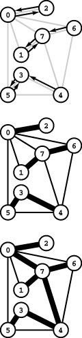
The diagram at the top shows a directed edge from each vertex to its closest neighbor. These edges show that 0-2, 1-7, and 3-5 are each the shortest edge incident on both their vertices, 6-7 is 6’s shortest edge, and 4-3 is 4’s shortest edge. These edges all belong to the MST and comprise a forest of MST subtrees (center), as computed by the first phase of Boruvka’s algorithm. In the second phase, the algorithm completes the MST computation (bottom) by adding the edge 0-7, which is the shortest edge incident on any of the vertices in the subtrees it connects, and the edge 4-7, which is the shortest edge incident on any of the vertices in the bottom subtree.
20.5 Boruvka’s Algorithm
The next MST algorithm that we consider is also the oldest. Like Kruskal’s algorithm, we build the MST by adding edges to a spreading forest of MST subtrees; but we do so in stages, adding several MST edges at each stage. At each stage, we find the shortest edge that connects each MST subtree with a different one, then add all such edges to the MST.
Again, our union-find ADT from Chapter 1 leads to an efficient implementation. For this problem, it is convenient to extend the interface to make the find operation available to clients. We use this function to associate an index with each subtree so that we can tell quickly to which subtree a given vertex belongs. With this capability, we can implement efficiently each of the necessary operations for Boruvka’s algorithm.
First, we maintain a vertex-indexed vector that identifies, for each MST subtree, the nearest neighbor. Then, we perform the following operations on each edge in the graph:
• If it connects two vertices in the same tree, discard it.
• Otherwise, check the nearest-neighbor distances between the two trees the edge connects and update them if appropriate.
After this scan of all the graph edges, the nearest-neighbor vector has the information that we need to connect the subtrees. For each vertex index, we perform a union operation to connect it with its nearest neighbor. In the next stage, we discard all the longer edges that connect other pairs of vertices in the now-connected MST subtrees. Figures 20.14 and 20.15 illustrate this process on our sample algorithm
Program 20.9 is a direct implementation of Boruvka’s algorithm. There are three major factors that make this implementation efficient:
• The cost of each find operation is essentially constant.
• Each stage decreases the number of MST subtrees in the forest by at least a factor of 2.
• A substantial number of edges is discarded during each stage. It is difficult to quantify precisely all these factors, but the following bound is easy to establish.
Property 20.11 The running time of Boruvka’s algorithm for computing the MST of a graph is O ( E lg V lg*E) .
Proof: Since the number of trees in the forest is halved at each stage, the number of stages is no larger than lg V. The time for each stage is at most proportional to the cost of E find operations, which is less than E lg*E, or linear for practical purposes.
The running time given in Property 20.11 is a conservative upper bound since it does not take into account the substantial reduction in the number of edges during each stage. The find operations take constant time in the early passes, and there are very few edges in the later passes. Indeed, for many graphs, the number of edges decreases exponentially with the number of vertices, and the total running time is proportional to E. For example, as illustrated in Figure 20.16, the algorithm finds the MST of our larger sample graph in just four stages.
It is possible to remove the lg*E factor to lower the theoretical bound on the running time of Boruvka’s algorithm to be proportional to E lg V, by representing MST subtrees with doubly-linked lists instead of using the union and find operations. However, this improvement is sufficiently more complicated to implement and the potential performance improvement sufficiently marginal that it is not likely to be worth considering for use in practice (see Exercises 20.66 and 20.67).
Figure 20.15 Union-find array in Boruvka’s algorithm
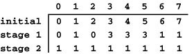
This figure depicts the contents of the union-find array corresponding to the example depicted in Figure 20.14. Initially, each entry contains its own index, indicating a forest of singleton vertices. After the first stage, we have three components, represented by the indices 0, 1, and 3 (the union-find trees are all flat for this tiny example). After the second stage, we have just one component, represented by 1.
Program 20.9 Boruvka’s MST algorithm
This implementation of Boruvka’s MST algorithm uses a version of the union-find ADT from Chapter 4 (with a single-argument find added to the interface) to associate indices with MST subtrees as they are built. Each phase checks all the remaining edges; those that connect disjoint subtrees are kept for the next phase. The array a has the edges not yet discarded and not yet in the MST. The index N is used to store those being saved for the next phase (the code resets E from N at the end of each phase) and the index h is used to access the next edge to be checked. Each component’s nearest neighbor is kept in the array b with find component numbers as indices. At the end of each phase, each component is united with its nearest neighbor and the nearest-neighbor edges added to the MST.
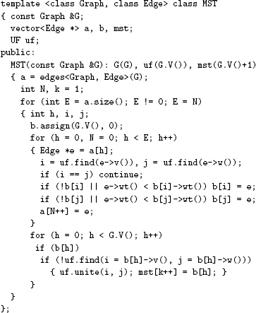
As we mentioned, Boruvka’s is the oldest of the algorithms that we consider: It was originally conceived in 1926, for a power-distribution application. The method was rediscovered by Sollin in 1961; it later attracted attention as the basis for MST algorithms with efficient asymptotic performance and as the basis for parallel MST algorithms.
Exercises
• 20.61 Show, in the style of Figure 20.14, the result of computing the MST of the network defined in Exercise 20.26 with Boruvka’s algorithm.
• 20.62 Why does Program 20.9 do a find test before doing the union operation? Hint: Consider equal-length edges.
• 20.63 Explain why b(h) could be null in the test in Program 20.9 that guards the union operation.
• 20.64 Describe a family of graphs with V vertices and E edges for which the number of edges that survive each stage of Boruvka’s algorithm is sufficiently large that the worst-case running time is achieved.
20.65 Develop an implementation of Boruvka’s algorithm that is based on a presorting of the edges.
• 20.66 Develop an implementation of Boruvka’s algorithm that uses doubly-linked circular lists to represent MST subtrees, so that subtrees can be merged and renamed in time proportional to E during each stage (and the equivalence-relations ADT is therefore not needed).
• 20.67 Do empirical studies to compare your implementation of Boruvka’s algorithm in Exercise 20.66 with the implementation in the text (Program 20.9), for various weighted graphs (see Exercises 20.9–14).
• 20.68 Do empirical studies to tabulate the number of stages and the number of edges processed per stage in Boruvka’s algorithm, for various weighted graphs (see Exercises 20.9–14).
20.69 Develop an implementation of Boruvka’s algorithm that constructs a new graph (one vertex for each tree in the forest) at each stage.
• 20.70 Write a client program that does dynamic graphical animations of Boruvka’s algorithm (see Exercises 20.52 and 20.60). Test your program on random Euclidean neighbor graphs and on grid graphs (see Exercises 20.17 and 20.19), using as many points as you can process in a reasonable amount of time.
Figure 20.16 Boruvka’s MST algorithm
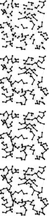
The MST evolves in just four stages for this example (top to bottom).
20.6 Comparisons and Improvements
Table 20.1 summarizes the running times of the basic MST algorithms that we have considered; Table 20.2 presents the results of an empirical study comparing the algorithms. From these tables, we can conclude that the adjacency-matrix implementation of Prim’s algorithm is the method of choice for dense graphs, that all the other methods perform within a small constant factor of the best possible (the time that it takes to extract the edges) for graphs of intermediate density, and that Kruskal’s method essentially reduces the problem to sorting for sparse graphs.
In short, we might consider the MST problem to be “solved” for practical purposes. For most graphs, the cost of finding the MST is only slightly higher than the cost of extracting the graph’s edges. This rule holds except for huge graphs that are extremely sparse, but the available performance improvement over the best known algorithms even in this case is approximately a factor of 10 at best. The results in Table 20.2 are dependent on the model used to generate graphs, but they are borne out for many other graph models as well (see, for example, Exercise 20.80). Still, the theoretical results do not deny the existence of an algorithm that is guaranteed to run in linear time for all graphs; here we take a look at the extensive research on improved implementations of these methods.
First, much research has gone into developing better priority-queue implementations. The Fibonacci heap data structure, an extension of the binomial queue, achieves the theoretically optimal performance of taking constant time for decrease key operations and logarithmic time for remove the minimum operations, which behavior translates, by Property 20.8, to a running time proportional to E + V lg V for Prim’s algorithm. Fibonacci heaps are more complicated than binomial queues and are somewhat unwieldy in practice, but some simpler priority-queue implementations have similar performance characteristics ( see reference section ).
One effective approach is to use radix methods for the priority-queue implementation. Performance of such methods is typically equivalent to that of radix sorting for Kruskal’s method, or even to that of using a radix quicksort for the partial-sorting method that we discussed in Section 20.4.
Another simple early approach, proposed by D. Johnson in 1977, is one of the most effective: Implement the priority queue for Prim’s algorithm with d -ary heaps, instead of with standard binary heaps (see Figure 20.17). Program 20.10 is a complete implementation of the priority-queue interface that we have been using that is based on this method. For this priority-queue implementation, decrease key takes less than logd V steps, and remove the minimum takes time proportional to d logd V. By Property 20.8, this behavior leads to a running time proportional to Vd logd V + E logd V for Prim’s algorithm, which is linear for graphs that are not sparse.
Table 20.1 Cost of MST algorithms
This table summarizes the cost (worst-case running time) of various MST algorithms considered in this chapter. The formulas are based on the assumptions that an MST exists (which implies that E V 1) and that there are X edges not longer than the longest edge in the MST − (see Property 20.10). These worst-case bounds may be too conservative to be useful in predicting performance on real graphs. The algorithms run in near-linear time in a broad variety of practical situations.
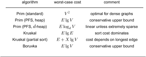
Property 20.12 Given a graph with V vertices and E edges, let d denote the density E/V. If d < 2 , then the running time of Prim’s algorithm is proportional to V lg V. Otherwise, we can improve the worst-case running time by a factor of lg( E/V ) by using a E/V -ary heap for the priority queue.
Proof: Continuing the discussion in the previous paragraph, the number of steps is Vd logd V + E logd V, so the running time is at most proportional to E logd V =( E lg V ) / lg d.
When E is proportional to V1+ [epsilon1], Property 20.12 leads to a worst-case running time proportional to E/[epsilon1], and that value is linear for any constant [epsilon1]. For example, if the number of edges is proportional to V3 / 2, the cost is less than 2 E; if the number of edges is proportional to
Table 20.2 Empirical study of MST algorithms
This table shows relative timings for various algorithms for finding the MST, for random weighted graphs of various density. For low densities, Kruskal’s algorithm is best because it amounts to a fast sort. For high densities, the classical implementation of Prim’s algorithm is best because it does not incur list-processing overhead. For intermediate densities, the PFS implementation of Prim’s algorithm runs within a small factor of the time that it takes to examine each graph edge.
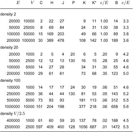
Key:
C extract edges only
H Prim’s algorithm (adjacency lists/indexed heap)
J Johnson’s version of Prim’s algorithm (d-heap priority queue)
P Prim’s algorithm (adjacency-matrix representation)
K Kruskal’s algorithm
K* Partial-sort version of Kruskal’s algorithm
B Boruvka’s algorithm
e edges examined (union operations)
V4 / 3, the cost is less than 3 E; and if the number of edges is proportional to V5 / 4, the cost is less than 4 E. For a graph with 1 million vertices, the cost is less than 6 E unless the density is less than 10.
The temptation to minimize the bound on the worst-case running time in this way needs to be tempered with the realization that the Vd logd V part of the cost is not likely to be avoided (for remove the minimum, we have to examine d successors in the heap as we sift down), but the E lg d part is not likely to be achieved (since most edges will not require a priority-queue update, as we showed in the discussion following Property 20.8).
For typical graphs such as those in the experiments in Table 20.2, decreasing d has no effect on the running time, and using a large value of d can slow down the implementation slightly. Still, the slight protection offered for worst-case performance makes the method worthwhile since it is so easy to implement. In principle, we could tune the implementation to pick the best value of d for certain types of graphs (choose the largest value that does not slow down the algorithm), but a small fixed value (such as 4, 5, or 6) will be fine except possibly for some particular huge classes of graphs that have atypical characteristics.
Using d -heaps is not effective for sparse graphs because d has to be an integer greater than or equal to 2, a condition that implies that we cannot bring the asymptotic running time lower than V lg V. Ifthe density is a small constant, then a linear-time MST algorithm would have to run in time proportional to V.
The goal of developing practical algorithms for computing the MST of sparse graphs in linear time remains elusive. A great deal of research has been done on variations of Boruvka’s algorithm as the basis for nearly linear-time MST algorithms for extremely sparse graphs ( see reference section ). Such research still holds the potential to lead us eventually to a practical linear-time MST algorithm and has even shown the existence of a randomized linear-time algorithm. While these algorithms are generally quite complicated, simplified versions of some of them may yet be shown to be useful in practice. In the meantime, we can use the basic algorithms that we have considered here to compute the MST in linear time in most practical situations, perhaps paying an extra factor of lg V for some sparse graphs.
Figure 20.17 2-, 3-, and 4-ary heaps
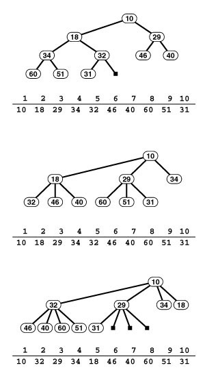
When we store a standard binary heap-ordered complete tree in an array (top), we use implicit links to take us from a node i down the tree to its children 2 i and 2 i + 1 and up the tree to its parent i/ 2. In a 3-ary heap (center), implicit links for i are to its children 3 i 1, 3 i, and 3 i + 1 and to its parent − [floorleft] ( i +1) / 3 [floorright]; and in a 4-ary heap (bottom), implicit links for i are to its children 4 i − 2, 4 i 1, 4 i, and 4 i +1 and to its parent −[floorleft] ( i +2) / 4. Increasing the branching factor in [floorright] an implicit heap implementation can be valuable in applications, like Prim’s algorithm, that require a significant number of decrease key operations.
Program 20.10 Multiway heap PQ implementation
This class uses multiway heaps to implement the indirect priority-queue interface that we use in this book. It is based on changing Program 9.12 to have the constructor take a reference to a vector of priorities, to implement getmin and lower instead of delmax and change, and to generalize fixUp and fixDown so that they maintain a d -way heap (so remove the minimum takes time proportional to d logd V, but decrease key requires less than logd V steps).
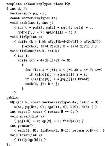
Exercises
• 20.71 [V. Vyssotsky] Develop an implementation of the algorithm discussed in Section 20.2 that builds the MST by adding edges one at a time and deleting the longest edges on the cycle formed (see Exercise 20.33). Use a parent-link representation of a forest of MST subtrees. Hint: Reverse pointers when traversing paths in trees.
• 20.72 Run empirical tests to compare the running time of your implementation in Exercise 20.71 with that of Kruskal’s algorithm, for various weighted graphs (see Exercises 20.9–14). Check whether randomizing the order in which the edges are considered affects your results.
• 20.73 Describe how you would find the MST of a graph so large that only V edges can fit into main memory at once.
• 20.74 Develop a priority-queue implementation for which remove the minimum and find the minimum are constant-time operations, and for which decrease key takes time proportional to the logarithm of the priority-queue size. Compare your implementation with 4-heaps when you use Prim’s algorithm to find the MST of sparse graphs, for various weighted graphs (see Exercises 20.9–14).
20.75 Run empirical studies to compare the performance of various priority-queue implementations when used in Prim’s algorithm for various weighted graphs (see Exercises 20.9–14). Consider d -heaps for various values of d, binomial queues, the STL priority_queue, balanced trees, and any other data structure that you think might be effective.
20.76 Develop an implementation that generalizes Boruvka’s algorithm to maintain a generalized queue containing the forest of MST subtrees. (Using Program 20.9 corresponds to using a FIFO queue.) Experiment with other generalized-queue implementations, for various weighted graphs (see Exercises 20.9–14).
• 20.77 Develop a generator for random connected cubic graphs (each vertex of degree 3) that have random weights on the edges. Fine-tune for this case the MST algorithms that we have discussed, then determine which is the fastest.
• 20.78 For V = 106, plot the ratio of the upper bound on the cost for Prim’s algorithm with d -heaps to E as a function of the density d, for d in the range from 1 to 100.
• 20.79 Table 20.2 suggests that the standard implementation of Kruskal’s algorithm is significantly faster than the partial-sort implementation for low-density graphs. Explain this phenomenon.
• 20.80 Run an empirical study, in the style of Table 20.2, for random complete graphs that have Gaussian weights (see Exercise 20.18).
20.7 Euclidean MST
Suppose that we are given N points in the plane and we want to find the shortest set of lines connecting all the points. This geometric problem is called the Euclidean MST problem (see Figure 20.18). One way to solve it is to build a complete graph with N vertices and N ( N−1) / 2 edges—one edge connecting each pair of vertices weighted with the distance between the corresponding points. Then, we can use Prim’s algorithm to find the MST in time proportional to N 2.
This solution is generally too slow. The Euclidean problem is somewhat different from the graph problems that we have been considering because all the edges are implicitly defined. The size of the input is just proportional to N, so the solution that we have sketched is a quadratic algorithm for the problem. Research has proved that it is possible to do better. The geometric structure makes most of the edges in the complete graph irrelevant to the problem, and we do not need to add most of them to the graph before we construct the minimum spanning tree.
Property 20.13 We can find the Euclidean MST of N points in time proportional to N log N.
This fact is a direct consequence of two basic facts about points in the plane that we discuss in detail in Part 7. First, a graph known as the Delauney triangulation contains the MST, by definition. Second, the Delauney triangulation is a planar graph whose number of edges is proportional to N.
In principle, then, we could compute the Delauney triangulation in time proportional to N log N, then run either Kruskal’s algorithm or the priority-first search method to find the Euclidean MST, in time proportional to N log N. But writing a program to compute the Delauney triangulation is a challenge for even an experienced programmer, so this approach may be overkill for this problem in practice.
Figure 20.18 Euclidean MST
Given a set of N points in the plane (top), the Euclidean MST is the shortest set of lines connecting them together (bottom). This problem is not just a graph-processing problem, because we need to make use of global geometric information about the points to avoid having to process all N 2 implicit edges connecting the points.
Other approaches derive from the geometric algorithms that we consider in Part 7. For randomly distributed points, we can divide up the plane into squares such that each square is likely to contain about lg N/ 2 points, as we did for the closest-point computation in Program 3.20. Then, even if we include in the graph only the edges connecting each point to the points in the neighboring squares, we are likely (but are not guaranteed) to get all the edges in the minimum spanning tree; in that case, we could use Kruskal’s algorithm or the PFS implementation of Prim’s algorithm to finish the job efficiently. The example that we have used in Figure 20.10,Figure 20.13,Figure 20.16 and similar figures was created in this way (see Figure 20.19). Or, we could develop a version of Prim’s algorithm based on using near-neighbor algorithms to avoid updating distant vertices.
With all the possible choices that we have for approaching this problem and with the possibility of linear algorithms for the general MST problem, it is important to note that there is a simple lower bound on the best that we could do.
Property 20.14 Finding the Euclidean MST of N points is no easier than sorting N numbers.
Proof: Given a list of numbers to be sorted, convert the list into a list of points where the x coordinate is taken from the corresponding number of the list and the y coordinate is 0. Find the MST of that list of points. Then (as we did for Kruskal’s algorithm), put the points into a graph ADT and run DFS to produce a spanning tree, starting at the point with the lowest x coordinate. That spanning tree amounts to a linked-list sort of the numbers in order; thus, we have solved the sorting problem.
Precise interpretations of this lower bound are complicated because the basic operations used for the two problems (comparisons of coordinates for the sorting problem, distances for the MST problem) are different and because there is a possibility of using methods such as radix sort and grid methods. However, we may interpret the bound to mean that, as we do sorting, we should consider a Euclidean MST algorithm that uses N lg N comparisons to be optimal unless we exploit numerical properties of the coordinates, in which case we might expect to it to be linear time ( see reference section ).
Figure 20.19 Euclidean near-neighbor graphs
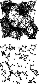
One way to compute the Euclidean MST is to generate a graph with edges connecting every pair of points within a distance d, as in the graph in Figure 20.8 et al. However, this method yields too many edges if d is too large (top) and is not guaranteed to have edges connecting all the points if d is smaller than the longest edge in the MST (bottom).
It is interesting to reflect on the relationship between graph and geometric algorithms that is brought out by the Euclidean MST problem. Many of the practical problems that we might encounter could be formulated either as geometric problems or as graph problems. If the physical placement of objects is a dominating characteristic, then the geometric algorithms of Part 7 may be called for; but if interconnections between objects are of fundamental importance, then the graph algorithms of this section may be better.
The Euclidean MST seems to fall at the interface between these two approaches (the input involves geometry and the output involves interconnections), and the development of simple, straightforward methods for the Euclidean MST remains an elusive goal. In Chapter 21, we see a similar problem that falls at this interface, but where a Euclidean approach admits substantially faster algorithms than do the corresponding graph problems.
Exercises
• 20.81 Give a counterexample to show why the following method for finding the Euclidean MST does not work: “Sort the points on their x coordinates, then find the minimum spanning trees of the first half and the second half, then find the shortest edge that connects them.”
• 20.82 Develop a fast version of Prim’s algorithm for computing the Euclidean MST of a uniformly distributed set of points in the plane based on ignoring distant points until the tree approaches them.
•• 20.83 Develop an algorithm that, given a set of N points in the plane, finds a set of edges of cardinality proportional to N that is certain to contain the MST and is sufficiently easy to compute that you can develop a concise and efficient implementation of your algorithm.
• 20.84 Given a random set of N points in the unit square (uniformly distributed), empirically determine a value of d, to within two decimal places, such that the set of edges defined by all pairs of points within distance d of one another is 99 percent certain to contain the MST.
• 20.85 Work Exercise 20.84 for points where each coordinate is drawn from a Gaussian distribution with mean 0.5 and standard deviation 0.1.
• 20.86 Describe how you would improve the performance of Kruskal’s and Boruvka’s algorithm for sparse Euclidean graphs.