
CHAPTER EIGHTEEN
Graph Search
WE OFTEN LEARN properties of a graph by systematically examining each of its vertices and each of its edges. Determining some simple graph properties—for example, computing the degrees of all the vertices—is easy if we just examine each edge (in any order whatever). Many other graph properties are related to paths, so a natural way to learn them is to move from vertex to vertex along the graph’s edges. Nearly all the graph-processing algorithms that we consider use this basic abstract model. In this chapter, we consider the fundamental graph-search algorithms that we use to move through graphs, learning their structural properties as we go.
Graph searching in this way is equivalent to exploring a maze. Specifically, passages in the maze correspond to edges in the graph, and points where passages intersect in the maze correspond to vertices in the graph. When a program changes the value of a variable from vertex v to vertex w because of an edge v-w, we view it as equivalent to a person in a maze moving from point v to point w. We begin this chapter by examining a systematic exploration of a maze. By correspondence with this process, we see precisely how the basic graph-search algorithms proceed through every edge and every vertex in a graph.
In particular, the recursive depth-first search (DFS) algorithm corresponds precisely to the particular maze-exploration strategy of Section 18.1. DFS is a classic and versatile algorithm that we use to solve connectivity and numerous other graph-processing problems. The basic algorithm admits two simple implementations: one that is recursive, and another that uses an explicit stack. Replacing the stack with a FIFO queue leads to another classic algorithm,breadth-first search (BFS), which we use to solve another class of graph-processing problems related to shortest paths.
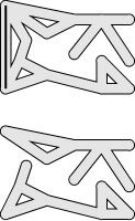
Figure 18.1 Exploring a maze

We can explore every passageway in a simple maze by following a simple rule such as “keep your right hand on the wall.” Following this rule in the maze at the top, we explore the whole maze, going through each passage once in each direction. But if we follow this rule in a maze with a cycle, we return to the starting point without exploring the whole maze, as illustrated in the maze at the bottom.
The main topics of this chapter are DFS, BFS, their related algorithms, and their application to graph processing. We briefly considered DFS and BFS in Chapter 5; we treat them from first principles here, in the context of search-based graph-processing classes, and use them to demonstrate relationships among various graph algorithms. In particular, we consider a general approach to searching graphs that encompasses a number of classical graph-processing algorithms, including both DFS and BFS.
As illustrations of the application of these basic graph-searching methods to solve more complicated problems, we consider algorithms for finding connected components, biconnected components, spanning trees, and shortest paths, and for solving numerous other graph-processing problems. These implementations exemplify the approach that we shall use to solve more difficult problems in Chapters 19 through 22.
We conclude the chapter by considering the basic issues involved in the analysis of graph algorithms, in the context of a case study comparing several different algorithms for finding the number of connected components in a graph.
18.1 Exploring a Maze
It is instructive to think about the process of searching through a graph in terms of an equivalent problem that has a long and distinguished history (see reference section)—finding our way through a maze that consists of passages connected by intersections. This section presents a detailed study of a basic method for exploring every passage in any given maze. Some mazes can be handled with a simple rule, but most mazes require a more sophisticated strategy (see Figure 18.1). Using the terminology maze instead of graph,passage instead of edge, and intersection instead of vertex is making mere semantic distinctions, but, for the moment, doing so will help to give us an intuitive feel for the problem.
One trick for exploring a maze without getting lost that has been known since antiquity (dating back at least to the legend of Theseus and the Minotaur) is to unroll a ball of string behind us. The string guarantees that we can always find a way out, but we are also interested in being sure that we have explored every part of the maze, and we do not want to retrace our steps unless we have to. To accomplish these goals, we need some way to mark places that we have been. We could use the string for this purpose as well, but we use an alternative approach that models a computer implementation more closely.
We assume that there are lights, initially off, in every intersection, and doors, initially closed, at both ends of every passage. We further assume that the doors have windows and that the lights are sufficiently strong and the passages sufficiently straight that we can determine, by opening the door at one end of a passage, whether or not the intersection at the other end is lit (even if the door at the other end is closed). Our goals are to turn on all the lights and to open all the doors. To reach them, we need a set of rules to follow, systematically. The following maze-exploration strategy, which we refer to as Trémaux exploration, has been known at least since the nineteenth century (see reference section):
(i) If there are no closed doors at the current intersection, go to step (iii). Otherwise, open any closed door to any passage leading out of the current intersection (and leave it open).
(ii) If you can see that the intersection at the other end of that passage is already lighted, try another door at the current intersection (step (i)). Otherwise (if you can see that the intersection at the other end of the passage is dark), follow the passage to that intersection, unrolling the string as you go, turn on the light, and go to step (i).
(iii) If all the doors at the current intersection are open, check whether you are back at the start point. If so, stop. If not, use the string to go back down the passage that brought you to this intersection for the first time, rolling the string back up as you go, and look for another closed door there (that is, return to step (i)).
Figures 18.2 and 18.3 depict a traversal of a sample graph and show that, indeed, every light is lit and every door is opened for that example. The figures depict just one of many possible outcomes of the exploration, because we are free to open the doors in any order at each intersection. Convincing ourselves that this method is always effective is an interesting exercise in mathematical induction.
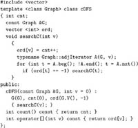
Figure 18.2 Trémaux maze exploration example
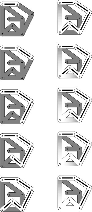
In this diagram, places that we have not visited are shaded (dark) and places that we have visited are white (light). We assume that there are lights in the intersections, and that, when we have opened doors into lighted intersections on both ends of a passage, the passage is lighted. To explore the maze, we begin at 0 and take the passage to 2 (left, top). Then we proceed to 6, 4, 3, and 5, opening the doors to the passages, lighting the intersections as we proceed through them, and leaving a string trailing behind us (left). When we open the door that leads to 0 from 5, we can see that 0 is lighted, so we skip that passage (top right). Similarly, we skip the passage from 5 to 4 (right, second from top), leaving us with nowhere to go from 5 except back to 3 and then back to 4, rolling up our ball of string. When we open the doorway from the passage from 4 to 5, we can see that 5 is lighted through the open door at the other end, and we therefore skip that passage (right, bottom). We never walked down the passage connecting 4 and 5, but we lighted it by opening the doors at both ends.
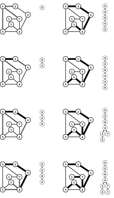
Figure 18.3 Trémaux maze exploration example (continued)
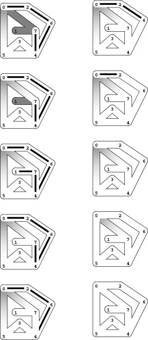
Next, we proceed to 7 (top left), open the door to see that 0 is lighted (left, second from top), and then proceed to 1 (left, third from top). At this point, most of the maze is traversed, and we use our string to take us back to the beginning, moving from 1 to 7 to 4 to 6 to 2 to 0. Back at 0, we complete our exploration by checking the passages to 5 (right, second from bottom) and 7 (bottom right), leaving all passages and intersections lighted. Again, the passages connecting 0 to 5 and 0 to 7 are both lighted because we opened the doors at both ends, but we did not walk through them.
Figure 18.4 Decomposing a maze
To prove by induction that Trémaux exploration takes us everywhere in a maze (top), we break it into two smaller pieces, by removing all edges connecting the first intersection with any intersection that can be reached from the first passage without going back through the first intersection (bottom).
Property 18.1 When we use Trémaux maze exploration, we light all lights and open all doors in the maze and end up back where we started.
Proof: To prove this assertion by induction, we first note that it holds, trivially, for a maze that contains one intersection and no passages—we just turn on the light. For any maze that contains more than one intersection, we assume the property to be true for all mazes with fewer intersections. It suffices to show that we visit all intersections, since we open all the doors at every intersection that we visit. Now, consider the first passage that we take from the first intersection, and divide the intersections into two subsets: (i) those that we can reach by taking that passage without returning to the start, and (ii) those that we cannot reach from that passage without returning to the start. Applying the inductive hypothesis, we know that we visit all intersections in (i) (ignoring any passages back to the start intersection, which is lit) and end up back at the start intersection. Then, applying the the inductive hypothesis again, we know that we visit all intersections in (ii) (ignoring the passages from the start to intersections in (i), which are lit). •
From the detailed example in Figures 18.2 and 18.3, we see that there are four different possible situations that arise for each passage that we consider taking:
(i) The passage is dark, so we take it.
(ii) The passage is the one that we used to enter (it has our string in it), so we use it to exit (and we roll up the string).
(iii) The door at the other end of the passage is closed (but the intersection is lit), so we skip the passage.
(iv) The door at the other end of the passage is open (and the intersection is lit), so we skip it.
The first and second situations apply to any passage that we traverse, first at one end and then at the other end. The third and fourth situations apply to any passage that we skip, first at one end and then at the other end. Next, we see how this perspective on maze exploration translates directly to graph search.
Exercises
• 18.1 Assume that intersections 6 and 7 (and all the hallways connected to them) are removed from the maze in Figures 18.2 and 18.3, and a hallway is added that connects 1 and 2. Show a Trémaux exploration of the resulting maze, in the style of Figures 18.2 and 18.3.
• 18.2 Which of the following could not be the order in which lights are turned on at the intersections during a Trémaux exploration of the maze depicted in Figures 18.2 and 18.3?
0-7-4-5-3-1-6-2
0-2-6-4-3-7-1-5
0-5-3-4-7-1-6-2
0-7-4-6-2-1-3-5
• 18.3 How many different ways are there to traverse the maze depicted in Figures 18.2 and 18.3 with a Trémaux exploration?
18.2 Depth-First Search
Our interest in Trémaux exploration is that this technique leads us immediately to the classic recursive function for traversing graphs: To visit a vertex, we mark it as having been visited, then (recursively) visit all the vertices that are adjacent to it and that have not yet been marked. This method, which we considered briefly in Chapters 3 and 5 and used to solve path problems in Section 17.7, is called depth-first search (DFS). It is one of the most important algorithms that we shall encounter. DFS is deceptively simple because it is based on a familiar concept and is easy to implement; in fact, it is a subtle and powerful algorithm that we put to use for numerous difficult graph-processing tasks.
Program 18.1 is a DFS class that visits all the vertices and examines all the edges in a connected graph. Like the simple path-search functions that we considered in Section 17.7, it is based on a recursive function that keeps a private vector to mark vertices as having been visited. In this implementation, ord is a vector of integers that records the order in which vertices are visited. Figure 18.5 is a trace that shows the order in which Program 18.1 visits the edges and vertices for the example depicted in Figures 18.2 and 18.3 (see also Figure 18.17), when the adjacency-matrix graph implementation DenseGRAPH of Section 17.3 is used. Figure 18.6 depicts the maze-exploration process using standard graph drawings.
These figures illustrate the dynamics of a recursive DFS and show the correspondence with Trémaux exploration of a maze. First, the vertex-indexed vector corresponds to the lights in the intersections: When we encounter an edge to a vertex that we have already visited (see a light at the end of the passage), we do not make a recursive
Figure 18.5 DFS trace
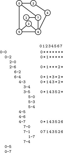
This trace shows the order in which DFS checks the edges and vertices for the adjacency-matrix representation of the graph corresponding to the example in Figures 18.2 and 18.3 (top) and traces the contents of the ord vector (right) as the search progresses (asterisks represent -1, for unseen vertices). There are two lines in the trace for every graph edge (once for each orientation). Indentation indicates the level of recursion.
Program 18.1 Depth-first search of a connected component
This DFS class corresponds to Trémaux exploration. The constructor marks as visited all vertices in the same connected component as v by calling the recursive searchC, which visits all the vertices adjacent to v by checking them all and calling itself for each edge that leads from v to an unmarked vertex. Clients can use the count function to learn the number of vertices encountered and the overloaded [] operator to learn the order in which the search visited the vertices.
call to follow that edge (go down that passage). Second, the function call–return mechanism in the program corresponds to the string in the maze: When we have processed all the edges adjacent to a vertex (explored all the passages leaving an intersection), we “return” (in both senses of the word).
In the same way that we encounter each passage in the maze twice (once at each end), we encounter each edge in the graph twice (once at each of its vertices). In Trémaux exploration, we open the doors at each end of each passage; in DFS of an undirected graph, we
Figure 18.6 Depth-first search
These diagrams are a graphical view of the process depicted in Figure 18.5, showing the DFS recursive-call tree as it evolves. Thick black edges in the graph correspond to edges in the DFS tree shown to the right of each graph diagram. Shaded edges are the candidates to be added to the tree next. In the early stages (left) the tree grows down in a straight line, as we make recursive calls for 0, 2, 6, and 4 (left). Then we make recursive calls for 3, then 5 (right, top two diagrams); and return from those calls to make a recursive call for 7 from 4 (right, second from bottom) and to 1 from 7 (right, bottom).
Figure 18.7 DFS trace (adjacency lists)
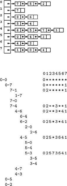
This trace shows the order in which DFS checks the edges and vertices for the adjacency-lists representation of the same graph as in Figure 18.5.
check each of the two representations of each edge. If we encounter an edge v-w, we either do a recursive call (if w is not marked) or skip the edge (if w is marked). The second time that we encounter the edge, in the opposite orientation w-v, we always ignore it, because the destination vertex v has certainly already been visited (the first time that we encountered the edge).
One difference between DFS as implemented in Program 18.1 and Trémaux exploration as depicted in Figures 18.2 and 18.3, although it is inconsequential in many contexts, is worth taking the time to understand. When we move from vertex v to vertex w, we have not examined any of the entries in the adjacency matrix that correspond to edges from w to other vertices in the graph. In particular, we know that there is an edge from w to v and that we will ignore that edge when we get to it (because v is marked as visited). That decision happens at a time different from in the Trémaux exploration, where we open the doors corresponding to the edge from v to w when we go to w for the first time, from v. If we were to close those doors on the way in and open them on the way out (having identified the passage with the string), then we would have a precise correspondence between DFS and Trémaux exploration.
Figure 18.6 also depicts the tree corresponding to the recursive calls as it evolves, in correspondence with Figure 18.5. This recursive-call tree, which is known as the DFS tree, is a structural description of the search process. As we see in Section 18.4, the DFS tree, properly augmented, can provide a full description of the search dynamics, in addition to just the call structure.
The order in which vertices are visited depends not just on the graph, but on its representation and ADT implementation. For example, Figure 18.7 shows the search dynamic when the SparseMultiGRAPH adjacency-lists implementation of Section 17.4 is used. For the adjacency-matrix representation, we examine the edges incident on each vertex in numerical order; for the adjacency-lists representation, we examine them in the order that they appear on the lists. This difference leads to a completely different recursive search dynamic, as would differences in the order in which edges appear on the lists (which occur, for example, when the same graph is constructed by inserting edges in a different order). Note also that the existence of parallel edges is inconsequential for DFS because any edge that is parallel to an edge that has already been traversed is ignored, since its destination vertex has been visited.
Despite all of these possibilities, the critical fact remains that DFS visits all the edges and all the vertices connected to the start vertex, regardless of in what order it examines the edges incident on each vertex. This fact is a direct consequence of Property 18.1, since the proof of that property does not depend on the order in which the doors are opened at any given intersection. All the DFS-based algorithms that we examine have this same essential property. Although the dynamics of their operation might vary substantially depending on the graph representation and details of the implementation of the search, the recursive structure gives us a way to make relevant inferences about the graph itself, no matter how it is represented and no matter which order we choose to examine the edges incident upon each vertex.
Exercises
• 18.4 Add a public member function to Program 18.1 that returns the size of the connected component searched by the constructor.
18.5 Write a client program like Program 17.6 that scans a graph from standard input, uses Program 18.1 to run a search starting at each vertex, and prints out the parent-link representation of each spanning forest. Use the DenseGRAPH graph ADT implementation from Section 17.3.
• 18.6 Show, in the style of Figure 18.5, a trace of the recursive function calls made when a cDFS<DenseGRAPH> object is constructed for the graph
0-2 0-5 1-2 3-4 4-5 3-5.
Draw the corresponding DFS recursive-call tree.
18.7 Show, in the style of Figure 18.6, the progress of the search for the example in Exercise 18.6.
18.3 Graph-Search ADT Functions
DFS and the other graph-search methods that we consider later in this chapter all involve following graph edges from vertex to vertex, with the goal of systematically visiting every vertex and every edge in the graph. But following graph edges from vertex to vertex can lead us to all the vertices in only the same connected component as the starting vertex. In general, of course, graphs might not be connected, so we need one call on a search function for each connected component. We
will typically use graph-search functions that perform the following steps until all of the vertices of the graph have been marked as having been visited:
• Find an unmarked vertex (a start vertex).
• Visit (and mark as visited) all the vertices in the connected component that contains the start vertex.
The method for marking vertices is not specified in this description, but we most often use the same method that we used for the DFS implementations in Section 18.2: We initialize all entries in a private vertex-indexed vector to a negative integer, and mark vertices by setting their corresponding entry to a nonnegative value. Using this procedure amounts to using a single bit (the sign bit) for the mark; most implementations are also concerned with keeping other information associated with marked vertices in the vector (such as, for the DFS implementation in Section 18.2, the order in which vertices are marked). The method for looking for a vertex in the next connected component is also not specified, but we most often use a scan through the vector in order of increasing index.
We pass an edge to the search function (using a dummy self-loop in the first call for each connected component), instead of passing its destination vertex, because the edge tells us how we reached the vertex. Knowing the edge corresponds to knowing which passage led to a particular intersection in a maze. This information is useful in many DFS classes. When we are simply keeping track of which vertices we have visited, this information is of little consequence; but more interesting problems require that we always know from whence we came.
Program 18.2 is an implementation that illustrates these choices. Figure 18.8 gives an example that illustrates how every vertex is visited, by the effect on the ord vector of any derived class. Typically, the derived classes that we consider also examine all edges incident upon each vertex visited. In such cases, knowing that we visit all vertices tells us that we visit all edges as well, as in Trémaux traversal.
Program 18.3 is an example that shows how we derive a DFS-based class for computing a spanning forest from the SEARCH base class of Program 18.2. We include a private vector st in the derived class to hold a parent-link representation of the tree that we initialize in the constructor; define a searchC that is similar to searchC from Program 18.1, except that it takes an edge v-w as argument and to set st[w] to v; and add a public member function that allows clients to learn the parent of any vertex. Spanning forests are of interest in many applications, but our primary interest in them in this chapter is their relevance in understanding the dynamic behavior of the DFS, the topic of Section 18.4.
In a connected graph, the constructor in Program 18.2 calls searchC once for 0-0 and then finds that all the other vertices are marked. In a graph with more than one connected component, the constructor checks all the connected components in a straightforward manner. DFS is the first of several methods that we consider for searching a connected component. No matter which method (and no matter what graph representation) we use, Program 18.2 is an effective method for visiting all the graph vertices.
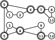
Figure 18.8 Graph search
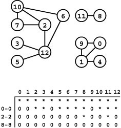
The table at the bottom shows vertex marks (contents of the ord vector) during a typical search of the graph at the top. Initially, the function GRAPHsearch in Program 18.2 unmarks all vertices by setting the marks all to -1 (indicated by an asterisk). Then it calls search for the dummy edge 0-0, which marks all of the vertices in the same connected component as 0 (second row) by setting them to a nonnegative values (indicated by 0s). In this example, it marks 0, 1, 4, and 9 with the values 0 through 3 in that order. Next, it scans from left to right to find the unmarked vertex 2 and calls search for the dummy edge 2-2 (third row), which marks the seven vertices in the same connected component as 2. Continuing the left-to-right scan, it calls search for 8-8 to mark 8 and 11 (bottom row). Finally, GRAPHsearch completes the search by discovering that 9 through 12 are all marked.
Property 18.2 A graph-search function checks each edge and marks each vertex in a graph if and only if the search function that it uses marks each vertex and checks each edge in the connected component that contains the start vertex.
Proof: By induction on the number of connected components. •
Graph-search functions provide a systematic way of processing each vertex and each edge in a graph. Generally, our implementations are designed to run in linear or near-linear time, by doing a fixed amount of processing per edge. We prove this fact now for DFS, noting that the same proof technique works for several other search strategies.
Property 18.3 DFS of a graph represented with an adjacency matrix requires time proportional to V2.
Proof: An argument similar to the proof of Property 18.1 shows that searchC not only marks all vertices connected to the start vertex but also calls itself exactly once for each such vertex (to mark that vertex). An argument similar to the proof of Property 18.2 shows that a call to search leads to exactly one call to searchC for each graph vertex. In searchC, the iterator checks every entry in the vertex’s row in the adjacency matrix. In other words, the search checks each entry in the adjacency matrix precisely once.•
Property 18.4 DFS of a graph represented with adjacency lists requires time proportional to V + E.
Proof: From the argument just outlined, it follows that we call the recursive function precisely V times (hence the V term), and we examine each entry on each adjacency list (hence the E term).•
The primary implication of Properties 18.3 and 18.4 is that they establish the running time of DFS to be linear in the size of the data structure used to represent the graph. In most situations, we are also justified in thinking of the running time of DFS as being linear in the size of the graph, as well: If we have a dense graph (with the number of edges proportional to V2) then either representation gives this result; if we have a sparse graph, then we assume use of an adjacency-lists representation. Indeed, we normally think of the running time of DFS as being linear in E. That statement is technically not true if we are using adjacency matrices for sparse graphs or for extremely sparse graphs with E << V and most vertices isolated, but we can usually avoid the former situation, and we can remove isolated vertices (see Exercise 17.34) in the latter situation.
As we shall see, these arguments all apply to any algorithm that has a few of the same essential features of DFS. If the algorithm marks each vertex and examines all the latter’s incident vertices (and does any other work that takes time per vertex bounded by a constant), then these properties apply. More generally, if the time per vertex is bounded by some function f (V, E), then the time for the search is guaranteed to be proportional to E + Vf (V, E). In Section 18.8, we see that DFS is one of a family of algorithms that has just these characteristics; in Chapters 19 through 22, we see that algorithms from this family serve as the basis for a substantial fraction of the code that we consider in this book.
Much of the graph-processing code that we examine is ADT-implementation code for some particular task, where we develop a class that does a basic search to compute structural information in other vertex-indexed vectors. We can derive the class from Program 18.2 or, in simple cases, just reimplement the search. Many of our graph-processing classes are of this nature because we typically can uncover a graph’s structure by searching it. We normally add code to the search function that is executed when each vertex is marked, instead of working with a more generic search (for example, one that calls a specified function each time a vertex is visited), solely to keep the code compact and self-contained. Providing a more general ADT mechanism for clients to process all the vertices with a client-supplied function is a worthwhile exercise (see Exercises 18.13 and 18.14).
In Sections 18.5 and 18.6, we examine numerous graph-processing functions that are based on DFS. In Sections 18.7 and 18.8, we look at other implementations of search and at some graph-processing functions that are based on them. Although we do not build this layer of abstraction into our code, we take care to identify the basic graph-search strategy underlying each algorithm that we develop. For example, we use the term DFS class to refer to any implementation that is based on the recursive DFS scheme. The simple-path–search class Program 17.11 and the spanning-forest class Program 18.3 are examples of DFS classes.
Many graph-processing functions are based on the use of vertex-indexed vectors. We typically include such vectors as private data members in class implementations, to hold information about the structure of graphs (which is discovered during the search) that helps us solve the problem at hand. Examples of such vectors are the deg vector in Program 17.11 and the ord vector in Program 18.1. Some implementations that we will examine use multiple vectors to learn complicated structural properties.
Our convention in graph-search functions is to initialize all entries in vertex-indexed vectors to -1, and to set the entries corresponding to each vertex visited to nonnegative values in the search function. Any such vector can play the role of the ord vector (marking vertices as visited) in Programs 18.2 through 18.3. When a graph-search function is based on using or computing a vertex-indexed vector, we often just implement the search and use that vector to mark vertices, rather than deriving the class from SEARCH or maintaining the ord vector.
The specific outcome of a graph search depends not just on the nature of the search function but also on the graph representation and even the order in which search examines the vertices. For specificity in the examples and exercises in this book, we use the term standard adjacency-lists DFS to refer to the process of inserting a sequence of edges into a graph ADT implemented with an adjacency-lists representation (Program 17.9), then doing a DFS with, for example, Program 18.3. For the adjacency-matrix representation, the order of edge insertion does not affect search dynamics, but we use the parallel term standard adjacency-matrix DFS to refer to the process of inserting a sequence of edges into a graph ADT implemented with an adjacency-matrix representation (Program 17.7), then doing a DFS with, for example, Program 18.3.
Exercises
18.8 Show, in the style of Figure 18.5, a trace of the recursive function calls made for a standard adjacency-matrix DFS of the graph
3-7 1-4 7-8 0-5 5-2 3-8 2-9 0-6 4-9 2-6 6-4.
18.9 Show, in the style of Figure 18.7, a trace of the recursive function calls made for a standard adjacency-lists DFS of the graph
3-7 1-4 7-8 0-5 5-2 3-8 2-9 0-6 4-9 2-6 6-4.
18.10 Modify the adjacency-matrix graph ADT implementation in Program 17.7 to use a dummy vertex that is connected to all the other vertices. Then, provide a simplified DFS implementation that takes advantage of this change.
18.11 Do Exercise 18.10 for the adjacency-lists ADT implementation in Program 17.9.
• 18.12 There are 13! different permutations of the vertices in the graph depicted in Figure 18.8. How many of these permutations could specify the order in which vertices are visited by Program 18.2?
18.13 Implement a graph ADT client function that calls a client-supplied function for each vertex in the graph.
18.14 Implement a graph ADT client that calls a client-supplied function for each edge in the graph. Such a function might be a reasonable alternative to GRAPHedges (see Program 17.2).
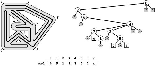
Figure 18.9 DFS tree representations
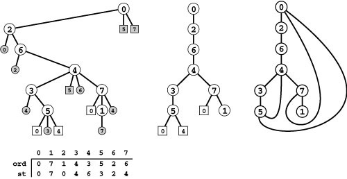
If we augment the DFS recursive-call tree to represent edges that are checked but not followed, we get a complete description of the DFS process (left). Each tree node has a child representing each of the nodes adjacent to it, in the order they were considered by the DFS, and a preorder traversal gives the same information as Figure 18.5: first we follow 0-0, then 0-2, then we skip 2-0, then we follow 2-6, then we skip 6-2, then we follow 6-4, then 4-3, and so forth. The ord vector specifies the order in which we visit tree vertices during this preorder walk, which is the same as the order in which we visit graph vertices in the DFS. The st vector is a parent-link representation of the DFS recursive-call tree (see Figure 18.6).
There are two links in the tree for every edge in the graph, one for each of the two times it encounters the edge. The first is to an unshaded node and either corresponds to making a recursive call (if it is to an internal node) or to skipping a recursive call because it goes to an ancestor for which a recursive call is in progress (if it is to an external node). The second is to a shaded external node and always corresponds to skipping a recursive call, either because it goes back to the parent (circles) or because it goes to a descendent of the parent for which a recursive call is in progress (squares). If we eliminate shaded nodes (center), then replace the external nodes with edges, we get another drawing of the graph (right).
18.4 Properties of DFS Forests
As noted in Section 18.2, the trees that describe the recursive structure of DFS function calls give us the key to understanding how DFS operates. In this section, we examine properties of the algorithm by examining properties of DFS trees.
If we add external nodes to the DFS tree to record the moments when we skipped recursive calls for vertices that had already been visited, we get the compact representation of the dynamics of DFS illustrated in Figure 18.9. This representation is worthy of careful study. The tree is a representation of the graph, with a vertex corresponding to each graph vertex and an edge corresponding to each graph edge. We can choose to show the two representations of the edge that we process (one in each direction), as shown in the left part of the figure, or just one representation of each edge, as shown in the center and right parts of the figure. The former is useful in understanding that the algorithm processes each and every edge; the latter is useful in understanding that the DFS tree is simply another graph representation. Traversing the internal nodes of the tree in preorder gives the vertices in the order in which DFS visits them; moreover, the order in which we visit the edges of the tree as we traverse it in preorder is the same as the order in which DFS examines the edges of the graph.
Indeed, the DFS tree in Figure 18.9 contains the same information as the trace in Figure 18.5 or the step-by-step illustration of Trémaux traversal in Figures 18.2 and 18.3. Edges to internal nodes represent edges (passages) to unvisited vertices (intersections), edges to external nodes represent occasions where DFS checks edges that lead to previously visited vertices (intersections), and shaded nodes represent edges to vertices for which a recursive DFS is in progress (when we open a door to a passage where the door at the other end is already open). With these interpretations, a preorder traversal of the tree tells the same story as that of the detailed maze-traversal scenario.
To study more intricate graph properties, we classify the edges in a graph according to the role that they play in the search. We have two distinct edge classes:
• Edges representing a recursive call (tree edges)
• Edges connecting a vertex with an ancestor in its DFS tree that is not its parent (back edges)
When we study DFS trees for digraphs in Chapter 19, we examine other types of edges, not just to take the direction into account, but also because we can have edges that go across the tree, connecting nodes that are neither ancestors nor descendants in the tree.
Since there are two representations of each graph edge that each correspond to a link in the DFS tree, we divide the tree links into four classes, using the preorder numbers and the parent links (in the ord and st arrays, respectively) that our DFS code computes. We refer to a link from v to w in a DFS tree that represents a tree edge as
• A tree link if w is unmarked
• A parent link if st[w] is v
and a link from v to w that represents a back edge as
• A back link if ord[w] < ord[v]
• A down link if ord[w] > ord[v]
Each tree edge in the graph corresponds to a tree link and a parent link in the DFS tree, and each back edge in the graph corresponds to a back link and a down link in the DFS tree.
In the graphical DFS representation illustrated in Figure 18.9, tree links point to unshaded circles, parent links point to shaded circles, back links point to unshaded squares, and down links point to shaded squares. Each graph edge is represented either as one tree link and one parent link or as one down link and one back link. These classifications are tricky and worthy of study. For example, note that even though parent links and back links both point to ancestors in the tree, they are quite different: A parent link is just the other representation of a tree link, but a back link gives us new information about the structure of the graph.
Figure 18.10 DFS trace (tree link classifications)
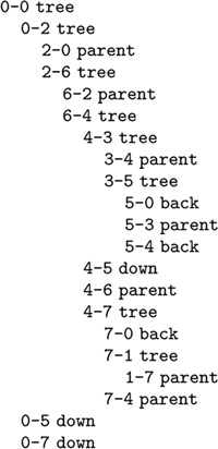
This version of Figure 18.5 shows the classification of the DFS tree link corresponding to each graph edge representation encountered. Tree edges (which correspond to recursive calls) are represented as tree links on the first encounter and parent links on the second encounter. Back edges are back links on the first encounter and down links on the second encounter.
The definitions just given provide sufficient information to distinguish among tree, parent, back, and down links in a DFS class implementation. Note that parent links and back links both have ord[w] < ord[v], so we have also to know that st[w] is not v to know that v-w is a back link. Figure 18.10 depicts the result of printing out the classification of the DFS tree link for each graph edge as that edge is encountered during a sample DFS. It is yet another complete representation of the basic search process that is an intermediate step between Figure 18.5 and Figure 18.9.
The four types of tree links correspond to the four different ways in which we treat edges during a DFS, as described (in maze-exploration terms) at the end of Section 18.1. A tree link corresponds to DFS encountering the first of the two representations of a tree edge, leading to a recursive call (to as-yet-unseen vertices); a parent link corresponds to DFS encountering the other representation of the tree edge (when going through the adjacency list on that first recursive call) and ignoring it. A back link corresponds to DFS encountering the first of the two representations of a back edge, which points to a vertex for which the recursive search function has not yet completed; a down link corresponds to DFS encountering a vertex for which the recursive search has completed at the time that the edge is encountered. In Figure 18.9, tree links and back links connect unshaded nodes, represent the first encounter with the corresponding edge, and constitute a representation of the graph; parent links and down links go to shaded nodes and represent the second encounter with the corresponding edge.
We have considered this tree representation of the dynamic characteristics of recursive DFS in detail not just because it provides a complete and compact description of both the graph and the operation of the algorithm, but also because it gives us a basis for understanding numerous important graph-processing algorithms. In the remainder of this chapter, and in the next several chapters, we consider a number of examples of graph-processing problems that draw conclusions about a graph’s structure from the DFS tree.
Search in a graph is a generalization of tree traversal. When invoked on a tree, DFS is precisely equivalent to recursive tree traversal; for graphs, using it corresponds to traversing a tree that spans the graph
Figure 18.11 DFS forest
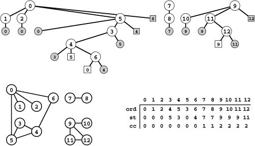
The DFS forest at the top represents a DFS of an adjacency-matrix representation of the graph at the bottom right. The graph has three connected components, so the forest has three trees. The ord vector is a preorder numbering of the nodes in the tree (the order in which they are examined by the DFS) and the st vector is a parent-link representation of the forest. The cc vector associates each vertex with a connected-component index (see Program 18.4). As in Figure 18.9, edges to circles are tree edges; edges that go to squares are back edges; and shaded nodes indicate that the incident edge was encountered earlier in the search, in the other direction.
and that is discovered as the search proceeds. As we have seen, the particular tree traversed depends on how the graph is represented. DFS corresponds to preorder tree traversal. In Section 18.6, we examine the graph-searching analog to level-order tree traversal and explore its relationship to DFS; in Section 18.7, we examine a general schema that encompasses any traversal method.
When traversing graphs with DFS, we have been using the ord vector to assign preorder numbers to the vertices in the order that we start processing them. We can also assign postorder numbers to vertices, in the order that we finish processing them (just before returning from the recursive search function). When processing a graph, we do more than simply traverse the vertices—as we shall see, the preorder and postorder numbering give us knowledge about global graph properties that helps us to accomplish the task at hand. Preorder numbering suffices for the algorithms that we consider in this chapter, but we use postorder numbering in later chapters.
We describe the dynamics of DFS for a general undirected graph with a DFS forest that has one DFS tree for each connected component. An example of a DFS forest is illustrated in Figure 18.11.
With an adjacency-lists representation, we visit the edges connected to each vertex in an order different from that for the adjacency-matrix representation, so we get a different DFS forest, as illustrated in Figure 18.12. DFS trees and forests are graph representations that describe not only the dynamics of DFS but also the internal representation
Figure 18.12 Another DFS forest
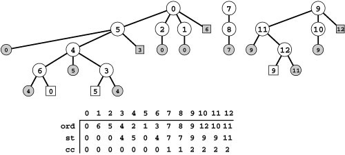
This forest describes depth-first search of the same graph as Figure 18.11, but using an adjacency-list representation, so the search order is different because it is determined by the order that nodes appear in adjacency lists. Indeed, the forest itself tells us that order: it is the order in which children are listed for each node in the tree. For instance, the nodes on 0’s adjacency list were found in the order 521 6, the nodes on 4’s list are in the order 653, and so forth. As before, all vertices and edges in the graph are examined during the search, in a manner that is precisely described by a preorder walk of the tree. The ord and st vectors depend upon the graph representation and the search dynamics and are different from Figure 18.11, but the vector cc depends on graph properties and is the same.
of the graph. For example, by reading the children of any node in Figure 18.12 from left to right, we see the order in which they appear on the adjacency list of the vertex corresponding to that node. We can have many different DFS forests for the same graph—each ordering of nodes on adjacency lists leads to a different forest.
Details of the structure of a particular forest inform our understanding of how DFS operates for particular graphs, but most of the important DFS properties that we consider depend on graph properties that are independent of the structure of the forest. For example, the forests in Figures 18.11 and 18.12 both have three trees (as would any other DFS forest for the same graph) because they are just different representations of the same graph, which has three connected components. Indeed, a direct consequence of the basic proof that DFS visits all the nodes and edges of a graph (see Properties 18.2 through 18.4) is that the number of connected components in the graph is equal to the number of trees in the DFS forest. This example illustrates the basis for our use of graph search throughout the book: A broad variety of graph-processing class implementations are based on learning graph properties by processing a particular graph representation (a forest corresponding to the search).
Potentially, we could analyze DFS tree structures with the goal of improving algorithm performance. For example, should we attempt to speed up an algorithm by rearranging the adjacency lists before starting the search? For many of the important classical DFS-based algorithms, the answer to this question is no, because they are optimal—their worst-case running time depends on neither the graph structure nor the order in which edges appear on the adjacency lists (they essentially process each edge exactly once). Still, DFS forests have a characteristic structure that is worth understanding because it distinguishes them from other fundamental search schema that we consider later in this chapter.
Figure 18.13 shows a DFS tree for a larger graph that illustrates the basic characteristics of DFS search dynamics. The tree is tall and thin, and it demonstrates several characteristics of the graph being searched and of the DFS process.
• There exists at least one long path that connects a substantial fraction of the nodes.
• During the search, most vertices have at least one adjacent vertex that we have not yet seen.
• We rarely make more than one recursive call from any node.
• The depth of the recursion is proportional to the number of vertices in the graph.
This behavior is typical for DFS, though these characteristics are not guaranteed for all graphs. Verifying facts of this kind for graph models of interest and various types of graphs that arise in practice requires detailed study. Still, this example gives an intuitive feel for DFS-based algorithms that is often borne out in practice. Figure 18.13 and similar figures for other graph-search algorithms (see Figures 18.24 and 18.29) help us understand differences in their behavior.
Exercises
18.15 Draw the DFS forest that results from a standard adjacency-matrix DFS of the graph
3-7 1-4 7-8 0-5 5-2 3-8 2-9 0-6 4-9 2-6 6-4.
18.16 Draw the DFS forest that results from a standard adjacency-lists DFS of the graph
3-7 1-4 7-8 0-5 5-2 3-8 2-9 0-6 4-9 2-6 6-4.
18.17 Write a DFS trace program to produce output that classifies each of the two representations of each graph edge as corresponding to a tree, parent, back, or down link in the DFS tree, in the style of Figure 18.10.
• 18.18 Write a program that computes a parent-link representation of the full DFS tree (including the external nodes), using an vector of E integers between 0 and V − 1. Hint: The first V entries in the vector should be the same as those in the st vector described in the text.
Figure 18.13 Depth-first search
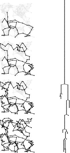
This figure illustrates the progress of DFS in a random Euclidean near-neighbor graph (left). The figures show the DFS tree vertices and edges in the graph as the search progresses through 1/4, 1/2, 3/4, and all of the vertices (top to bottom). The DFS tree (tree edges only) is shown at the right. As is evident from this example, the search tree for DFS tends to be quite tall and thin for this type of graph (as it is for many other types of graphs commonly encountered in practice). We normally find a vertex nearby that we have not seen before.
• 18.19 Instrument the spanning-forest DFS class (Program 18.3) by adding member functions (and appropriate private data members) that return the height of the tallest tree in the forest, the number of back edges, and the percentage of edges processed to see every vertex.
• 18.20 Run experiments to determine empirically the average values of the quantities described in Exercise 18.19 for graphs of various sizes, drawn from various graph models (see Exercises 17.64–76).
• 18.21 Write a function that builds a graph by inserting edges from a given vector into an initially empty graph, in random order. Using this function with an adjacency-lists implementation of the graph ADT, run experiments to determine empirically properties of the distribution of the quantities described in Exercise 18.19 for all the adjacency-lists representations of large sample graphs of various sizes, drawn from various graph models (see Exercises 17.64–76).
18.5 DFS Algorithms
Regardless of the graph structure or the representation, any DFS forest allows us to identify edges as tree or back edges and gives us dependable insights into graph structure that allow us to use DFS as a basis for solving numerous graph-processing problems. We have already seen, in Section 17.7, basic examples related to finding paths. In this section, we consider DFS-based ADT function implementations for these and other typical problems; in the remainder of this chapter and in the next several chapters, we look at numerous solutions to much more difficult problems.
Cycle detection Does a given graph have any cycles? (Is the graph a forest?) This problem is easy to solve with DFS because any back edge in a DFS tree belongs to a cycle consisting of the edge plus the tree path connecting the two nodes (see Figure 18.9). Thus, we can use DFS immediately to check for cycles: A graph is acyclic if and only if we encounter no back (or down!) edges during a DFS. For example, to test this condition in Program 18.1, we simply add an else clause to the if statement to test whether t is equal to v. If it is, we have just encountered the parent link w-v (the second representation of the edge v-w that led us to w). If it is not, w-t completes a cycle with the edges from t down to w in the DFS tree. Moreover, we do not need to examine all the edges: We know that we must find a cycle or finish the search without finding one before examining V edges, because any graph with V or more edges must have a cycle. Thus, we can test whether a graph is acyclic in time proportional to V with the adjacency-lists representation, although we may need time proportional to V2 (to find the edges) with the adjacency-matrix representation.
Simple path Given two vertices, is there a path in the graph that connects them? We saw in Section 17.7 that a DFS class that can solve this problem in linear time is easy to devise.
Simple connectivity As discussed in Section 18.3, we determine whether or not a graph is connected whenever we use DFS, in linear time. Indeed, our graph-search strategy is based upon calling a search function for each connected component. In a DFS, the graph is connected if and only if the graph-search function calls the recursive DFS function just once (see Program 18.2). The number of connected components in the graph is precisely the number of times that the recursive function is called from GRAPHsearch, so we can find the number of connected components by simply keeping track of the number of such calls.
More generally, Program 18.4 illustrates a DFS class that supports constant-time connectivity queries after a linear-time preprocessing step in the constructor. It visits vertices in the same order as does Program 18.3. The recursive function uses a vertex as its second argument instead of an edge, since it does not need to know the identity of the parent. Each tree in the DFS forest identifies a connected component, so we arrange to decide quickly whether two vertices are in the same component by including a vertex-indexed vector in the graph representation, to be filled in by a DFS and accessed for connectivity queries. In the recursive DFS function, we assign the current value of the component counter to the entry corresponding to each vertex visited. Then, we know that two vertices are in the same component if and only if their entries in this vector are equal. Again, note that this vector reflects structural properties of the graph, rather than artifacts of the graph representation or of the search dynamics.
Program 18.4 typifies the basic approach that we shall use in addressing numerous graph-processing tasks. We develop a task-specific class so that clients can create objects to perform the task. Typically, we invest preprocessing time in the constructor to compute private data about relevant structural graph properties that help us to provide efficient implementations of public query functions. In this case, the constructor
preprocesses with a (linear-time) DFS and keeps a private data member (the vertex-indexed vector id) that allows it to answer connectivity queries in constant time. For other graph-processing problems, our constructors might use more space, preprocessing time, or query time. As usual, our focus is on minimizing such costs, although doing so is often challenging. For example, much of Chapter 19 is devoted to solving the connectivity problem for digraphs, where achieving linear time preprocessing and constant query time, as in Program 18.4, is an elusive goal.
How does the DFS-based solution for graph connectivity in Program 18.4 compare with the union-find approach that we considered in Chapter 1 for the problem of determining whether a graph is connected, given an edge list? In theory, DFS is faster than union-find because it provides a constant-time guarantee, which union- find does not; in practice, this difference is negligible, and union-find is faster because it does not have to build a full representation of the graph. More important, union-find is an online algorithm (we can check whether two vertices are connected in near-constant time at any point), whereas the DFS solution preprocesses the graph to answer connectivity queries in constant time. Therefore, for example, we prefer union-find when determining connectivity is our only task or when we have a large number
Figure 18.14 A two-way Euler tour
Depth-first search gives us a way to explore any maze, traversing both passages in each direction. We modify Trémaux exploration to take the string with us wherever we go and take a back-and-forth trip on passages without any string in them that go to intersections that we have already visited. This figure shows a different traversal order than shown in Figures 18.2 and 18.3, primarily so that we can draw the tour without crossing itself. This ordering might result, for example, if the edges were processed in some different order when building an adjacency-lists representation of the graph; or, we might explicitly modify DFS to take the geometric placement of the nodes into account (see Exercise 18.26). Moving along the lower track leading out of 0, we move from 0 to 2 to 6 to 4 to 7, then take a trip from 7 to 0 and back because ord[0] is less than ord[7]. Then we go to 1, back to 7, back to 4, to 3, to 5, from 5 to 0 and back, from 5 to 4 and back, back to 3, back to 4, back to 6, back to 2, and back to 0. This path may be obtained by a recursive pre- and postorder walk of the DFS tree (ignoring the shaded vertices that represent the second time we encounter the edges) where we print out the vertex name, recursively visit the subtrees, then print out the vertex name again.
of queries intermixed with edge insertions but may find the DFS solution more appropriate for use in a graph ADT because it makes efficient use of existing infrastructure. Neither approach handles efficiently huge numbers of intermixed edge insertions, edge deletions, and connectivity queries; both require a separate DFS to compute the path. These considerations illustrate the complications that we face when analyzing graph algorithms; we explore them in detail in Section 18.9.
Two-way Euler tour Program 18.5 is a DFS-based class for finding a path that uses all the edges in a graph exactly twice—once in each direction (see Section 17.7). The path corresponds to a Trémaux exploration in which we take our string with us everywhere that we go, check for the string instead of using lights (so we have to go down the passages that lead to intersections that we have already visited), and first arrange to go back and forth on each back link (the first time that we encounter each back edge), then ignore down links (the second time that we encounter each back edge). We might also choose to ignore the back links (first encounter) and to go back and forth on down links (second encounter) (see Exercise 18.25).
Spanning forest Given a connected graph with V vertices, find a set of V − 1 edges that connects the vertices. If the graph has C connected components, find a spanning forest (with V - C edges). We have already seen a DFS class that solves this problem: Program 18.3.
Vertex search How many vertices are in the same connected component as a given vertex? We can solve this problem easily by starting a DFS at the vertex and counting the number of vertices marked. In a dense graph, we can speed up the process considerably by stopping the DFS after we have marked V vertices—at that point, we know that
Figure 18.15 Two-coloring a DFS tree
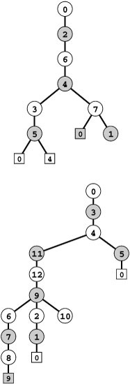
To two-color a graph, we alternate colors as we move down the DFS tree, then check the back edges for inconsistencies. In the tree at the top, a DFS tree for the sample graph illustrated in Figure 18.9, the back edges 5-4 and 7-0 prove that the graph is not two-colorable because of the odd-length cycles 4-3-5-4 and 0-2-6-4-7-0, respectively. In the tree at the bottom, a DFS tree for the bipartite graph illustrated in Figure 17.5, there are no such inconsistencies, and the indicated shading is a two-coloring of the graph.
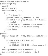
Program 18.6 Two-colorability (bipartiteness)
The constructor in this DFS class sets OK to true if and only if it is able to assign the values 0 or 1 to the vertex-indexed vector vc such that, for each graph edge v-w, vc[v] and vc[w] are different.
no edge will take us to a vertex that we have not yet seen, so we will be ignoring all the rest of the edges. This improvement is likely to allow us to visit all vertices in time proportional to V log V, not E (see Section 18.8).
Two-colorability, bipartiteness, odd cycle Is there a way to assign one of two colors to each vertex of a graph such that no edge connects two vertices of the same color? Is a given graph bipartite (see Section 17.1)? Does a given graph have a cycle of odd length? These three problems are all equivalent: The first two are different nomenclature for the same problem; any graph with an odd cycle is clearly not two-colorable, and Program 18.6 demonstrates that any graph that is free of odd cycles can be two-colored. The program is a DFS-based ADT function implementation that tests whether a graph is bipartite, two-colorable, and free of odd cycles. The recursive function is an outline for a proof by induction that the program two-colors any graph with no odd cycles (or finds an odd cycle as evidence that a graph that is not free of odd cycles cannot be two-colored). To two-color a graph with a given color assigned to a vertex v, two-color the remaining graph, assigning the other color to each vertex adjacent to v. This process is equivalent to assigning alternate colors on levels as we proceed down the DFS tree, checking back edges for consistency in the coloring, as illustrated in Figure 18.15. Any back edge connecting two vertices of the same color is evidence of an odd cycle.
These basic examples illustrate ways in which DFS can give us insight into the structure of a graph. They also demonstrate that we can learn various important graph properties in a single linear-time sweep through the graph, where we examine every edge twice, once in each direction. Next, we consider an example that shows the utility of DFS in discovering more intricate details about the graph structure, still in linear time.
Exercises
• 18.22 Implement a DFS-based cycle-testing class that preprocesses a graph in time proportional to V in the constructor to support public member functions for detecting whether a graph has any cycles and for printing a cycle if one exists.
18.23 Describe a family of graphs with V vertices for which a standard adjacency-matrix DFS requires time proportional to V2 for cycle detection.
• 18.24 Implement the graph-connectivity class of Program 18.4 as a derived graph-search class, like Program 18.3.
• 18.25 Specify a modification to Program 18.5 that will produce a two-way Euler tour that does the back-and-forth traversal on down edges instead of back edges.
• 18.26 Modify Program 18.5 such that it always produces a two-way Euler tour that, like the one in Figure 18.14, can be drawn such that it does not cross itself at any vertex. For example, if the search in Figure 18.14 were to take the edge 4-3 before the edge 4-7, then the tour would have to cross itself; your task is to ensure that the algorithm avoids such situations.
18.27 Develop a version of Program 18.5 that sorts the edges of a graph in order of a two-way Euler tour. Your program should return a vector of edges that corresponds to a two-way Euler tour.
18.28 Prove that a graph is two-colorable if and only if it contains no odd cycle. Hint: Prove by induction that Program 18.6 determines whether or not any given graph is two-colorable.
• 18.29 Explain why the approach taken in Program 18.6 does not generalize to give an efficient method for determining whether a graph is three-colorable.
18.30 Most graphs are not two-colorable, and DFS tends to discover that fact quickly. Run empirical tests to study the number of edges examined by Program 18.6, for graphs of various sizes, drawn from various graph models (see Exercises 17.64–76).
• 18.31 Prove that every connected graph has a vertex whose removal will not disconnect the graph, and write a DFS function that finds such a vertex. Hint: Consider the leaves of the DFS tree.
18.32 Prove that every graph with more than one vertex has at least two vertices whose removal will not increase the number of connected components.
18.6 Separability and Biconnectivity
To illustrate the power of DFS as the basis for graph-processing algorithms, we turn to problems related to generalized notions of connectivity in graphs. We study questions such as the following: Given two vertices, are there two different paths connecting them?
If it is important that a graph be connected in some situation, it might also be important that it stay connected when an edge or a vertex is removed. That is, we may want to have more than one route between each pair of vertices in a graph, so as to handle possible failures. For example, we can fly from New York to San Francisco even if Chicago is snowed in by going through Denver instead. Or, we might imagine a wartime situation where we want to arrange our railroad network such that an enemy must destroy at least two stations to cut our rail lines. Similarly, we might expect the main communications lines in an integrated circuit or a communications network to be connected such that the rest of the circuit still can function if one wire is broken or one link is down.
These examples illustrate two distinct concepts: In the circuit and in the communications network, we are interested in staying connected if an edge is removed; in the air or train routes, we are interested in staying connected if a vertex is removed. We begin by examining the former in detail.
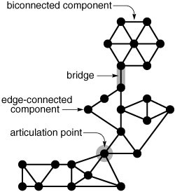
Figure 18.16 An edge-separable graph
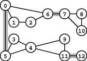
This graph is not edge connected. The edges 0-5, 6-7, and 11-12 (shaded) are separating edges (bridges). The graph has 4 edge-connected components: one comprising vertices 0, 1, 2, and 6; another comprising vertices 3, 4, 9, and 11; another comprising vertices 7, 8, and 10; and the single vertex 12.
Definition 18.1 A bridge in a graph is an edge that, if removed, would separate a connected graph into two disjoint subgraphs. A graph that has no bridges is said to be edge-connected.
When we speak of removing an edge, we mean to delete that edge from the set of edges that define the graph, even when that action might leave one or both of the edge’s vertices isolated. An edge-connected graph remains connected when we remove any single edge. In some contexts, it is more natural to emphasize our ability to disconnect the graph rather than the graph’s ability to stay connected, so we freely use alternate terminology that provides this emphasis: We refer to a graph that is not edge-connected as an edge-separable graph, and we call bridges separation edges. If we remove all the bridges in an edge-separable graph, we divide it into edge-connected components or bridge-connected components: maximal subgraphs with no bridges. Figure 18.16 is a small example that illustrates these concepts.
Finding the bridges in a graph seems, at first blush, to be a nontrivial graph-processing problem, but it actually is an application of DFS where we can exploit basic properties of the DFS tree that we have already noted. Specifically, back edges cannot be bridges because we know that the two nodes they connect are also connected by a path in the DFS tree. Moreover, we can add a simple test to our recursive DFS function to test whether or not tree edges are bridges. The basic idea, stated formally next, is illustrated in Figure 18.17.
Property 18.5 In any DFS tree, a tree edge v-w is a bridge if and only if there are no back edges that connect a descendant of w to an ancestor of w .
Proof: If there is such an edge, v-w cannot be a bridge. Conversely, if v-w is not a bridge, then there has to be some path from w to v in the graph other than w-v itself. Every such path has to have some such edge. •
Asserting this property is equivalent to saying that the only link in the subtree rooted at w that points to a node not in the subtree is the parent link from w back to v. This condition holds if and only if every path connecting any of the nodes in w’s subtree to any node that
Figure 18.17 DFS tree for finding bridges
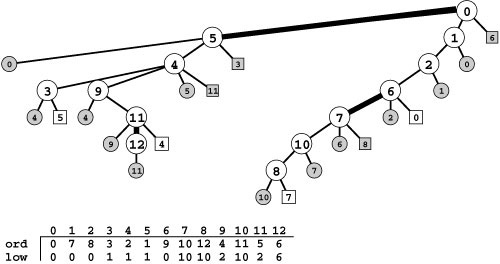
Nodes 5, 7, and 12 in this DFS tree for the graph in Figure 18.16 all have the property that no back edge connects a descendant with an ancestor, and no other nodes have that property. Therefore, as indicated, breaking the edge between one of these nodes and its parent would disconnect the subtree rooted at that node from the rest of the graph. That is, the edges 0-5, 11-12, and 6-7 are bridges. We use the vertex-indexed array low to keep track of the lowest preorder number (ord value) referenced by any back edge in the subtree rooted at the vertex. For example, the value of low[9] is 2 because one of the back edges in the subtree rooted at 9 points to 4 (the vertex with preorder number 2), and no other back edge points higher in the tree. Nodes 5, 7, and 12 are the ones for which the low value is equal to the ord value.
is not in w’s subtree includes v-w. In other words, removing v-w would disconnect from the rest of the graph the subgraph corresponding to w’s subtree.
Program 18.7 shows how we can augment DFS to identify bridges in a graph, using Property 18.5. For every vertex v, we use the recursive function to compute the lowest preorder number that can be reached by a sequence of zero or more tree edges followed by a single back edge from any node in the subtree rooted at v. If the computed number is equal to v’s preorder number, then there is no edge connecting a descendant with an ancestor, and we have identified a bridge. The computation for each vertex is straightforward: We proceed through the adjacency list, keeping track of the minimum of the numbers that we can reach by following each edge. For tree edges, we do the computation recursively; for back edges, we use the preorder number of the adjacent vertex. If the call to the recursive function for an edge w-t does not uncover a path to a node with a preorder number less than t’s preorder number, then w-t is a bridge.
Property 18.6 We can find a graph’s bridges in linear time.
Proof: Program 18.7 is a minor modification to DFS that involves adding a few constant-time tests, so it follows directly from Properties 18.3 and 18.4 that finding the bridges in a graph requires time proportional to V2 for the adjacency-matrix representation and to V + E for the adjacency-lists representation.•
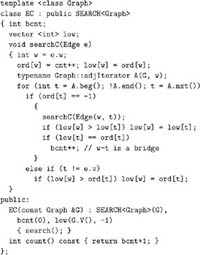
Program 18.7 Edge connectivity
This DFS class counts the bridges in a graph. Clients can use an EC object to find the number of edge-connected components; adding a member function for testing whether two vertices are in the same edge-connected component is left as an exercise (see Exercise 18.36). The low vector keeps track of the lowest preorder number that can be reached from each vertex by a sequence of tree edges followed by one back edge.
In Program 18.7, we use DFS to discover properties of the graph. The graph representation certainly affects the order of the search, but it does not affect the results because bridges are a characteristic of the graph rather than of the way that we choose to represent or search
Figure 18.18 Another DFS tree for finding bridges
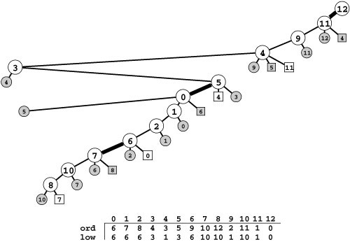
This diagram shows a different DFS tree than the one in Figure 18.17 for the graph in Figure 18.16, where we start the search at a different node. Although we visit the nodes and edges in a completely different order, we still find the same bridges (of course). In this tree, 0, 7, and 11 are the ones for which the low value is equal to the ord value, so the edges connecting each of them to their parents (12-11, 5-0, and 6-7, respectively) are bridges.
the graph. As usual, any DFS tree is simply another representation of the graph, so all DFS trees have the same connectivity properties. The correctness of the algorithm depends on this fundamental fact. For example, Figure 18.18 illustrates a different search of the graph, starting from a different vertex, that (of course) finds the same bridges. Despite Property 18.6, when we examine different DFS trees for the same graph, we see that some search costs may depend not just on properties of the graph but also on properties of the DFS tree. For example, the amount of space needed for the stack to support the recursive calls is larger for the example in Figure 18.18 than for the example in Figure 18.17.
As we did for regular connectivity in Program 18.4, wemaywish to use Program 18.7 to build a class for testing whether a graph is edge-connected or to count the number of edge-connected components. If desired, we can proceed as for Program 18.4 to gives clients the ability to create (in linear time) objects that can respond in constant time to queries that ask whether two vertices are in the same edge-connected component (see Exercise 18.36).
We conclude this section by considering other generalizations of connectivity, including the problem of determining which vertices are critical to keeping a graph connected. By including this material here, we keep in one place the basic background material for the more complex algorithms that we consider in Chapter 22. If you are new to connectivity problems, you may wish to skip to Section 18.7 and return here when you study Chapter 22.
When we speak of removing a vertex, we also mean that we remove all its incident edges. As illustrated in Figure 18.19, removing either of the vertices on a bridge would disconnect a graph (unless the bridge were the only edge incident on one or both of the vertices), but there are also other vertices, not associated with bridges, that have the same property.
Definition 18.2 An articulation point in a graph is a vertex that, if removed, would separate a connected graph into at least two disjoint subgraphs.
We also refer to articulation points as separation vertices or cut vertices. We might use the term “vertex connected” to describe a graph that has no separation vertices, but we use different terminology based on a related characterization that turns out to be equivalent.
Definition 18.3 A graph is said to be biconnected if every pair of vertices is connected by two disjoint paths.
The requirement that the paths be disjoint is what distinguishes biconnectivity from edge connectivity. An alternate definition of edge connectivity is that every pair of vertices is connected by two edge-disjoint paths—these paths can have a vertex (but no edge) in common. Biconnectivity is a stronger condition: An edge-connected graph remains connected if we remove any edge, but a biconnected graph remains connected if we remove any vertex (and all that vertex’s incident edges). Every biconnected graph is edge-connected, but an edge-connected graph need not be biconnected. We also use the term separable to refer to graphs that are not biconnected, because they can be separated into two pieces by removal of just one vertex. The separation vertices are the key to biconnectivity.
Property 18.7 A graph is biconnected if and only if it has no separation vertices (articulation points).
Proof: Assume that a graph has a separation vertex. Let s and t be vertices that would be in two different pieces if the separation vertex were removed. All paths between s and t must contain the separation vertex, therefore the graph is not biconnected. The proof in the other direction is more difficult and is a worthwhile exercise for the mathematically inclined reader (see Exercise 18.40).•
Figure 18.19 Graph separability terminology
This graph has two edge-connected components and one bridge. The edge-connected component above the bridge is also biconnected; the one below the bridge consists of two biconnected components that are joined at an articulation point.
Figure 18.20 Articulation points (separation vertices)
This graph is not biconnected. The vertices 0, 4, 5, 6, 7, and 11 (shaded) are articulation points. The graph has five biconnected components: one comprising edges 4-9, 9-11, and 4-11; another comprising edges 7-8, 8-10, and 7-10; another comprising edges 0-1, 1-2, 2-6, and 6-0; another comprising edges 3-5, 4-5, and 3-4; and the single vertex 12. Adding an edge connecting 12 to 7, 8, or 10 would biconnect the graph.
We have seen that we can partition the edges of a graph that is not connected into a set of connected subgraphs, and that we can partition the edges of a graph that is not edge-connected into a set of bridges and edge-connected subgraphs (which are connected by bridges). Similarly, we can divide any graph that is not biconnected into a set of bridges and biconnected components, which are each biconnected subgraphs. The biconnected components and bridges are not a proper partition of the graph because articulation points may appear on multiple biconnected components (see, for example, Figure 18.20). The biconnected components are connected at articulation points, perhaps by bridges.
A connected component of a graph has the property that there exists a path between any two vertices in the graph. Analogously, a biconnected component has the property that there exist two disjoint paths between any pair of vertices.
We can use the same DFS-based approach that we used in Program 18.7 to determine whether or not a graph is biconnected and to identify the articulation points. We omit the code because it is very similar to Program 18.7, with an extra test to check whether the root of the DFS tree is an articulation point (see Exercise 18.43). Developing code to print out the biconnected components is also a worthwhile exercise that is only slightly more difficult than the corresponding code for edge connectivity (see Exercise 18.44).
Property 18.8 We can find a graph’s articulation points and biconnected components in linear time.
Proof: As for Property 18.7, this fact follows from the observation that the solutions to Exercises 18.43 and 18.44 involve minor modifications to DFS that amount to adding a few constant-time tests per edge.
Biconnectivity generalizes simple connectivity. Further generalizations have been the subjects of extensive studies in classical graph theory and in the design of graph algorithms. These generalizations indicate the scope of graph-processing problems that we might face, many of which are easily posed but less easily solved.
Definition 18.4 Agraphis k-connected if there are at least k vertex-disjoint paths connecting every pair of vertices in the graph. The vertex connectivity of a graph is the minimum number of vertices that need to be removed to separate it into two pieces.
In this terminology, “1-connected” is the same as “connected” and “2-connected” is the same as “biconnected.” A graph with an articulation point has vertex connectivity 1 (or 0), so Property 18.7 says that a graph is 2-connected if and only if its vertex connectivity is not less than 2. It is a special case of a classical result from graph theory, known as Whitney’s theorem, which says that a graph is k -connected if and only if its vertex connectivity is not less than k. Whitney’s theorem follows directly from Menger’s theorem (see Section 22.7), which says that the minimum number of vertices whose removal disconnects two vertices in a graph is equal to the maximum number of vertex-disjoint paths between the two vertices (to prove Whitney’s theorem, apply Menger’s theorem to every pair of vertices).
Definition 18.5 A graph is k–edge-connected if there are at least k edge-disjoint paths connecting every pair of vertices in the graph. The edge connectivity of a graph is the minimum number of edges that need to be removed to separate it into two pieces.
In this terminology, “2–edge-connected” is the same as “edge-connected” (that is, an edge-connected graph has edge connectivity greater than 1, and a graph with at least one bridge has edge connectivity 1). Another version of Menger’s theorem says that the minimum number of vertices whose removal disconnects two vertices in a graph is equal to the maximum number of vertex-disjoint paths between the two vertices, which implies that a graph is k –edge-connected if and only if its edge connectivity is k.
With these definitions, we are led to generalize the connectivity problems that we considered at the beginning of this section.
st-connectivity What is the minimum number of edges whose removal will separate two given vertices s and t in a given graph? What is the minimum number of vertices whose removal will separate two given vertices s and t in a given graph?
General connectivity Is a given graph k -connected? Is a given graph k –edge-connected? What is the edge connectivity and the vertex connectivity of a given graph?
Although these problems are much more difficult to solve than are the simple connectivity problems that we have considered in this section, they are members of a large class of graph-processing problems that we can solve using the general algorithmic tools that we consider in Chapter 22 (with DFS playing an important role); we consider specific solutions in Section 22.7.
Exercises
• 18.33 If a graph is a forest, all its edges are separation edges; but which vertices are separation vertices?
• 18.34 Consider the graph
3-7 1-4 7-8 0-5 5-2 3-8 2-9 0-6 4-9 2-6 6-4.
Draw the standard adjacency-lists DFS tree. Use it to find the bridges and the edge-connected components.
18.35 Prove that every vertex in any graph belongs to exactly one edge-connected component.
• 18.36 Add a public member function to Program 18.7 that allows clients to test whether two vertices are in the same edge-connected component.
• 18.37 Consider the graph
3-7 1-4 7-8 0-5 5-2 3-8 2-9 0-6 4-9 2-6 6-4.
Draw the standard adjacency-lists DFS tree. Use it to find the articulation points and the biconnected components.
• 18.38 Do the previous exercise using the standard adjacency-matrix DFS tree.
18.39 Prove that every edge in a graph either is a bridge or belongs to exactly one biconnected component.
• 18.40 Prove that any graph with no articulation points is biconnected. Hint: Given a pair of vertices s and t and a path connecting them, use the fact that none of the vertices on the path are articulation points to construct two disjoint paths connecting s and t.
18.41 Derive a class from Program 18.2 for determining whether a graph is biconnected, using a brute-force algorithm that runs in time proportional to V (V + E ). Hint: If you mark a vertex as having been seen before you start the search, you effectively remove it from the graph.
• 18.42 Extend your solution to Exercise 18.41 to derive a class that determines whether a graph is 3-connected. Give a formula describing the approximate number of times your program examines a graph edge, as a function of V and E.
18.43 Prove that the root of a DFS tree is an articulation point if and only if it has two or more (internal) children.
• 18.44 Derive a class from Program 18.2 that prints the biconnected components of the graph.
18.45 What is the minimum number of edges that must be present in any biconnected graph with V vertices?
18.46 Modify Program 18.7 to simply determine whether or not the graph is edge-connected (returning as soon as it identifies a bridge if the graph is not) and instrument it to keep track of the number of edges examined. Run empirical tests to study this cost, for graphs of various sizes, drawn from various graph models (see Exercises 17.64–76).
• 18.47 Derive a class from Program 18.2 that allows clients to create objects that know the number of articulation points, bridges, and biconnected components in a graph.
• 18.48 Run experiments to determine empirically the average values of the quantities described in Exercise 18.47 for graphs of various sizes, drawn from various graph models (see Exercises 17.64–76).
18.49 Give the edge connectivity and the vertex connectivity of the graph
0-1 0-2 0-8 2-1 2-8 8-1 3-8 3-7 3-6 3-5 3-4 4-6 4-5 5-6 6-7 7-8.
18.7 Breadth-First Search
Suppose that we want to find a shortest path between two specific vertices in a graph—a path connecting the vertices with the property that no other path connecting those vertices has fewer edges. The classical method for accomplishing this task, called breadth-first search (BFS), is also the basis of numerous algorithms for processing graphs, so we consider it in detail in this section. DFS offers us little assistance in solving this problem, because the order in which it takes us through the graph has no relationship to the goal of finding shortest paths. In contrast, BFS is based on this goal. To find a shortest path from v to w, we start at v and check for w among all the vertices that we can reach by following one edge, then we check all the vertices that we can reach by following two edges, and so forth.
When we come to a point during a graph search where we have more than one edge to traverse, we choose one and save the others to be explored later. In DFS, we use a pushdown stack (that is managed by the system to support the recursive search function) for this purpose. Using the LIFO rule that characterizes the pushdown stack corresponds to exploring passages that are close by in a maze: We
Figure 18.21 Breadth-first search
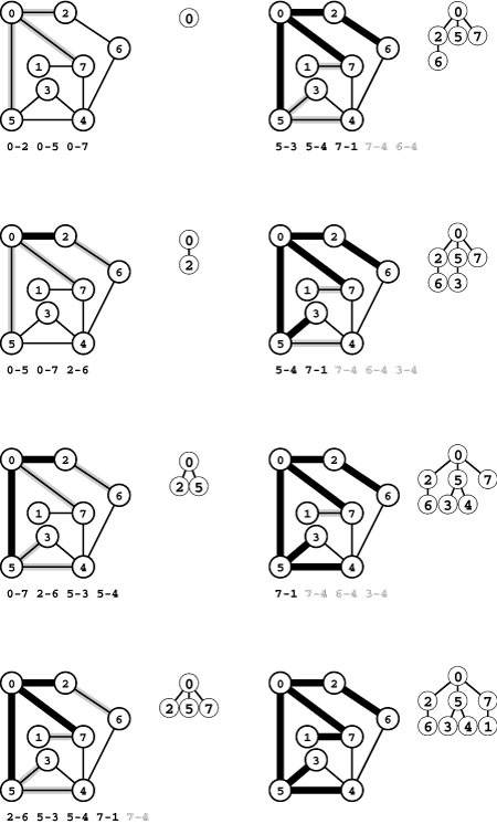
This figure traces the operation of BFS on our sample graph. We begin with all the edges adjacent to the start vertex on the queue (top left). Next, we move edge 0-2 from the queue to the tree and process its incident edges 2-0 and 2-6 (second from top, left). We do not put 2-0 on the queue because 0 is already on the tree. Third, we move edge 0-5 from the queue to the tree; again 5’s incident edge (to 0) leads nowhere new, but we add 5-3 and 5-4 to the queue (third from top, left). Next, we add 0-7 to the tree and put 7-1 on the queue (bottom left).
The edge 7-4 is printed in gray because we could also avoid putting it on the queue, since there is another edge that will take us to 4 that is already on the queue. To complete the search, we take the remaining edges off the queue, completely ignoring the gray edges when they come to the front of the queue (right). Edges enter and leave the queue in order of their distance from 0.
choose, of the passages yet to be explored, the one that was most recently encountered. In BFS, we want to explore the vertices in order of their distance from the start. For a maze, doing the search in this order might require a search team; within a computer program, however, it is easily arranged: We simply use a FIFO queue instead of a stack.
Program 18.8 is an implementation of BFS. It is based on maintaining a queue of all edges that connect a visited vertex with an unvisited vertex. We put a dummy self-loop to the start vertex on the queue, then perform the following steps until the queue is empty:
• Take edges from the queue until finding one that points to an unvisited vertex.
• Visit that vertex; put onto the queue all edges that go from that vertex to unvisited vertices.
Figure 18.21 shows the step-by-step development of BFS on a sample graph.
As we saw in Section 18.4, DFS is analogous to one person exploring a maze. BFS is analogous to a group of people exploring by fanning out in all directions. Although DFS and BFS are different in many respects, there is an essential underlying relationship between the two methods—one that we noted when we briefly considered the methods in Chapter 5. In Section 18.8, we consider a generalized graph-searching method that we can specialize to include these two algorithms and a host of others. Each algorithm has particular dynamic characteristics that we use to solve associated graph-processing problems. For BFS, the distance from each vertex to the start vertex (the length of a shortest path connecting the two) is the key property of interest.
Property 18.9 During BFS, vertices enter and leave the FIFO queue in order of their distance from the start vertex.
Proof: A stronger property holds: The queue always consists of zero or more vertices of distance k from the start, followed by zero or more vertices of distance k + 1 from the start, for some integer k. This stronger property is easy to prove by induction.
For DFS, we understood the dynamic characteristics of the algorithm with the aid of the DFS search forest that describes the recursive-call structure of the algorithm. An essential property of that forest is that the forest represents the paths from each vertex back to the place
Program 18.8 Breadth-first search
This graph-search class visits a vertex by scanning through its incident edges, putting any edges to unvisited vertices onto the queue of vertices to be visited. Vertices are marked in the visit order given by the vector ord. The search function that is called by the constructor builds an explicit parent-link representation of the BFS tree (the edges that first take us to each node) in another vector st, which can be used to solve basic shortest-paths problems (see text).
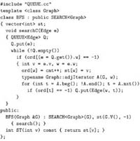
that the search started for its connected component. As indicated in the implementation and shown in Figure 18.22, such a spanning tree also helps us to understand BFS. As with DFS, we have a forest that characterizes the dynamics of the search, one tree for each connected component, one tree node for each graph vertex, and one tree edge for each graph edge. BFS corresponds to traversing each of the trees in this forest in level order. As with DFS, we use a vertex-indexed vector
to represent explicitly the forest with parent links. For BFS, this forest carries essential information about the graph structure:
Property 18.10 For any node w in the BFS tree rooted at v, the tree path from v to w corresponds to a shortest path from v to w in the corresponding graph.
Proof: The tree-path lengths from nodes coming off the queue to the root are nondecreasing, and all nodes closer to the root than w are on the queue; so no shorter path to w was found before it comes off the queue, and no path to w that is discovered after it comes off the queue can be shorter than w’s tree path length. •
As indicated in Figure 18.21 and noted in Chapter 5, there is no need to put an edge on the queue with the same destination vertex as any edge already on the queue, since the FIFO policy ensures that we will process the old queue edge (and visit the vertex) before we get to the new edge. One way to implement this policy is to use a queue ADT implementation where such duplication is disallowed by an ignore-the-new-item policy (see Section 4.7). Another choice is to use the global vertex-marking vector for this purpose: Instead of marking a vertex as having been visited when we take it off the queue,
Figure 18.22 BFS tree
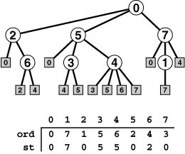
This tree provides a compact description of the dynamic properties of BFS, in a manner similar to the tree depicted in Figure 18.9. Traversing the tree in level order tells us how the search proceeds, step by step: first we visit 0; then we visit 2, 5, and 7; then we check from 2 that 0 was visited and visit 6; and so forth. Each tree node has a child representing each of the nodes adjacent to it, in the order they were considered by the BFS. As in Figure 18.9, links in the BFS tree correspond to edges in the graph: if we replace edges to external nodes by lines to the indicated node, we have a drawing of the graph. Links to external nodes represent edges that were not put onto the queue because they led to marked nodes: they are either parent links or cross links that point to a node either on the same level or one level closer to the root.
The st vector is a parent-link representation of the tree, which we can use to find a shortest path from any node to the root. For example, 3-5-0 is a path in the graph from 3 to 0, since st[3] is 5 and st[5] is 0. No other path from 3 to 0 is shorter.
we do so when we put it on the queue. Testing whether a vertex is marked (whether its entry has changed from its initial sentinel value) then stops us from putting any other edges that point to the same vertex on the queue. This change, shown in Program 18.9, gives a BFS implementation where there are never more than V edges on the queue (one edge pointing to each vertex, at most).
Property 18.11 BFS visits all the vertices and edges in a graph in time proportional to V2for the adjacency-matrix representation and to V + E for the adjacency-lists representation.
Proof: As we did in proving the analogous DFS properties, we note by inspecting the code that we check each entry in the adjacency-matrix row or in the adjacency list precisely once for every vertex that we visit, so it suffices to show that we visit each vertex. Now, for each connected component, the algorithm preserves the following invariant: All vertices that can be reached from the start vertex (i) are on the BFS tree, (ii) are on the queue, or (iii) can be reached from a vertex on the queue. Each vertex moves from (iii) to (ii) to (i), and the number of vertices in (i) increases on each iteration of the loop, so that the BFS tree eventually contains all the vertices that can be reached from the start vertex. Thus, as we did for DFS, we consider BFS to be a linear-time algorithm.
With BFS, we can solve the spanning tree, connected components, vertex search, and several other basic connectivity problems that we described in Section 18.4, since the solutions that we considered depend on only the ability of the search to examine every node and edge connected to the starting point. As we shall see, BFS and DFS are representative of numerouus algorithms that have this property. Our primary interest in BFS, as mentioned at the outset of this section, is that it is the natural graph-search algorithm for applications where we want to know a shortest path between two specified vertices. Next, we consider a specific solution to this problem and its extension to solve two related problems.
Shortest path Find a shortest path in the graph from v to w. We can accomplish this task by starting a BFS that maintains the parent-link representation st of the search tree at v, then stopping when we reach w. The path up the tree from w to v is a shortest path. For example, after construction a BFS<Graph> object bfs a client could use the following code to print the path connecting w to v:
for (t = w; t !=v; t = bfs.ST(t)) cout << t << “-”;
cout << v << endl;
To get the path from v to w, replace the cout operations in this code by stack pushes, then go into a loop that prints the vertex indices after popping them from the stack. Or, start the search at w and stop at v in the first place.
Single-source shortest paths Find shortest paths connecting a given vertex v with each other vertex in the graph. The full BFS tree rooted at v provides a way to accomplish this task: The path from each vertex to the root is a shortest path to the root. Therefore, to solve the problem, we run BFS to completion starting at v. The st vector that results from this computation is a parent-link representation of the BFS tree, and the code in the previous paragraph will give the shortest path to any other vertex w.
All-pairs shortest paths Find shortest paths connecting each pair of vertices in the graph. The way to accomplish this task is to use a BFS class that solves the single-source problem for each vertex in the graph and supports member functions that can handle huge numbers of shortest-path queries efficiently by storing the path lengths and parent-link tree representations for each vertex (see Figure 18.23). This preprocessing requires time proportional to V E and space proportional to V2, a potentially prohibitive cost for huge sparse graphs. However, it allows us to build an ADT with optimal performance: After investing in the preprocessing (and the space to hold the results), we can return shortest-path lengths in constant time and the paths themselves in time proportional to their length (see Exercise 18.55).
These BFS-based solutions are effective, but we do not consider implementations in any further detail here, because they are special cases of algorithms that we consider in detail in Chapter 21. The term shortest paths in graphs is generally taken to describe the corresponding problems for digraphs and networks. Chapter 21 is devoted to this topic. The solutions that we examine there are strict generalizations of the BFS-based solutions described here.
The basic characteristics of BFS search dynamics contrast sharply with those for DFS search, as illustrated in the large graph depicted in Figure 18.24, which you should compare with Figure 18.13. The tree
Figure 18.23 All-pairs shortest paths example
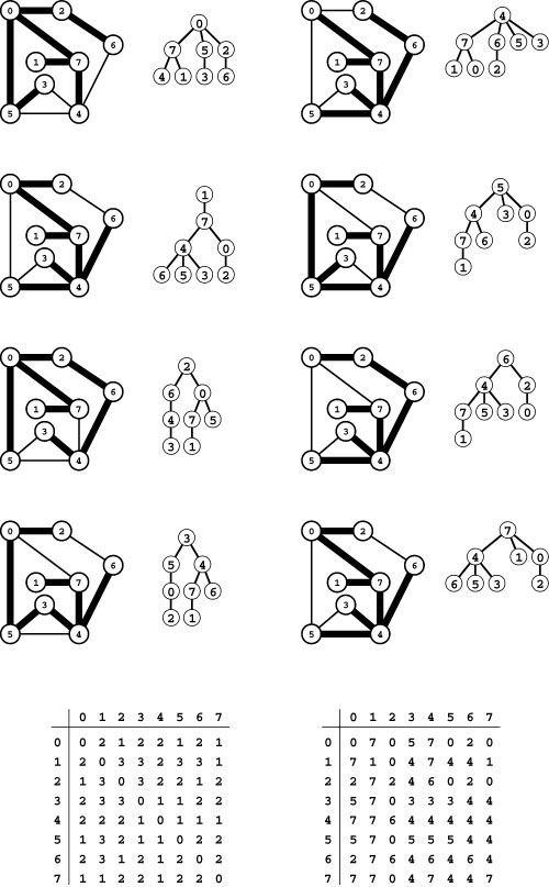
These figures depict the result of doing BFS from each vertex, thus computing the shortest paths connecting all pairs of vertices. Each search gives a BFS tree that defines the shortest paths connecting all graph vertices to the vertex at the root. The results of all the searches are summarized in the two matrices at the bottom. In the left matrix, the entry in row v and column w gives the length of the shortest path from v to w (the depth of v in w’s tree). Each row of the right matrix contains the st array for the corresponding search. For example, the shortest path from 3 to 2 has three edges, as indicated by the entry in row 3 and column 2 of the left matrix. The third BFS tree from the top on the left tells us that the path is 3-4-6-2, and this information is encoded in row 2 in the right matrix. The matrix is not necessarily symmetric when there is more than one shortest path, because the paths found depend on the BFS search order. For example, the BFS tree at the bottom on the left and row 3 of the right matrix tell us that the shortest path from 2 to 3 is 2-0-5-3.
Figure 18.24 Breadth-first search
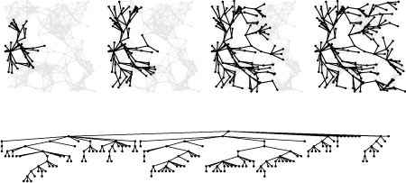
This figure illustrates the progress of BFS in random Euclidean near-neighbor graph (left), in the same style as Figure 18.13. As is evident from this example, the search tree for BFS tends to be quite short and wide for this type of graph (and many other types of graphs commonly encountered in practice). That is, vertices tend to be connected to one another by rather short paths. The contrast between the shapes of the DFS and BFS trees is striking testimony to the differing dynamic properties of the algorithms.
is shallow and broad, and demonstrates a set of facts about the graph being searched different from those shown by DFS. For example,
• There exists a relatively short path connecting each pair of vertices in the graph.
• During the search, most vertices are adjacent to numerous unvisited vertices.
Again, this example is typical of the behavior that we expect from BFS, but verifying facts of this kind for graph models of interest and graphs that arise in practice requires detailed analysis.
DFS wends its way through the graph, storing on the stack the points where other paths branch off; BFS sweeps through the graph, using a queue to remember the frontier of visited places. DFS explores the graph by looking for new vertices far away from the start point, taking closer vertices only when dead ends are encountered; BFS completely covers the area close to the starting point, moving farther away only when everything nearby has been examined. The order in which the vertices are visited depends on the graph structure and representation, but these global properties of the search trees are more informed by the algorithms than by the graphs or their representations.
The key to understanding graph-processing algorithms is to realize not only that various different search strategies are effective ways to learn various different graph properties, but also that we can implement many of them uniformly. For example, the DFS illustrated in Figure 18.13 tells us that the graph has a long path, and the BFS illustrated in Figure 18.24 tells us that it has many short paths. Despite these marked dynamic differences, DFS and BFS are similar, essentially differing in only the data structure that we use to save edges that are not yet explored (and the fortuitous circumstance that we can use a recursive implementation for DFS with the system maintaining an implicit stack for us). Indeed, we turn next to a generalized graph-search algorithm that encompasses DFS, BFS, and a host of other useful strategies and will serve as the basis for solutions to numerous classic graph-processing problems.
Exercises
18.50 Draw the BFS forest that results from a standard adjacency-lists BFS of the graph
3-7 1-4 7-8 0-5 5-2 3-8 2-9 0-6 4-9 2-6 6-4.
18.51 Draw the BFS forest that results from a standard adjacency-matrix BFS of the graph
3-7 1-4 7-8 0-5 5-2 3-8 2-9 0-6 4-9 2-6 6-4.
• 18.52 Modify Programs 18.8 and 18.9 to use an STL queue instead of the ADT from Section 4.8.
• 18.53 Give a BFS implementation (a version of Program 18.9) that uses a queue of vertices (see Program 5.22). Include a test in the BFS search code to ensure that no duplicates go on the queue.
18.54 Give the all-shortest-path matrices (in the style of Figure 18.23) for the graph
3-7 1-4 7-8 0-5 5-2 3-8 2-9 0-6 4-9 2-6 6-4,
assuming that you use the adjacency-matrix representation.
18.55 Develop a shortest-paths class, which supports shortest-path queries after preprocessing to compute all shortest paths. Specifically, define a two-dimensional matrix as a private data member, and write a constructor that assigns values to all its entries as illustrated in Figure 18.23. Then, implement two query functions length(v, w) (that returns the shortest-path length between v and w) and path(v, w) (that returns the vertex adjacent to v that is on a shortest path between v and w).
• 18.56 What does the BFS tree tell us about the distance from v to w when neither is at the root?
18.57 Develop a class whose objects know the path length that suffices to connect any pair of vertices in a graph. (This quantity is known as the graph’s diameter). Note: You need to define a convention for the return value in the case that the graph is not connected.
18.58 Give a simple optimal recursive algorithm for finding the diameter of a tree (see Exercise 18.57).
• 18.59 Instrument the BFS class Program 18.9 by adding member functions (and appropriate private data members) that return the the height of the BFS tree and the percentage of edges that must be processed for every vertex to be seen.
• 18.60 Run experiments to determine empirically the average values of the quantities described in Exercise 18.59 for graphs of various sizes, drawn from various graph models (see Exercises 17.64–76).
18.8 Generalized Graph Search
DFS and BFS are fundamental and essential graph-traversal methods that lie at the heart of numerous graph-processing algorithms. Knowing their essential properties, we now move to a higher level of abstraction, where we see that both methods are special cases of a generalized strategy for moving through a graph, one that is suggested by our BFS implementation (Program 18.9).
The basic idea is simple: We revisit our description of BFS from Section 18.6, but we use the term generic term fringe, instead of queue, to describe the set of edges that are possible candidates for being next added to the tree. We are led immediately to a general strategy for searching a connected component of a graph. Starting with a self-loop to a start vertex on the fringe and an empty tree, perform the following operation until the fringe is empty:
Move an edge from the fringe to the tree. If the vertex to which it leads is unvisited, visit that vertex, and put onto the fringe all edges that lead from that vertex to unvisited vertices.
This strategy describes a family of search algorithms that will visit all the vertices and edges of a connected graph,no matter what type of generalized queue we use to hold the fringe edges.
When we use a queue to implement the fringe, we get BFS, the topic of Section 18.6. When we use a stack to implement the fringe, we get DFS. Figure 18.25, which you should compare with Figures 18.6
Figure 18.25 Stack-based DFS
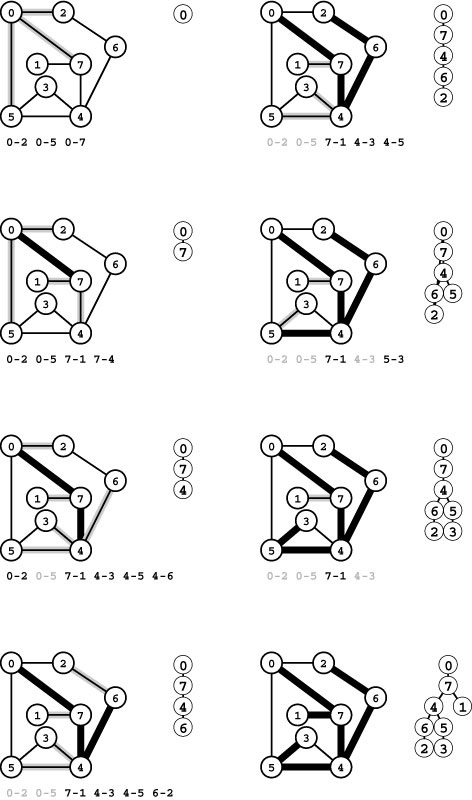
Together with Figure 18.21, this figure illustrates that BFS and DFS differ only in the underlying data structure. For BFS, we used a queue; for DFS we use a stack. We begin with all the edges adjacent to the start vertex on the stack (top left). Second, we move edge 0-7 from the stack to the tree and push onto the stack its incident edges that go to vertices not yet on the tree 7-1, 7-4, and 7-6 (second from top, left). The LIFO stack discipline implies that, when we put an edge on the stack, any edges that point to the same vertex are obsolete and will be ignored when they reach the top of the stack. Such edges are printed in gray. Third, we move edge 7-6 from the stack to the tree and push its incident edges on the stack (third from top, left). Next, we pop edge 4-6 and push its incident edges on the stack, two of which will take us to new vertices (bottom left). To complete the search, we take the remaining edges off the stack, completely ignoring the gray edges when they come to the top of the stack (right).
and 18.21, illustrates this phenomenon in detail. Proving this equivalence between recursive and stack-based DFS is an interesting exercise in recursion removal, where we essentially transform the stack underlying the recursive program into the stack implementing the fringe (see Exercise 18.63). The search order for the DFS depicted in Figure 18.25 differs from the one depicted in Figure 18.6 only because the stack discipline implies that we check the edges incident on each vertex in reverse of the order that we encounter them in the adjacency matrix (or the adjacency lists). The basic fact remains that, if we change the data structure used by Program 18.8 to be a stack instead of a queue (which is trivial to do because the ADT interfaces of the two data structures differ in only the function names), then we change that program from BFS to DFS.
Now, as we discussed in Section 18.7, this general method may not be as efficient as we would like, because the fringe becomes cluttered up with edges that point to vertices that are moved to the tree during the time that the edge is on the fringe. For FIFO queues, we avoid this situation by marking destination vertices when we put edges on the queue. We ignore edges to fringe vertices because we know that they will never be used: The old one will come off the queue (and the vertex visited) before the new one does (see Program 18.9). For a stack implementation, we want the opposite: When an edge is to be added to the fringe that has the same destination vertex as the one already there, we know that the old edge will never be used, because the new one will come off the stack (and the vertex visited) before the old one. To encompass these two extremes and to allow for fringe implementations that can use some other policy to disallow edges on the fringe that point to the same vertex, we modify our general scheme as follows:
Move an edge from the fringe to the tree. Visit the vertex that it leads to, and put all edges that lead from that vertex to unvisited vertices onto the fringe, using a replacement policy on the fringe that ensures that no two edges on the fringe point to the same vertex.
The no-duplicate-destination-vertex policy on the fringe guarantees that we do not need to test whether the destination vertex of the edge coming off the queue has been visited. For BFS, we use a queue implementation with an ignore-the-new-item policy; for DFS, we need
Figure 18.26 Graph search terminology

During a graph search, we maintain a search tree (black) and a fringe (gray) of edges that are candidates to be next added to the tree. Each vertex is either on the tree (black), the fringe (gray), or not yet seen (white). Tree vertices are connected by tree edges, and each fringe vertex is connected by a fringe edge to a tree vertex.
Figure 18.27 Graph search strategies
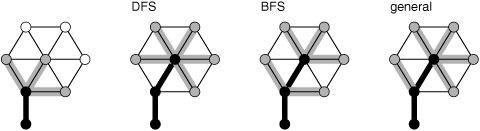
This figure illustrates different possibilities when we take a next step in the search illustrated in Figure 18.26. We move a vertex from the fringe to the tree (in the center of the wheel at the top right) and check all its edges, putting those to unseen vertices on the fringe and using an algorithm-specific replacement rule to decide whether those to fringe vertices should be skipped or should replace the fringe edge to the same vertex. In DFS, we always replace the old edges; in BFS, we always skip the new edges; and in other strategies, we might replace some and skip others.
a stack with a forget-the-old-item policy; but any generalized queue and any replacement policy at all will still yield an effective method for visiting all the vertices and edges of the graph in linear time and extra space proportional to V. Figure 18.27 is a schematic illustration of these differences. We have a family of graph-searching strategies that includes both DFS and BFS and whose members differ only in the generalized-queue implementation that they use. As we shall see, this family encompasses numerous other classical graph-processing algorithms.
Program 18.10 is an implementation based on these ideas for graphs represented with adjacency lists. It puts fringe edges on a generalized queue and uses the usual vertex-indexed vectors to identify fringe vertices so that it can use an explicit update ADT operation whenever it encounters another edge to a fringe vertex. The ADT implementation can choose to ignore the new edge or to replace the old one.
Property 18.12 Generalized graph searching visits all the vertices and edges in a graph in time proportional to V2for the adjacency-matrix representation and to V + E for the adjacency-lists representation plus, in the worst case, the time required for V insert, V remove, and E update operations in a generalized queue of size V.
Proof: The proof of Property 18.12 does not depend on the queue implementation, and therefore applies. The stated extra time requirements for the generalized-queue operations follow immediately from the implementation.
There are many other effective ADT designs for the fringe that we might consider. For example, as with our first BFS implementation, we could stick with our first general scheme and simply put all the edges on the fringe, then ignore those that go to tree vertices when
Program 18.10 Generalized graph search
This graph-search class generalizes BFS and DFS and supports numerous graph-processing algorithms (see Section 21.2 for a discussion of these algorithms and alternate implementations). It maintains a generalized queue of edges called the fringe. We initialize the fringe with a self-loop to the start vertex; then, while the fringe is not empty, we move an edge e from the fringe to the tree (attached at e.v) and scan e.w’s adjacency list, moving unseen vertices to the fringe and calling update for new edges to fringe vertices.
This code makes judicious use of ord and st to guarantee that no two edges on the fringe point to the same vertex. A vertex v is the destination vertex of a fringe edge if and only if it is marked (ord[v] is not -1) but it is not yet on the tree (st[v] is -1).
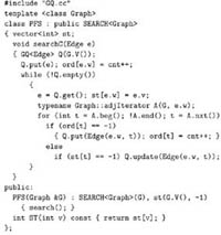
we take them off. The disadvantage of this approach, as with BFS, is that the maximum queue size has to be E instead of V. Or, we could handle updates implicitly in the ADT implementation, just by specifying that no two edges with the same destination vertex can be on the queue. But the simplest way for the ADT implementation to do so is essentially equivalent to using a vertex-indexed vector (see Exercises 4.51 and 4.54), so the test fits more comfortably into the client graph-search program.
The combination of Program 18.10 and the generalized-queue abstraction gives us a general and flexible graph-search mechanism. To illustrate this point, we now consider briefly two interesting and useful alternatives to BFS and DFS.
The first alternative strategy is based on randomized queues (see Section 4.6). In a randomized queue, we remove items randomly: Each item on the data structure is equally likely to be the one removed. Program 18.11 is an implementation that provides this functionality. If we use this code to implement the generalized queue ADT for Program 18.10, then we get a randomized graph-searching algorithm, where each vertex on the fringe is equally likely to be the next one added to the tree. The edge (to that vertex) that is added to the tree depends on the implementation of the update operation. The implementation in Program 18.11 does no updates, so each fringe vertex is added to the tree with the edge that caused it to be moved to the fringe. Alternatively, we might choose to always do updates (which results in the most recently encountered edge to each fringe vertex being added to the tree), or to make a random choice.
Another strategy, which is critical in the study of graph-processing algorithms because it serves as the basis for a number of the classical algorithms that we address in Chapters 20 through 22, is to use a priority-queue ADT (see Chapter 9) for the fringe: We assign priority values to each edge on the fringe, update them as appropriate, and choose the highest-priority edge as the one to be added next to the tree. We consider this formulation in detail in Chapter 20. The queue-maintenance operations for priority queues are more costly than are those for stacks and queues because they involve implicit comparisons among items on the queue, but they can support a much broader class of graph-search algorithms. As we shall see, several critical graph-processing problems can be addressed simply with judicious choice of priority assignments in a priority-queue–based generalized graph search.
All generalized graph-searching algorithms examine each edge just once and take extra space proportional to V in the worst case; they do differ, however, in some performance measures. For example, Figure 18.28 shows the size of the fringe as the search progresses for DFS, BFS, and randomized search; Figure 18.29 shows the tree computed by randomized search for the same example as Figure 18.13 and Figure 18.24. Randomized search has neither the long paths of DFS nor the high-degree nodes of BFS. The shapes of these trees and the fringe plots depend on the structure of the particular graph being searched, but they also characterize the different algorithms.
Figure 18.28 Fringe sizes for DFS, randomized graph search, and BFS
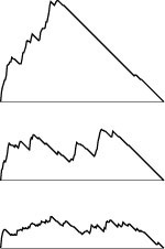
These plots of the fringe size during the searches illustrated in Figures 18.13, 18.24, and 18.29 indicate the dramatic effects that the choice of data structure for the fringe can have on graph searching. When we use a stack, in DFS (top), we fill up the fringe early in the search as we find new nodes at every step, then we end the search by removing everything. When we use a randomized queue (center), the maximum queue size is much lower. When we use a FIFO queue in BFS (bottom), the maximum queue size is still lower, and we discover new nodes throughout the search.
Figure 18.29 Randomized graph search
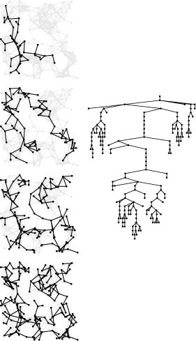
This figure illustrates the progress of randomized graph searching (left), in the same style as Figures 18.13 and 18.24. The search tree shape falls somewhere between the BFS and DFS shapes. The dynamics of these three algorithms, which differ only in the data structure for work to be completed, could hardly be more different.
We could generalize graph searching still further by working with a forest (not necessarily a tree) during the search. Although we stop short of working at this level of generality throughout, we consider a few algorithms of this sort in Chapter 20.
Exercises
• 18.61 Discuss the advantages and disadvantages of a generalized graph-searching implementation that is based on the following policy: “Move an edge from the fringe to the tree. If the vertex that it leads to is unvisited, visit that vertex and put all its incident edges onto the fringe.”
18.62 Develop an adjacency-lists ADT implementation that keeps edges (not just destination vertices) on the lists, then implement a graph search based on the strategy described in Exercise 18.61 that visits every edge but destroys the graph, taking advantage of the fact that you can move all of a vertex’s edges to the fringe with a single link change.
• 18.63 Prove that recursive DFS (Program 18.3) is equivalent to generalized graph search using a stack (Program 18.10), in the sense that both programs will visit all vertices in precisely the same order for all graphs if and only if the programs scan the adjacency lists in opposite orders.
18.64 Give three different possible traversal orders for randomized search through the graph
3-7 1-4 7-8 0-5 5-2 3-8 2-9 0-6 4-9 2-6 6-4.
18.65 Could randomized search visit the vertices in the graph
3-7 1-4 7-8 0-5 5-2 3-8 2-9 0-6 4-9 2-6 6-4
in numerical order of their indices? Prove your answer.
18.66 Use the STL to build a generalized-queue implementation for graph edges that disallows edges with duplicate vertices on the queue, using an ignore-the-new-item policy.
• 18.67 Develop a randomized graph search that chooses each edge on the fringe with equal likelihood. Hint: See Program 18.8.
• 18.68 Describe a maze-traversal strategy that corresponds to using a standard pushdown stack for generalized graph searching (see Section 18.1).
• 18.69 Instrument generalized graph searching (see Program 18.10) to print out the height of the tree and the percentage of edges processed for every vertex to be seen.
• 18.70 Run experiments to determine empirically the average values of the quantities described in Exercise 18.69 for generalized graph search with a random queue in graphs of various sizes, drawn from various graph models (see Exercises 17.64–76).
• 18.71 Implement a derived class that does dynamic graphical animations of generalized graph search for graphs that have (x, y) coordinates associated with each vertex (see Exercises 17.55 through 17.59). Test your program on random Euclidean neighbor graphs, using as many points as you can process in a reasonable amount of time. Your program should produce images like the snapshots shown in Figures 18.13, 18.24, and 18.29, although you should feel free to use colors instead of shades of gray to denote tree, fringe, and unseen vertices and edges.
18.9 Analysis of Graph Algorithms
We have for our consideration a broad variety of graph-processing problems and methods for solving them, so we do not always compare numerous different algorithms for the same problem, as we have in other domains. Still, it is always valuable to gain experience with our algorithms by testing them on real data, or on artificial data that we understand and that have relevant characteristics that we might expect to find in actual applications.
As we discussed briefly in Chapter 2, we seek—ideally—natural input models that have three critical properties:
• They reflect reality to a sufficient extent that we can use them to predict performance.
• They are sufficiently simple that they are amenable to mathematical analysis.
• We can write generators that provide problem instances that we can use to test our algorithms.
With these three components, we can enter into a design-analysis-implementation-test scenario that leads to efficient algorithms for solving practical problems.
For domains such as sorting and searching, we have seen spectacular success along these lines in Parts 3 and 4. We can analyze algorithms, generate random problem instances, and refine implementations to provide extremely efficient programs for use in a host of practical situations. For some other domains that we study, various difficulties can arise. For example, mathematical analysis at the level that we would like is beyond our reach for many geometric problems, and developing an accurate model of the input is a significant challenge for many string-processing algorithms (indeed, doing so is an essential part of the computation). Similarly, graph algorithms take us to a situation where, for many applications, we are on thin ice with respect to all three properties listed in the previous paragraph:
• The mathematical analysis is challenging, and many basic analytic questions remain unanswered.
• There is a huge number of different types of graphs, and we cannot reasonably test our algorithms on all of them.
• Characterizing the types of graphs that arise in practical problems is, for the most part, a poorly understood problem.
Graphs are sufficiently complicated that we often do not fully understand the essential properties of the ones that we see in practice or of the artificial ones that we can perhaps generate and analyze.
The situation is perhaps not as bleak as just described for one primary reason: Many of the graph algorithms that we consider are optimal in the worst case, so predicting performance is a trivial exercise. For example, Program 18.7 finds the bridges after examining each edge and each vertex just once. This cost is the same as the cost of building the graph data structure, and we can confidently predict, for example, that doubling the number of edges will double the running time, no matter what kind of graphs we are processing.
When the running time of an algorithm depends on the structure of the input graph, predictions are much harder to come by. Still, when we need to process huge numbers of huge graphs, we want efficient algorithms for the same reasons that we want them for any other problem domain, and we will continue to pursue the goals of understanding the essential properties of algorithms and applications, striving to identify those methods that can best handle the graphs that might arise in practice.
To illustrate some of these issues, we revisit the study of graph connectivity, a problem that we considered already in Chapter 1 (!). Connectivity in random graphs has fascinated mathematicians for years, and it has been the subject of an extensive literature. That literature is beyond the scope of this book, but it provides a backdrop that validates our use of the problem as the basis for some experimental studies that help us understand the basic algorithms that we use and the types of graphs that we are considering.
For example, growing a graph by adding random edges to a set of initially isolated vertices (essentially, the process behind Program 17.12) is a well-studied process that has served as the basis for
Table 18.1 Connectivity in two random graph models

Key:
C number of connected components
L size of largest connected component
This table shows the number of connected components and the size of the largest connected component for 100000-vertex graphs drawn from two different distributions. For the random graph model, these experiments support the well-known fact that the graph is highly likely to consist primarily of one giant component if the average vertex degree is larger than a small constant. The right two columns give experimental results when we restrict the edges to be chosen from those that connect each vertex to just one of 10 specified neighbors.
classical random graph theory. It is well known that, as the number of edges grows, the graph coalesces into just one giant component. The literature on random graphs gives extensive information about the nature of this process. For example,
Property 18.13 If E > ![]() + µV (with µ positive), a random graph with V vertices and E edges consists of a single connected component and an average of less than e−2µ isolated vertices, with probability approaching 1 as V approaches infinity.
+ µV (with µ positive), a random graph with V vertices and E edges consists of a single connected component and an average of less than e−2µ isolated vertices, with probability approaching 1 as V approaches infinity.
Figure 18.30 Connectivity in random graphs
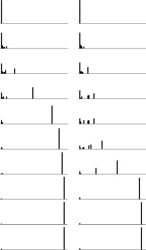
This figures show the evolution of two types of random graphs at 10 equal increments as a total of 2E edges are added to initially empty graphs. Each plot is a histogram of the number of vertices in components of size 1 through V − 1 (left to right). We start out with all vertices in components of size 1 and end with nearly all vertices in a giant component. The plot at left is for a standard random graph: the giant component forms quickly, and all other components are small. The plot at right is for a random neighbor graph: components of various sizes persist for a longer time.
Proof: This fact was established by seminal work of Erdös and Renyi in 1960. The proof is beyond the scope of this book (see reference section).•
This property tells us that we can expect large nonsparse random graphs to be connected. For example, if V > 1000 and E > 10V, then µ > ![]() > 6.5 and the average number of vertices not in the giant component is (almost surely) less than e−13<. 000003. If we generate a million random 1000-vertex graphs of density greater than 10, we might get a few with a single isolated vertex, but the rest will all be connected.
> 6.5 and the average number of vertices not in the giant component is (almost surely) less than e−13<. 000003. If we generate a million random 1000-vertex graphs of density greater than 10, we might get a few with a single isolated vertex, but the rest will all be connected.
Figure 18.30 compares random graphs with random neighbor graphs, where we allow only edges that connect vertices whose indices are within a small constant of one another. The neighbor-graph model yields graphs that are evidently substantially different in character from random graphs. We eventually get a giant component, but it appears suddenly, when two large components merge.
Table 18.2 shows that these structural differences between random graphs and neighbor graphs persist for V and E in ranges of practical interest. Such structural differences certainly may be reflected in the performance of our algorithms.
Table 18.3 gives empirical results for the cost of finding the number of connected components in a random graph, using various algorithms. Although the algorithms perhaps are not subject to direct comparison for this specific task because they are designed to handle different tasks, these experiments do validate a subset of the general conclusions that we have drawn.
First, it is plain from the table that we should not use the adjacency-matrix representation for large sparse graphs (and cannot use it for huge ones), not just because the cost of initializing the matrix is prohibitive, but also because the algorithm inspects every entry in the matrix, so its running time is proportional to the size (V2) of the matrix rather than to the number of 1s in it (E). The table shows, for example, that it takes about as long to process a graph that contains 1000 edges as it does to process one that contains 100000 edges when we are using an adjacency matrix.
Second, it is also plain from Table 18.3 that the cost of allocating memory for the list nodes is significant when we build adjacency lists for large sparse graphs. The cost of building the lists is more than five
Table 18.2 Empirical study of graph-search algorithms
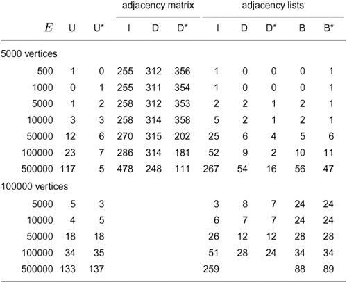
Key:
U weighted quick union with halving (Program 1.4)
I initial construction of the graph representation
D recursive DFS (Program 18.3)
B BFS (Program 18.9)
* exit when graph is found to be fully connected
This table shows relative timings for various algorithms for the task of determining the number of connected components (and the size of the largest one) for graphs with various numbers of vertices and edges. As expected, algorithms that use the adjacency-matrix representation are slow for sparse graphs but competitive for dense graphs. For this specialized task, the union-find algorithms that we considered in Chapter 1 are the fastest, because they build a data structure tailored to solve the problem and do not need otherwise to represent the graph. Once the data structure representing the graph has been built, however, DFS and BFS are faster and more flexible. Adding a test to stop when the graph is known to consist of a single connected component significantly speeds up DFS and union-find (but not BFS) for dense graphs.
times the cost of traversing them. In the typical situation where we are going to perform numerous searches of various types after building the graph, this cost is acceptable. Otherwise, we might consider alternate implementations to reduce this cost.
Third, the absence of numbers in the DFS columns for large sparse graphs is significant. These graphs cause excessive recursion depth, which (eventually) cause the program to crash. If we want to use DFS on such graphs, we need to use the nonrecursive version that we discussed in Section 18.7.
Fourth, the table shows that the union-find–based method from Chapter 1 is faster than DFS or BFS, primarily because it does not have to represent the entire graph. Without such a representation, however, we cannot answer simple queries such as “Is there an edge connecting v and w?” so union-find–based methods are not suitable if we want to do more than what they are designed to do (answer “Is there a path between v and w?” queries intermixed with adding edges). Once the internal representation of the graph has been built, it is not worthwhile to implement a union-find algorithm just to determine whether it is connected, because DFS or BFS can provide the answer about as quickly.
When we run empirical tests that lead to tables of this sort, various anomalies might require further explanation. For example, on many computers, the cache architecture and other features of the memory system might have dramatic impact on performance for large graphs. Improving performance in critical applications may require detailed knowledge of the machine architecture in addition to all the factors that we are considering.
Careful study of these tables will reveal more properties of these algorithms than we are able to address. Our aim is not to do an exhaustive comparison but to illustrate that, despite the many challenges that we face when we compare graph algorithms, we can and should run empirical studies and make use of any available analytic results, both to get a feeling for the algorithms’ important characteristics and to predict performance.
Exercises
• 18.72 Do an empirical study culminating in a table like Table 18.2 for the problem of determining whether or not a graph is bipartite (two-colorable).
18.73 Do an empirical study culminating in a table like Table 18.2 for the problem of determining whether or not a graph is biconnected.
• 18.74 Do an empirical study to find the expected size of the second largest connected component in sparse graphs of various sizes, drawn from various graph models (see Exercises 17.64–76).
18.75 Write a program that produces plots like those in Figure 18.30, and test it on graphs of various sizes, drawn from various graph models (see Exercises 17.64–76).
• 18.76 Modify your program from Exercise 18.75 to produce similar histograms for the sizes of edge-connected components.
••18.77 The numbers in the tables in this section are results for only one sample. We might wish to prepare a similar table where we run 1000 experiments for each entry and give the sample mean and standard deviation, but we probably could not include nearly as many entries. Would this approach be a better use of computer time? Defend your answer.