
CHAPTER NINETEEN
Digraphs and DAGs
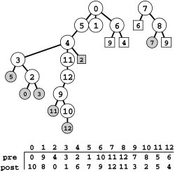
WHEN WE ATTACH significance to the order in which the two vertices are specified in each edge of a graph, we have an entirely different combinatorial object known as a digraph, or directed graph. Figure 19.1 shows a sample digraph. In a digraph, the notation s-t describes an edge that goes from s to t but provides no information about whether or not there is an edge from t to s. There are four different ways in which two vertices might be related in a digraph: no edge; an edge s-t from s to t; an edge t-s from t to s; or two edges s-t and t-s, which indicate connections in both directions. The one-way restriction is natural in many applications, easy to enforce in our implementations, and seems innocuous; but it implies added combinatorial structure that has profound implications for our algorithms and makes working with digraphs quite different from working with undirected graphs. Processing digraphs is akin to traveling around in a city where all the streets are one-way, with the directions not necessarily assigned in any uniform pattern. We can imagine that getting from one point to another in such a situation could be a challenge indeed.
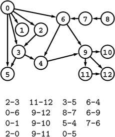
Figure 19.1 A directed graph (digraph)
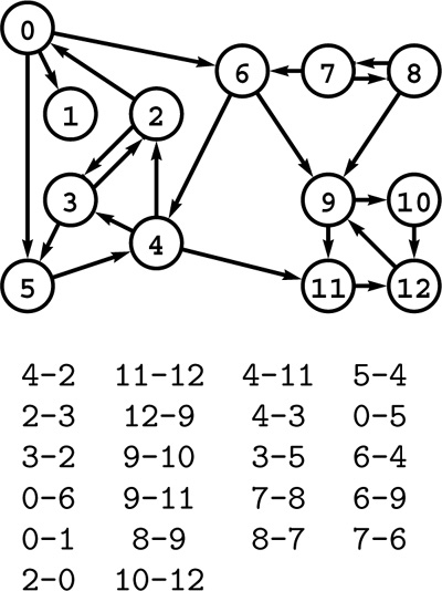
A digraph is defined by a list of nodes and edges (bottom), with the order that we list the nodes when specifying an edge implying that the edge is directed from the first node to the second. When drawing a digraph, we use arrows to depict directed edges (top).
We interpret edge directions in digraphs in many ways. For example, in a telephone-call graph, we might consider an edge to be directed from the caller to the person receiving the call. In a transaction graph, we might have a similar relationship where we interpret an edge as representing cash, goods, or information flowing from one entity to another. We find a modern situation that fits this classic model on the Internet, with vertices representing Web pages and edges the links between the pages. In Section 19.4, we examine other examples, many of which model situations that are more abstract.
One common situation is for the edge direction to reflect a precedence relationship. For example, a digraph might model a manufacturing line: Vertices correspond to jobs to be done, and an edge exists from vertex s to vertex t if the job corresponding to vertex s must be done before the job corresponding to vertex t. Another way to model the same situation is to use a PERT chart: edges represent jobs and vertices implicitly specify the precedence relationships (at each vertex, all incoming jobs must complete before any outgoing jobs can begin). How do we decide when to perform each of the jobs so that none of the precedence relationships are violated? This is known as a scheduling problem. It makes no sense if the digraph has a cycle so, in such situations, we are working with directed acyclic graphs (DAGs). We shall consider basic properties of DAGs and algorithms for this simple scheduling problem, which is known as topological sorting, in Sections 19.5 through 19.7. In practice, scheduling problems generally involve weights on the vertices or edges that model the time or cost of each job. We consider such problems in Chapters 21 and 22.
The number of possible digraphs is truly huge. Each of the V2 possible directed edges (including self-loops) could be present or not, so the total number of different digraphs is 2V2. As illustrated in Figure 19.2, this number grows very quickly, even by comparison with the number of different undirected graphs and even when V is small. As with undirected graphs, there is a much smaller number of classes of digraphs that are isomorphic to each other (the vertices of one can be relabeled to make it identical to the other), but we cannot take advantage of this reduction because we do not know an efficient algorithm for digraph isomorphism.
Figure 19.2 Graph enumeration
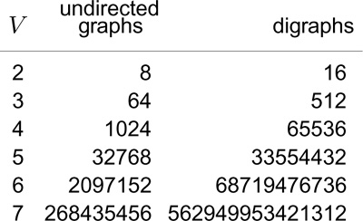
While the number of different undirected graphs with V vertices is huge, even when V is small, the number of different digraphs with V vertices is much larger. For undirected graphs, the number is given by the formula 2V (V +1)/2; for digraphs, the formula is 2V2.
Certainly, any program will have to process only a tiny fraction of the possible digraphs; indeed, the numbers are so large that we can be certain that virtually all digraphs will not be among those processed by any given program. Generally, it is difficult to characterize the digraphs that we might encounter in practice, so we design our algorithms such that they can handle any possible digraph as input. On the one hand, this situation is not new to us (for example, virtually none of the 1000! permutations of 1000 elements have ever been processed by any sorting program). On the other hand, it is perhaps unsettling to know that, for example, even if all the electrons in the universe could run supercomputers capable of processing 1010 graphs per second for the estimated lifetime of the universe, those supercomputers would see far fewer than 10−100 percent of the 10-vertex digraphs (see Exercise 19.9).
This brief digression on graph enumeration perhaps underscores several points that we cover whenever we consider the analysis of algorithms and indicates their particular relevance to the study of digraphs. Is it important to design our algorithms to perform well in the worst case, when we are so unlikely to see any particular worst-case digraph? Is it useful to choose algorithms on the basis of average-case analysis, or is that a mathematical fiction? If our intent is to have implementations that perform efficiently on digraphs that we see in practice, we are immediately faced with the problem of characterizing those digraphs. Mathematical models that can convincingly describe the digraphs that we might expect in applications are even more difficult to develop than are models for undirected graphs.
In this chapter, we revisit, in the context of digraphs, a subset of the basic graph-processing problems that we considered in Chapter 17, and we examine several problems that are specific to digraphs. In particular, we look at DFS and several of its applications, including cycle detection (to determine whether a digraph is a DAG);topological sort (to solve, for example, the scheduling problem for DAGs that was just described); and computation of the transitive closure and the strong components (which have to do with the basic problem of determining whether or not there is a directed path between two given vertices). As in other graph-processing domains, these algorithms range from the trivial to the ingenious; they are both informed by and give us insight into the complex combinatorial structure of digraphs.
Exercises
• 19.1 Find a large digraph somewhere online—perhaps a transaction graph in some online system, or a digraph defined by links on Web pages.
• 19.2 Find a large DAG somewhere online—perhaps one defined by function-definition dependencies in a large software system, or by directory links in a large file system.
19.3 Make a table like Figure 19.2, but exclude from the counts graphs and digraphs with self-loops.
19.4 How many digraphs are there that contain V vertices and E edges?
• 19.5 How many digraphs correspond to each undirected graph that contains V vertices and E edges?
• 19.6 How many digits do we need to express the number of digraphs that have V vertices as a base-10 number?
• 19.7 Draw the nonisomorphic digraphs that contain three vertices.
••• 19.8 How many different digraphs are there with V vertices and E edges if we consider two digraphs to be different only if they are not isomorphic?
• 19.9 Compute an upper bound on the percentage of 10-vertex digraphs that could ever be examined by any computer, under the assumptions described in the text and the additional ones that the universe has less than 1080 electrons and that the age of the universe will be less than 1020 years.
19.1 Glossary and Rules of the Game
Our definitions for digraphs are nearly identical to those in Chapter 17 for undirected graphs (as are some of the algorithms and programs that we use), but they are worth restating. The slight differences in the wording to account for edge directions imply structural properties that will be the focus of this chapter.
Definition 19.1 A digraph (or directed graph ) is a set of vertices plus a set of directed edges that connect ordered pairs of vertices (with no duplicate edges). We say that an edge goes from its first vertex to its second vertex.
As we did with undirected graphs, we disallow duplicate edges in this definition but reserve the option of allowing them when convenient for various applications and implementations. We explicitly allow self-loops in digraphs (and usually adopt the convention that every vertex has one) because they play a critical role in the basic algorithms.
Definition 19.2 A directed path in a digraph is a list of vertices in which there is a (directed) digraph edge connecting each vertex in the list to its successor in the list. We say that a vertex t is reachable from a vertex s if there is a directed path from s to t.
We adopt the convention that each vertex is reachable from itself and normally implement that assumption by ensuring that self-loops are present in our digraph representations.
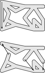
Understanding many of the algorithms in this chapter requires understanding the connectivity properties of digraphs and the effect of these properties on the basic process of moving from one vertex to another along digraph edges. Developing such an understanding is more complicated for digraphs than for undirected graphs. For example, we might be able to tell at a glance whether a small undirected graph is connected or contains a cycle; these properties are not as easy to spot in digraphs, as indicated in the typical example illustrated in Figure 19.3.
Figure 19.3 A grid digraph
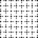
This small digraph is similar to the large grid network that we first considered in Chapter 1, except that it has a directed edge on every grid line, with the direction randomly chosen. Even though the graph has relatively few nodes, its connectivity properties are not readily apparent. Is there a directed path from the upper left corner to the lower right corner?
While examples like this highlight differences, it is important to note that what a human considers difficult may or may not be relevant to what a program considers difficult—for instance, writing a DFS class to find cycles in digraphs is no more difficult than for undirected graphs. More important, digraphs and graphs have essential structural differences. For example, the fact that t is reachable from s in a digraph indicates nothing about whether s is reachable from t. This distinction is obvious, but critical, as we shall see.
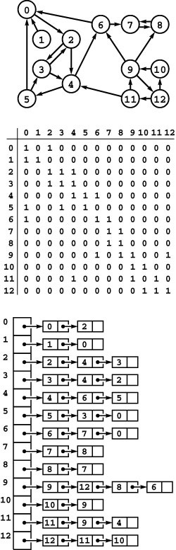
As mentioned in Section 17.3, the representations that we use for digraphs are essentially the same as those that we use for undirected graphs. Indeed, they are more straightforward because we represent each edge just once, as illustrated in Figure 19.4. In the adjacency-lists representation, an edge s-t is represented as a list node containing t in the linked list corresponding to s. In the adjacency-matrix representation, we need to maintain a full V -by-V matrix and to represent an edge s-t by a 1 bit in row s and column t. We do not put a 1 bit in row t and column s unless there is also an edge t-s. In general, the adjacency matrix for a digraph is not symmetric about the diagonal.
Figure 19.4 Digraph representations
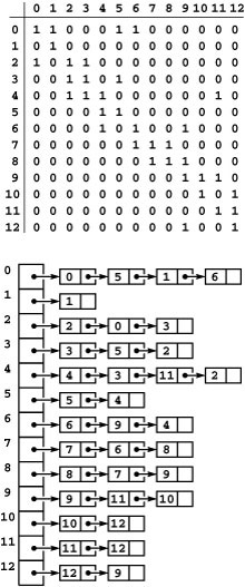
The adjacency-matrix and adjacency-lists representations of a digraph have only one representation of each edge, as illustrated in the adjacency-matrix (top) and adjacency-lists (bottom) representation of the graph depicted in Figure 19.1. These representations both include self-loops at every vertex, which is typical in digraph processing.
There is no difference in these representations between an undirected graph and a directed graph with self-loops at every vertex and two directed edges for each edge connecting distinct vertices in the undirected graph (one in each direction). Thus, we can use the algorithms that we develop in this chapter for digraphs to process undirected graphs, provided that we interpret the results appropriately. In addition, we use the programs that we considered in Chapter 17 as the basis for our digraph programs: Our DenseGRAPH and SparseMultiGRAPH class implementations Programs 17.7 through 17.10 build digraphs when the constructor has true as a second argument.
The indegree of a vertex in a digraph is the number of directed edges that lead to that vertex. The outdegree of a vertex in a digraph is the number of directed edges that emanate from that vertex. No vertex is reachable from a vertex of outdegree 0, which is called a sink; a vertex of indegree 0, which is called a source, is not reachable from any other vertex. A digraph where self-loops are allowed and every vertex has outdegree 1 is called a map (a function from the set of integers from 0 to V − 1 onto itself). We can easily compute the indegree and outdegree of each vertex, and find sources and sinks, in linear time and space proportional to V, using vertex-indexed vectors (see Exercise 19.19).
The reverse of a digraph is the digraph that we obtain by switching the direction of all the edges. Figure 19.5 shows the reverse and its representations for the digraph of Figure 19.1. We use the reverse in digraph algorithms when we need to know from where edges come because our standard representations tell us only where the edges go. For example, indegree and outdegree change roles when we reverse a digraph.
Figure 19.5 Digraph reversal
Reversing the edges of a digraph corresponds to transposing the adjacency matrix but requires rebuilding the adjacency lists (see Figures 19.1 and 19.4).
For an adjacency-matrix representation, we could compute the reverse by making a copy of the matrix and transposing it (interchanging its rows and columns). If we know that the graph is not going to be modified, we can actually use the reverse without any extra computation by simply interchanging the vertices in our references to edges when we want to refer to the reverse. For example, an edge s-t in a digraph G is indicated by a 1 in adj[s][t]. Thus, if we were to compute the reverse R of G, it would have a 1 in adj[t][s]. We do not need to do so, however, if we base our client implementations on the edge test edge(s, t), because to switch to the reverse we just replace every such reference by edge(t, s). This opportunity may seem obvious, but it is often overlooked. For an adjacency-lists representation, the reverse is a completely different data structure, and we need to take time proportional to the number of edges to build it, as shown in Program 19.1.
Yet another option, which we shall address in Chapter 22, is to maintain two representations of each edge, in the same manner as we do for undirected graphs (see Section 17.3) but with an extra bit that indicates edge direction. For example, to use this method in an adjacency-lists representation we would represent an edge s-t by a node for t on the adjacency list for s (with the direction bit set to indicate that to move from s to t is a forward traversal of the edge) and a node for s on the adjacency list for t (with the direction bit set to indicate that to move from t to s is a backward traversal of the edge). This representation supports algorithms that need to traverse edges in digraphs in both directions. It is also generally convenient to include pointers connecting the two representations of each edge in such cases. We defer considering this representation in detail to Chapter 22, where it plays an essential role.
In digraphs, by analogy to undirected graphs, we speak of directed cycles, which are directed paths from a vertex back to itself, and simple directed paths and cycles, where the vertices and edges are distinct. Note that s-t-s is a cycle of length 2 in a digraph but that cycles in undirected graphs must have at least three distinct vertices.
In many applications of digraphs, we do not expect to see any cycles, and we work with yet another type of combinatorial object.
Definition 19.3A directed acyclic graph (DAG) is a digraph with no directed cycles.
We expect DAGs, for example, in applications where we are using digraphs to model precedence relationships. DAGs not only arise naturally in these and other important applications, but also, as we shall see, in the study of the structure of general digraphs. A sample DAG is illustrated in Figure 19.6.
Figure 19.6 A directed acyclic graph (DAG)
This digraph has no cycles, a property that is not immediately apparent from the edge list or even from examining its drawing.
Directed cycles are therefore the key to understanding connectivity in digraphs that are not DAGs. An undirected graph is connected if there is a path from every vertex to every other vertex; for digraphs, we modify the definition as follows:
Definition 19.4 A digraph is strongly connected if every vertex is reachable from every vertex.
The graph in Figure 19.1 is not strongly connected because, for example, there are no directed paths from vertices 9 through 12 to any of the other vertices in the graph.
As indicated by strongly, this definition implies a relationship between each pair of vertices stronger than reachability. In any digraph, we say that a pair of vertices s and t are strongly connected or mutually reachable if there is a directed path from s to t and a directed path from t to s. (Our convention that each vertex is reachable from itself implies that each vertex is strongly connected to itself.) A digraph is strongly connected if and only if all pairs of vertices are strongly connected. The defining property of strongly connected digraphs is one that we take for granted in connected undirected graphs: If there is a path from s to t, then there is a path from t to s. In the case of undirected graphs, we know this fact because the same path fits the bill, traversed in the other direction; in digraphs, it must be a different path.
Another way of saying that a pair of vertices is strongly connected is that they lie on some directed cyclic path. Recall that we use the term cyclic path instead of cycle to indicate that the path does not need to be simple. For example, in Figure 19.1, 5 and 6 are strongly connected because 6 is reachable from 5 via the directed path 5-4-2-0-6 and 5 is reachable from 6 via the directed path 6-4-3-5; and these paths imply that 5 and 6 lie on the directed cyclic path 5-4-2-0-6-4-3-5, but they do not lie on any (simple) directed cycle. Note that no DAG that contains more than one vertex is strongly connected.
Like simple connectivity in undirected graphs, this relation is transitive: If s is strongly connected to t, and t is strongly connected to u, then s is strongly connected to u. Strong connectivity is an equivalence relation that divides the vertices into equivalence classes containing vertices that are strongly connected to each other. (See Section 19.4 for a detailed discussion of equivalence relations.) Again, strong connectivity provides a property for digraphs that we take for granted with respect to connectivity in undirected graphs.
Figure 19.7 Digraph terminology
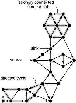
Sources (vertices with no edges coming in) and sinks (vertices with no edges going out) are easy to identify in digraph drawings like this one, but directed cycles and strongly connected components are more difficult to identify. What is the longest directed cycle in this digraph? How many strongly connected components with more than one vertex are there?
Property 19.1 A digraph that is not strongly connected comprises a set of strongly connected components ( strong components , for short), which are maximal strongly connected subgraphs, and a set of directed edges that go from one component to another.
Proof: Like components in undirected graphs, strong components in digraphs are induced subgraphs of subsets of vertices: Each vertex is in exactly one strong component. To prove this fact, we first note that every vertex belongs to at least one strong component, which contains (at least) the vertex itself. Then we note that every vertex belongs to at most one strong component: If a vertex were to belong to two different components, then there would be paths through that vertex connecting vertices in those components to each other, in both directions, which contradicts the maximality of both components.
For example, a digraph that consists of a single directed cycle has just one strong component. At the other extreme, each vertex in a DAG is a strong component, so each edge in a DAG goes from one component to another. In general, not all edges in a digraph are in the strong components. This situation is in contrast to the analogous situation for connected components in undirected graphs, where every vertex and every edge belongs to some connected component, but similar to the analogous situation for edge-connected components in undirected graphs. The strong components in a digraph are connected by edges that go from a vertex in one component to a vertex in another but do not go back again.
Property 19.2 Given a digraph D, define another digraph K ( D ) with one vertex corresponding to each strong component of D and one edge in K ( D ) corresponding to each edge in D that connects vertices in different strong components (connecting the vertices in K that correspond to the strong components that it connects in D). Then, K ( D ) is a DAG (which we call the kernel DAG of D).
Proof: If K ( D ) were to have a directed cycle, then vertices in two different strong components of D would fall on a directed cycle, and that would be a contradiction.
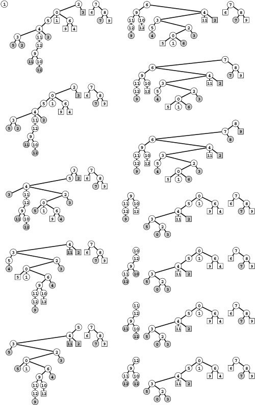
Figure 19.8 shows the strong components and the kernel DAG for a sample digraph. We look at algorithms for finding strong components and building kernel DAGs in Section 19.6.
Figure 19.8 Strong components and kernel DAG
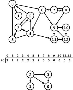
This digraph (top) consists of four strong components, as identified (with arbitrary integer labels) by the vertex-indexed array id (center). Component 0 consists of the vertices 9, 10, 11 and 12; component 1 consists of the single vertex 1; component 2 consists of the vertices 0, 2, 3, 4, 5, and 6; and component 3 consists of the vertices 7 and 8. If we draw the graph defined by the edges between different components, we get a DAG (bottom).
From these definitions, properties, and examples, it is clear that we need to be precise when referring to paths in digraphs. We need to consider at least the following three situations:
Connectivity We reserve the term connected for undirected graphs. In digraphs, we might say that two vertices are connected if they are connected in the undirected graph defined by ignoring edge directions, but we generally avoid such usage.
Reachability In digraphs, we say that vertex t is reachable from vertex s if there is a directed path from s to t. We generally avoid the term reachable when referring to undirected graphs, although we might consider it to be equivalent to connected because the idea of one vertex being reachable from another is intuitive in certain undirected graphs (for example, those that represent mazes).
Strong connectivity Two vertices in a digraph are strongly connected if they are mutually reachable; in undirected graphs, two connected vertices imply the existence of paths from each to the other. Strong connectivity in digraphs is similar in certain ways to edge connectivity in undirected graphs.
We wish to support digraph ADT operations that take two vertices s and t as arguments and allow us to test whether
• t is reachable from s
• s and t are strongly connected (mutually reachable)
What resource requirements are we willing to expend for these operations? As we saw in Section 17.5, DFS provides a simple solution for connectivity in undirected graphs that takes time proportional to V, but if we are willing to invest preprocessing time proportional to V + E and space proportional to V, we can answer connectivity queries in constant time. Later in this chapter, we examine algorithms for strong connectivity that have these same performance characteristics.
But our primary aim is to address the fact that reachability queries in digraphs are more difficult to handle than connectivity or strong connectivity queries. In this chapter, we examine classical algorithms that require preprocessing time proportional to V E and space proportional to V2, develop implementations that can achieve constant-time reachability queries with linear space and preprocessing time for some di-graphs, and study the difficulty of achieving this optimal performance for all digraphs.
Exercises
• 19.10 Give the adjacency-lists structure that is built by Program 17.9 for the digraph
3-7 1-4 7-8 0-5 5-2 3-8 2-9 0-6 4-9 2-6 6-4.
• 19.11 Write a program to generate random sparse digraphs for a well-chosen set of values of V and E such that you can use it to run meaningful empirical tests on digraphs drawn from the random-edges model.
• 19.12 Write a program to generate random sparse graphs for a well-chosen set of values of V and E such that you can use it to run meaningful empirical tests on graphs drawn from the random-graph model.
• 19.13 Write a program that generates random digraphs by connecting vertices arranged in a ![]() -by-
-by- ![]() grid to their neighbors, with edge directions randomly chosen (see Figure 19.3).
grid to their neighbors, with edge directions randomly chosen (see Figure 19.3).
• 19.14 Augment your program from Exercise 19.13 to add R extra random edges (all possible edges equally likely). For large R, shrink the grid so that the total number of edges remains about V. Test your program as described in Exercise 19.11.
• 19.15 Modify your program from Exercise 19.14 such that an extra edge goes from a vertex s to a vertex t with probability inversely proportional to the Euclidean distance between s and t.
• 19.16 Write a program that generates V random intervals in the unit interval, all of length d, then builds a digraph with an edge from interval s to interval t if and only if at least one of the endpoints of s falls within t (see Exercise 17.75). Determine how to set d so that the expected number of edges is E. Test your program as described in Exercise 19.11 (for low densities) and as described in Exercise 19.12 (for high densities).
• 19.17 Write a program that chooses V vertices and E edges from the real digraph that you found for Exercise 19.1. Test your program as described in Exercise 19.11 (for low densities) and as described in Exercise 19.12 (for high densities).
• 19.18 Write a program that produces each of the possible digraphs with V vertices and E edges with equal likelihood (see Exercise 17.70). Test your program as described in Exercise 19.11 (for low densities) and as described in Exercise 19.12 (for high densities).
• 19.19 Implement a class that provides clients with the capability to learn the indegree and outdegree of any given vertex in a digraph, in constant time, after linear-time preprocessing in the constructor. Then add member functions that return the number of sources and sinks, in constant time.
• 19.20 Use your program from Exercise 19.19 to find the average number of sources and sinks in various types of digraphs (see Exercises 19.11–18).
• 19.21 Show the adjacency-lists structure that is produced when you use Program 19.1 to find the reverse of the digraph
3-7 1-4 7-8 0-5 5-2 3-8 2-9 0-6 4-9 2-6 6-4.
• 19.22 Characterize the reverse of a map.
19.23 Design a digraph class that explicitly provides clients with the capability to refer to both a digraph and its reverse, and provide an implementation, for any representation that supports edge queries.
19.24 Provide an alternate implementation for your class in Exercise 19.23 that maintains both orientations of edges on adjacency lists.
• 19.25 Describe a family of strongly connected digraphs with V vertices and no (simple) directed cycles of length greater than 2.
• 19.26 Give the strong components and a kernel DAG of the digraph
3-7 1-4 7-8 0-5 5-2 3-8 2-9 0-6 4-9 2-6 6-4.
• 19.27 Give a kernel DAG of the grid digraph shown in Figure 19.3.
19.28 How many digraphs have V vertices, all of outdegree k?
• 19.29 What is the expected number of different adjacency-lists representations of a random digraph? Hint: Divide the total number of possible representations by the total number of digraphs.
19.2 Anatomy of DFS in Digraphs
We can use our DFS code for undirected graphs from Chapter 18 to visit each edge and each vertex in a digraph. The basic principle behind the recursive algorithm holds: To visit every vertex that can be reached from a given vertex, we mark the vertex as having been visited, then (recursively) visit all the vertices that can be reached from each of the vertices on its adjacency list.
In an undirected graph, we have two representations of each edge, but the second representation that is encountered in a DFS always leads to a marked vertex and is ignored (see Section 18.2). In a digraph, we have just one representation of each edge, so we might expect DFS algorithms to be more straightforward. But digraphs themselves are more complicated combinatorial objects than undirected graphs, so this expectation is not justified. For example, the search trees that we use to understand the operation of the algorithm have a more complicated structure for digraphs than for undirected graphs. This complication makes digraph-processing algorithms more difficult to devise. For example, as we will see, it is more difficult to make inferences about directed paths in digraphs than it is to make inferences about paths in graphs.
As we did in Chapter 18, we use the term standard adjacency-lists DFS to refer to the process of inserting a sequence of edges into a digraph ADT implemented with an adjacency-lists representation (Program 17.9, invoked with true as the constructor’s second argument), then doing a DFS with, for example, Program 18.3 and the parallel term standard adjacency-matrix DFS to refer to the process of inserting a sequence of edges into a digraph ADT implemented with an adjacency-matrix representation (Program 17.7, invoked with true as the constructor’s second argument), then doing a DFS with, for example, Program 18.3.
For example, Figure 19.9 shows the recursive-call tree that describes the operation of a standard adjacency-lists DFS on the sample digraph in Figure 19.1. Just as for undirected graphs, such trees have internal nodes that correspond to calls on the recursive DFS function for each vertex, with links to external nodes that correspond to edges that take us to vertices that have already been seen. Classifying the nodes and links gives us information about the search (and the di-graph), but the classification for digraphs is quite different from the classification for undirected graphs.
Figure 19.9 DFS forest for a digraph
This forest describes a standard adjacency-lists DFS of the sample digraph in Figure 19.1. External nodes represent previously visited internal nodes with the same label; otherwise the forest is a representation of the digraph, with all edges pointing down. There are four types of edges: tree edges, to internal nodes; back edges, to external nodes representing ancestors (shaded circles); down edges, to external nodes representing descendants (shaded squares); and cross edges, to external nodes representing nodes that are neither ancestors nor descendants (white squares). We can determine the type of edges to visited nodes, by comparing the preorder and postorder numbers (bottom) of their source and destination:
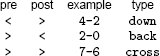
For example, 7-6 is a cross edge because 7‘s preorder and postorder numbers are both larger than 6’s.
In undirected graphs, we assigned each link in the DFS tree to one of four classes according to whether it corresponded to a graph edge that led to a recursive call and to whether it corresponded to the first or second representation of the edge encountered by the DFS. In digraphs, there is a one-to-one correspondence between tree links and graph edges, and they fall into four distinct classes:
• Those representing a recursive call ( tree edges)
• Those from a vertex to an ancestor in its DFS tree ( back edges)
• Those from a vertex to a descendant in its DFS tree ( down edges)
• Those from a vertex to another vertex that is neither an ancestor nor a descendant in its DFS tree ( cross edges)
A tree edge is an edge to an unvisited vertex, corresponding to a recursive call in the DFS. Back, cross, and down edges go to visited vertices. To identify the type of a given edge, we use preorder and postorder numbering (the order in which nodes are visited in preorder and postorder walks of the forest, respectively).
Property 19.3 In a DFS forest corresponding to a digraph, an edge to a visited node is a back edge if it leads to a node with a higher postorder number; otherwise, it is a cross edge if it leads to a node with a lower preorder number and a down edge if it leads to a node with a higher preorder number.
Proof: These facts follow from the definitions. A node’s ancestors in a DFS tree have lower preorder numbers and higher postorder numbers; its descendants have higher preorder numbers and lower postorder numbers. It is also true that both numbers are lower in previously visited nodes in other DFS trees, and both numbers are higher in yetto-be-visited nodes in other DFS trees, but we do not need code that tests for these cases.
Program 19.2 is a DFS class that identifies the type of each edge in the digraph. Figure 19.10 illustrates its operation on the example digraph of Figure 19.1. During the search, testing to see whether an edge leads to a node with a higher postorder number is equivalent to testing whether a postorder number has yet been assigned. Any node for which a preorder number has been assigned but for which a postorder number has not yet been assigned is an ancestor in the DFS tree and will therefore have a postorder number higher than that of the current node.
Figure 19.10 Digraph DFS trace
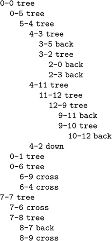
This DFS trace is the output of Program 19.2 for the example digraph in Figure 19.1. It corresponds precisely to a preorder walk of the DFS tree depicted in Figure 19.9.
As we saw in Chapter 17 for undirected graphs, the edge types are properties of the dynamics of the search, rather than of only the graph. Indeed, different DFS forests of the same graph can differ remarkably in character, as illustrated in Figure 19.11. For example, even the number of trees in the DFS forest depends upon the start vertex.
Despite these differences, several classical digraph-processing algorithms are able to determine digraph properties by taking appropriate action when they encounter the various types of edges during a DFS. For example, consider the following basic problem:
Directed cycle detection Does a given digraph have any directed cycles? (Is the digraph a DAG?) In undirected graphs, any edge to a visited vertex indicates a cycle in the graph; in digraphs, we must restrict our attention to back edges.
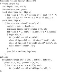
Program 19.2 DFS of a digraph
This DFS class uses preorder and postorder numberings to show the role that each edge in the graph plays in the DFS (see Figure 19.10).
Property 19.4 A digraph is a DAG if and only if we encounter no back edges when we use DFS to examine every edge.
Proof: Any back edge belongs to a directed cycle that consists of the edge plus the tree path connecting the two nodes, so we will find no back edges when using DFS on a DAG. To prove the converse, we show that if the digraph has a cycle, then the DFS encounters a back
Figure 19.11 DFS forests for a digraph
These forests describes depth-first search of the same graph as Figure 19.9, when the graph search function checks the vertices (and calls the recursive function for the unvisited ones) in the order s, s+1, …, V-1, 0, 1, …, s-1 for each s. The forest structure is determined both by the search dynamics and the graph structure. Each node has the same children (the nodes on its adjacency list, in order) in every forest. The leftmost tree in each forest contains all the nodes reachable from its root, but reachability inferences about other nodes are complicated because of back, cross, and down edges. Even the number of trees in the forest depends on the starting node, so we do not necessarily have a direct correspondence between trees in the forest and strong components, the way that we did for components in undirected graphs. For example, we see that all vertices are reachable from 8 only when we start the DFS at 8.
edge. Suppose that v is the first of the vertices on the cycle that is visited by the DFS. That vertex has the lowest preorder number of all the vertices on the cycle. The edge that points to it will therefore be a back edge: It will be encountered during the recursive call for v (for a proof that it must be, see Property 19.5), and it points from some node on the cycle to v, a node with a lower preorder number (see Property 19.3).
We can convert any digraph into a DAG by doing a DFS and removing any graph edges that correspond to back edges in the DFS. For example, Figure 19.9 tells us that removing the edges 2-0, 3-5, 2-3, 9-11, 10-12, 4-2, and 8-7 makes the digraph in Figure 19.1 a DAG. The specific DAG that we get in this way depends on the graph representation and the associated implications for the dynamics of the DFS (see Exercise 19.37). This method is a useful way to generate large arbitrary DAGs randomly (see Exercise 19.76) for use in testing DAG-processing algorithms.
Directed cycle detection is a simple problem, but contrasting the solution just described with the solution that we considered in Chapter 18 for undirected graphs gives insight into the necessity of considering the two types of graphs as different combinatorial objects, even though their representations are similar and the same programs work on both types for some applications. By our definitions, we seem to be using the same method to solve this problem as for cycle detection in undirected graphs (look for back edges), but the implementation that we used for undirected graphs would not work for digraphs. For example, in Section 18.5 we were careful to distinguish between parent links and back links since the existence of a parent link does not indicate a cycle (cycles in undirected graphs must involve at least three vertices). But to ignore links back to a node’s parents in digraphs would be incorrect; we do consider a doubly-connected pair of vertices in a digraph to be a cycle. Theoretically, we could have defined back edges in undirected graphs in the same way as we have done here, but then we would have needed an explicit exception for the two-vertex case. More important, we can detect cycles in undirected graphs in time proportional to V (see Section 18.5), but we may need time proportional to E to find a cycle in a digraph (see Exercise 19.32).
The essential purpose of DFS is to provide a systematic way to visit all the vertices and all the edges of a graph. It therefore gives us a basic approach for solving reachability problems in digraphs, although, again, the situation is more complicated than for undirected graphs.
Single-source reachability Which vertices in a given digraph can be reached from a given start vertex s? How many such vertices are there?
Property 19.5 With a recursive DFS starting at s, we can solve the single-source reachability problem for a vertex s in time proportional to the number of edges in the subgraph induced by the reachable vertices.
Proof: This proof is essentially the same as the proof of Property 18.1, but it is worth restating to underline the distinction between reachability in digraphs and connectivity in undirected graphs. The property is certainly true for a digraph that has one vertex and no edges. For any digraph that has more than one vertex, we assume the property to be true for all digraphs that have fewer vertices. Now, the first edge that we take from s divides the digraph into the subgraphs induced by two subsets of vertices (see Figure 19.12): ( i ) the vertices that we can reach by directed paths that begin with that edge and do not otherwise include s;and( ii ) the vertices that we cannot reach with a directed path that begins with that edge without returning to s. We apply the inductive hypothesis to these subgraphs, noting that there are no directed edges from a vertex in the first subgraph to any vertex other than s in the second subgraph (such an edge would be a contradiction because its destination vertex should be in the first subgraph), that directed edges to s will be ignored because it has the lowest preorder number, and that all the vertices in the first subgraph have lower preorder numbers than any vertex in the second subgraph, so all directed edges from a vertex in the second subgraph to a vertex in the first subgraph will be ignored.
Figure 19.12 Decomposing a digraph
To prove by induction that DFS takes us everywhere reachable from a given node in a digraph, we use essentially the same proof as for Trémaux exploration. The key step is depicted here as a maze (top), for comparison with Figure 18.4. We break the graph into two smaller pieces (bottom), induced by two sets of vertices: Those vertices that can be reached by following the first edge from the start vertex without revisiting it (bottom piece), and those vertices that cannot be reached by following the first edge without going back through the start vertex (top piece). Any edge that goes from a vertex in the first set to the start vertex is skipped during the search of the first set because of the mark on the start vertex. Any edge that goes from a vertex in the second set to a vertex in the first set is skipped because all vertices in the first set are marked before the search of the second subgraph begins.
By contrast with undirected graphs, a DFS on a digraph does not give full information about reachability from any vertex other than the start node, because tree edges are directed and because the search structures have cross edges. When we leave a vertex to travel down a tree edge, we cannot assume that there is a way to get back to that vertex via digraph edges; indeed, there is not, in general. For example, there is no way to get back to 4 after we take the tree edge 4-11 in Figure 19.9. Moreover, when we ignore cross and forward edges (because they lead to vertices that have been visited and are no longer active), we are ignoring information that they imply (the set of vertices that are reachable from the destination). For example, following the cross edge 6-9 in Figure 19.9 is the only way for us to find out that 10, 11, and 12 are reachable from 6.
To determine which vertices are reachable from another vertex, we apparently need to start over with a new DFS from that vertex (see Figure 19.11). Can we make use of information from previous searches to make the process more efficient for later ones? We consider such reachability questions in Section 19.7.
To determine connectivity in undirected graphs, we rely on knowing that vertices are connected to their ancestors in the DFS tree, through (at least) the path in the tree. By contrast, the tree path goes in the wrong direction in a digraph: There is a directed path from a vertex in a digraph to an ancestor only if there is a back edge from a descendant to that or a more distant ancestor. Moreover, connectivity in undirected graphs for each vertex is restricted to the DFS tree rooted at that vertex; in contrast, in digraphs, cross edges can take us to any previously visited part of the search structure, even one in another tree in the DFS forest. For undirected graphs, we were able to take advantage of these properties of connectivity to identify each vertex with a connected component in a single DFS, then to use that information as the basis for a constant-time ADT operation to determine whether any two vertices are connected. For digraphs, as we see in this chapter, this goal is elusive.
We have emphasized throughout this and the previous chapter that different ways of choosing unvisited vertices lead to different search dynamics for DFS. For digraphs, the structural complexity of the DFS trees leads to differences in search dynamics that are even more pronounced than those we saw for undirected graphs. For example, Figure 19.11 illustrates that we get marked differences for digraphs even when we simply vary the order in which the vertices are examined in the top-level search function. Only a tiny fraction of even these possibilities is shown in the figure—in principle, each of the V ! different orders of examining vertices might lead to different results. In Section 19.7, we shall examine an important algorithm that specifically takes advantage of this flexibility, processing the unvisited vertices at the top level (the roots of the DFS trees) in a particular order that immediately exposes the strong components.
Exercises
19.30 Draw the DFS forest that results from a standard adjacency-lists DFS of the digraph
3-7 1-4 7-8 0-5 5-2 3-8 2-9 0-6 4-9 2-6 6-4.
19.31 Draw the DFS forest that results from a standard adjacency-matrix DFS of the digraph
3-7 1-4 7-8 0-5 5-2 3-8 2-9 0-6 4-9 2-6 6-4.
• 19.32 Describe a family of digraphs with V vertices and E edges for which a standard adjacency-lists DFS requires time proportional to E for cycle detection.
• 19.33 Show that, during a DFS in a digraph, no edge connects a node to another node whose preorder and postorder numbers are both smaller.
• 19.34 Show all possible DFS forests for the digraph
0-1 0-2 0-3 1-3 2-3.
Tabulate the number of tree, back, cross, and down edges for each forest.
19.35 If we denote the number of tree, back, cross, and down edges by t, b, c, and d, respectively, then we have t + b + c + d = E and t < V for any DFS of any digraph with V vertices and E edges. What other relationships among these variables can you infer? Which of the values are dependent solely on graph properties, and which are dependent on dynamic properties of the DFS?
• 19.36 Prove that every source in a digraph must be a root of some tree in the forest corresponding to any DFS of that digraph.
• 19.37 Construct a connected DAG that is a subgraph of Figure 19.1 by removing five edges (see Figure 19.11).
19.38 Implement a digraph class that provides the capability for a client to check that a digraph is indeed a DAG, and provide a DFS-based implementation.
19.39 Use your solution to Exercise 19.38 to estimate (empirically) the probability that a random digraph with V vertices and E edges is a DAG for various types of digraphs (see Exercises 19.11–18).
19.40 Run empirical studies to determine the relative percentages of tree, back, cross, and down edges when we run DFS on various types of digraphs (see Exercises 19.11–18).
19.41 Describe how to construct a sequence of directed edges on V vertices for which there will be no cross or down edges and for which the number of back edges will be proportional to V2 in a standard adjacency-lists DFS.
• 19.42 Describe how to construct a sequence of directed edges on V vertices for which there will be no back or down edges and for which the number of cross edges will be proportional to V2 in a standard adjacency-lists DFS.
19.43 Describe how to construct a sequence of directed edges on V vertices for which there will be no back or cross edges and for which the number of down edges will be proportional to V2 in a standard adjacency-lists DFS.
• 19.44 Give rules corresponding to Trémaux traversal for a maze where all the passages are one-way.
• 19.45 Extend your solutions to Exercises 17.56 through 17.60 to include arrows on edges (see the figures in this chapter for examples).
19.3 Reachability and Transitive Closure
To develop efficient solutions to reachability problems in digraphs, we begin with the following fundamental definition.
Definition 19.5 The transitive closure of a digraph is a digraph with the same vertices but with an edge from s to t in the transitive closure if and only if there is a directed path from s to t in the given digraph.
In other words, the transitive closure has an edge from each vertex to all the vertices reachable from that vertex in the digraph. Clearly, the transitive closure embodies all the requisite information for solving reachability problems. Figure 19.13 illustrates a small example.
Figure 19.13 Transitive closure
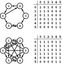
This digraph (top) has just eight directed edges, but its transitive closure (bottom) shows that there are directed paths connecting 19 of the 30 pairs of vertices. Structural properties of the digraph are reflected in the transitive closure. For example, rows 0, 1, and 2 in the adjacency matrix for the transitive closure are identical (as are columns 0, 1, and 2) because those vertices are on a directed cycle in the digraph.
One appealing way to understand the transitive closure is based on adjacency-matrix digraph representations, and on the following basic computational problem.
Boolean matrix multiplication A Boolean matrix is a matrix whose entries are all binary values, either 0 or 1. Given two Boolean matrices A and B, compute a Boolean product matrix C, using the logical and and or operations instead of the arithmetic operations * and +, respectively.
The textbook algorithm for computing the product of two V -by- V matrices computes, for each s and t, the dot product of row s in the first matrix and row t in the second matrix, as follows:
for (s = 0; s < V;  s++)
  for (t = 0; t < V;  t++)
    for (i = 0, C[s][t] = 0; i < V; i++)
      C[s][t] += A[s][i]*B[i][t];
operation is defined for matrices comprising any type of entry for which 0, +, and * are defined. In particular, if we interpret a+b to be the logical or operation and a*b to be the logical and operation, then we have Boolean matrix multiplication. In C++, we can use the following version:
for (s = 0; s < V;  s++)
  for (t = 0; t < V;  t++)
    for (i = 0, C[s][t] = 0; i < V; i++)
      if (A[s][i] && B[i][t]) C[s][t] = 1;
To compute C[s][t] in the product, we initialize it to 0, then set it to 1 if we find some value i for which both A[s][i] and B[i][t] are both 1. Running this computation is equivalent to setting C[s][t] to 1 if and only if the result of a bitwise logical and of row s in A with column t in B has a nonzero entry.
Now suppose that A is the adjacency matrix of a digraph A and that we use the preceding code to compute C = A * A 2 (simply by changing the reference to B in the code into a reference to A). Reading the code in terms of the interpretation of the adjacency-matrix entries immediately tells us what it computes: For each pair of vertices s and t, we put an edge from s to t in C if and only if there is some vertex i for which there is both a path from s to i and a path from i to t in A. In other words, directed edges in A 2 correspond precisely to directed paths of length 2 in A. If we include self-loops at every vertex in A, then A 2 also has the edges of A; otherwise, it does not. This relationship between Boolean matrix multiplication and paths in digraphs is illustrated in Figure 19.14. It leads immediately to an elegant method for computing the transitive closure of any digraph.
Figure 19.14 Squaring an adjacency matrix
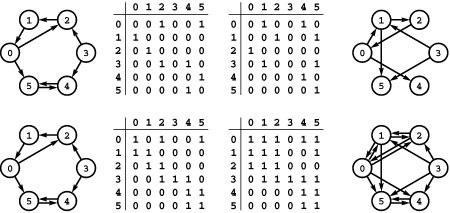
If we put 0s on the diagonal of a digraph’s adjacency matrix, the square of the matrix represents a graph with an edge corresponding to each path of length 2 (top). If we put 1s on the diagonal, the square of the matrix represents a graph with an edge corresponding to each path of length 1 or 2 (bottom).
Property 19.6 We can compute the transitive closure of a digraph by constructing the latter’s adjacency matrix A, adding self-loops for every vertex, and computing AV.
Proof: Continuing the argument in the previous paragraph, A 3 has an edge for every path of length less than or equal to 3 in the digraph, A 4 has an edge for every path of length less than or equal to 4 in the digraph, and so forth. We do not need to consider paths of length greater than V because of the pigeonhole principle: Any such path must revisit some vertex (since there are only V of them) and therefore adds no information to the transitive closure because the same two vertices are connected by a directed path of length less than V (which we could obtain by removing the cycle to the revisited vertex).
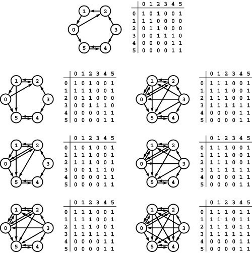
Figure 19.15 shows the adjacency-matrix powers for a sample digraph converging to transitive closure. This method takes V matrix multiplications, each of which takes time proportional to V3, for a grand total of V4. We can actually compute the transitive closure for any digraph with just lg [V] Boolean matrix-multiplication operations: We compute A 2, A 4, A 8,… until we reach an exponent greater than or equal to V. As shown in the proof of Property 19.6, A t = A V for any t > V; so the result of this computation, which requires time proportional to V3 lg V, is A V—the transitive closure.
Figure 19.15 Adjacency matrix powers and directed paths
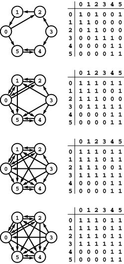
This sequence shows the first, second, third, and fourth powers (right, top to bottom) of the adjacency matrix at the top right, which gives graphs with edges for each of the paths of lengths less than 1, 2, 3, and 4, respectively, (left, top to bottom) in the graph that the matrix represents. The bottom graph is the transitive closure for this example, since there are no paths of length greater than 4 that connect vertices not connected by shorter paths.
Although the approach just described is appealing in its simplicity, an even simpler method is available. We can compute the transitive closure with just one operation of this kind, building up the transitive closure from the adjacency matrix in place, as follows:
for (i = 0; i < V;  i++)
  for (s = 0; s < V;  s++)
    for (t = 0; t < V;  t++)
      if (A[s][i] && A[i][t]) A[s][t] = 1;
This classical method, invented by S. Warshall in 1962, is the method of choice for computing the transitive closure of dense digraphs. The code is similar to the code that we might try to use to square a Boolean matrix in place: The difference (which is significant!) lies in the order of the for loops.
Property 19.7 With Warshall’s algorithm, we can compute the transitive closure of a digraph in time proportional to V3.
Proof: The running time is immediately evident from the structure of the code. We prove that it computes the transitive closure by induction on i. After the first iteration of the loop, the matrix has a 1 in row s and column t if and only if we have either the paths s-t or s-0-t. The second iteration checks all the paths between s and t that include 1 and perhaps 0, such as s-1-t, s-1-0-t, and s-0-1-t. We are led to the following inductive hypothesis: The ith iteration of the loop sets the bit in row s and column t in the matrix to 1 if and only if there is a directed path from s to t in the digraph that does not include any vertices with indices greater than i (except possibly the endpoints s and t). As just argued, the condition is true when i is 0, after the first iteration of the loop. Assuming that it is true for the ith iteration of the loop, there is a path from s to t that does not include any vertices with indices greater than i+1 if and only if ( i ) there is a path from s to t that does not include any vertices with indices greater than i, in which case A[s][t] was set on a previous iteration of the loop (by the inductive hypothesis); or ( ii ) there is a path from s to i+1 and a path from i+1 to t, neither of which includes any vertices with indices greater than i (except endpoints), in which case A[s][i+1] and A[i+1][t] were previously set to 1 (by hypothesis), so the inner loop sets A[s][t].
Figure 19.16 Warshall’s algorithm
This sequence shows the development of the transitive closure (bottom) of an example digraph (top) as computed with Warshall’s algorithm. The first iteration of the loop (left column, top) adds the edges 1-2 and 1-5 because of the paths 1-0-2 and 1-0-5, which include vertex 0 (but no vertex with a higher number); the second iteration of the loop (left column, second from top) adds the edges 2-0 and 2-5 because of the paths 2-1-0 and 2-1-0-5, which include vertex 1 (but no vertex with a higher number); and the third iteration of the loop (left column, bottom) adds the edges 0-1, 3-0, 3-1, and 3-5 because of the paths 0-2-1, 3-2-1-0, 3-2-1, and 3-2-1-0-5, which include vertex 2 (but no vertex with a higher number). The right column shows the edges added when paths through 3, 4, and 5 are considered. The last iteration of the loop (right column, bottom) adds the edges from 0, 1, and 2, to 4, because the only directed paths from those nodes to 4 include 5, the highest-numbered vertex.
We can improve the performance of Warshall’s algorithm with a simple transformation of the code: We move the test of A[s][i] out of the inner loop because its value does not change as t varies. This move allows us to avoid executing the t loop entirely when A[s][i] is zero. The savings that we achieve from this improvement depends on the digraph and is substantial for many digraphs (see Exercises 19.53 and 19.54). Program 19.3 implements this improvement and packages Warshall’s method such that clients can preprocess a digraph (compute the transitive closure), then compute the answer to any reachability query in constant time.
We are interested in pursuing more efficient solutions, particularly for sparse digraphs. We would like to reduce both the preprocessing time and the space because both make the use of Warshall’s method prohibitively costly for huge sparse digraphs.
In modern applications, abstract data types provide us with the ability to separate out the idea of an operation from any particular implementation so that we can focus on efficient implementations. For the transitive closure, this point of view leads to a recognition that we do not necessarily need to compute the entire matrix to provide clients with the transitive-closure abstraction. One possibility might be that the transitive closure is a huge sparse matrix, so an adjacency-lists representation is called for because we cannot store the matrix representation. Even when the transitive closure is dense, client programs might test only a tiny fraction of possible pairs of edges, so computing the whole matrix is wasteful.
We use the term abstract transitive closure to refer to an ADT that provides clients with the ability to test reachability after preprocessing a digraph, like Program 19.3. In this context, we need to measure an algorithm not just by its cost to compute the transitive closure (preprocessing cost) but also by the space required and the query time achieved. That is, we rephrase Property 19.7 as follows:
Property 19.8 We can support constant-time reachability testing (abstract transitive closure) for a digraph, using space proportional to V2 and time proportional to V3 for preprocessing.
This property follows immediately from the basic performance characteristics of Warshall’s algorithm.
For most applications, our goal is not just to compute the transitive closure of a digraph quickly but also to support constant query time for the abstract transitive closure using far less space and far less preprocessing time than specified in Property 19.8. Can we find an implementation that will allow us to build clients that can afford to handle such digraphs? We return to this question in Section 19.8.
There is an intimate relationship between the problem of computing the transitive closure of a digraph and a number of other fundamental computational problems, and that relationship can help us to understand this problem’s difficulty. We conclude this section by considering two examples of such problems.
First, we consider the relationship between the transitive closure and the all-pairs shortest-paths problem (see Section 18.7). For di-graphs, the problem is to find, for each pair of vertices, a directed path with a minimal number of edges.
Given a digraph, we initialize a V -by- V integer matrix A by setting A[s][t] to 1 if thereisanedgefrom s to t andtothe sentinel value V if there is no such edge. Our goal is to set A[s][t] equal to the length of (the number of edges on) a shortest directed path from s to t, using the sentinel value V to indicate that there is no such path. The following code accomplishes this objective:
for (i = 0; i < V; i++)
  for (s = 0; s < V;  s++)
    for (t = 0; t < V;  t++)
      if (A[s][i] + A[i][t] < A[s][t])
        A[s][t] = A[s][i] + A[i][t];
This code differs from the version of Warshall’s algorithm that we saw just before Property 19.7 in only the if statement in the inner loop. Indeed, in the proper abstract setting, the computations are precisely the same (see Exercises 19.55 and 19.56). Converting the proof of Property 19.7 into a direct proof that this method accomplishes the desired objective is straightforward. This method is a special case of Floyd’s algorithm for finding shortest paths in weighted graphs (see Chapter 21). The BFS-based solution for undirected graphs that we considered in Section 18.7 also finds shortest paths in digraphs (appropriately modified). Shortest paths are the subject of Chapter 21, so we defer considering detailed performance comparisons until then.
Second, as we have seen, the transitive-closure problem is also closely related to the Boolean matrix-multiplication problem. The basic algorithms that we have seen for both problems require time proportional to V3, using similar computational schema. Boolean matrix multiplication is known to be a difficult computational problem: Algorithms that are asymptotically faster than the straightforward method are known, but it is debatable whether the savings are sufficiently large to justify the effort of implementing any of them. This fact is signifi-cant in the present context because we could use a fast algorithm for Boolean matrix multiplication to develop a fast transitive-closure algorithm (slower by just a factor of lg V ) using the repeated-squaring method illustrated in Figure 19.15. Conversely, we have a lower bound on the difficulty of computing the transitive closure:
Property 19.9 We can use any transitive-closure algorithm to compute the product of two Boolean matrices with at most a constant-factor difference in running time.
Proof: Given two V -by- V Boolean matrices A and B, we construct the following 3 V -by-3 V matrix:
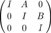
Here, 0 denotes the V -by- V matrix with all entries equal to 0, and I denotes the V -by- V identity matrix with all entries equal to 0 except those on the diagonal, which are equal to 1. Now, we consider this matrix to be the adjacency matrix for a digraph and compute its transitive closure by repeated squaring. But we only need one step:
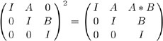
The matrix on the right-hand side of this equation is the transitive closure because further multiplications give back the same matrix. But this matrix has the V -by- V product A B in its upper-right corner. Whatever algorithm we use to solve the transitive-closure problem, we can use it to solve the Boolean matrix-multiplication problem at the same cost (to within a constant factor).
The significance of this property depends on the conviction of experts that Boolean matrix multiplication is difficult: Mathematicians have been working for decades to try to learn precisely how difficult it is, and the question is unresolved; the best known results say that the running time should be proportional to about V2 . 5 ( see reference section ). Now, if we could find a linear-time (proportional to V2) solution to the transitive-closure problem, then we would have a linear-time solution to the Boolean matrix-multiplication problem as well. This relationship between problems is known as reduction: We say that the Boolean matrix-multiplication problem reduces to the transitive-closure problem (see Section 21.6 and Part 8). Indeed, the proof actually shows that Boolean matrix multiplication reduces to finding the paths of length 2 in a digraph.
Despite a great deal of research by many people, no one has been able to find a linear-time Boolean matrix-multiplication algorithm, so we cannot present a simple linear-time transitive-closure algorithm. On the other hand, no one has proved that no such algorithm exists, so we hold open that possibility for the future. In short, we take Property 19.9 to mean that, barring a research breakthrough, we cannot expect the worst-case running time of any transitive-closure algorithm that we can concoct to be proportional to V2. Despite this conclusion, we can develop fast algorithms for certain classes of digraphs. For example, we have already touched on a simple method for computing the transitive closure that is much faster than Warshall’s algorithm for sparse digraphs.
Property 19.10 With DFS, we can support constant query time for the abstract transitive closure of a digraph, with space proportional to V2 and time proportional to V ( E + V ) for preprocessing (computing the transitive closure).
Proof: As we observed in the previous section, DFS gives us all the vertices reachable from the start vertex in time proportional to E, if we use the adjacency-lists representation (see Property 19.5 and Figure 19.11). Therefore, if we run DFS V times, once with each vertex as the start vertex, then we can compute the set of vertices reachable from each vertex—the transitive closure—in time proportional to V ( E + V ). The same argument holds for any linear-time generalized search (see Section 18.8 and Exercise 19.66).
Program 19.4 is an implementation of this search-based transitive-closure algorithm. This class implements the same interface as does Program 19.3. The result of running this program on the sample di-graph in Figure 19.1 is illustrated in the first tree in each forest in Figure 19.11.
For sparse digraphs, this search-based approach is the method of choice. For example, if E is proportional to V, then Program 19.4 computes the transitive closure in time proportional to V2. How can it do so, given the reduction to Boolean matrix multiplication that we just considered? The answer is that this transitive-closure algorithm does indeed give an optimal way to multiply certain types of Boolean matrices (those with O ( V ) nonzero entries). The lower bound tells us that we should not expect to find a transitive-closure algorithm that runs in time proportional to V2 for all digraphs, but it does not preclude the possibility that we might find algorithms, like this one, that are faster for certain classes of digraphs. If such graphs are the ones that we need to process, the relationship between transitive closure and Boolean matrix multiplication may not be relevant to us.
It is easy to extend the methods that we have described in this section to provide clients with the ability to find a specific path connecting two vertices by keeping track of the search tree, as described in Section 17.8. We consider specific ADT implementations of this sort in the context of the more general shortest-paths problems in Chapter 21.
Table 19.1 shows empirical results comparing the elementary transitive-closure algorithms described in this section. The adjacency-lists implementation of the search-based solution is by far the fastest method for sparse digraphs. The implementations all compute an adjacency matrix (of size V2), so none of them are suitable for huge sparse digraphs.
Table 19.1 Empirical study of transitive-closure algorithms
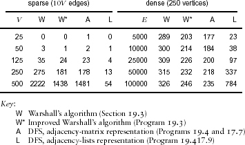
This table shows running times that exhibit dramatic performance differences for various algorithms for computing the transitive closure of random digraphs, both dense and sparse. For all but the adjacency-lists DFS, the running time goes up by a factor of 8 when we double V, which supports the conclusion that it is essentially proportional to V3. The adjacency-lists DFS takes time proportional to V E, which explains the running time roughly increasing by a factor of 4 when we double both V and E (sparse graphs) and by a factor of about 2 when we double E (dense graphs), except that list-traversal overhead degrades performance for high-density graphs.
For sparse digraphs whose transitive closure is also sparse, we might use an adjacency-lists implementation for the closure so that the size of the output is proportional to the number of edges in the transitive closure. This number certainly is a lower bound on the cost of computing the transitive closure, which we can achieve for certain types of digraphs using various algorithmic techniques (see Exercises 19.64 and 19.65). Despite this possibility, we generally view the objective of a transitive-closure computation to be dense, so we can use a representation like DenseGRAPH that can easily answer reachability queries, and we regard transitive-closure algorithms that compute the matrix in time proportional to V2 as being optimal since they take time proportional to the size of their output.
If the adjacency matrix is symmetric, it is equivalent to an undirected graph, and finding the transitive closure is the same as finding the connected components—the transitive closure is the union of complete graphs on the vertices in the connected components (see Exercise 19.48). Our connectivity algorithms in Section 18.5 amount to an abstract–transitive-closure computation for symmetric digraphs (undirected graphs) that uses space proportional to V and still supports constant-time reachability queries. Can we do as well in general digraphs? Can we reduce the preprocessing time still further? For what types of graphs can we compute the transitive closure in linear time? To answer these questions, we need to study the structure of digraphs in more detail, including, specifically, that of DAGs.
Exercises
• 19.46 What is the transitive closure of a digraph that consists solely of a directed cycle with V vertices?
19.47 How many edges are there in the transitive closure of a digraph that consists solely of a simple directed path with V vertices?
• 19.48 Give the transitive closure of the undirected graph
3-7 1-4 7-8 0-5 5-2 3-8 2-9 0-6 4-9 2-6 6-4.
• 19.49 Show how to construct a digraph with V vertices and E edges with the property that the number of edges in the transitive closure is proportional to t, for any t between E and V2. As usual, assume that E > V.
19.50 Give a formula for the number of edges in the transitive closure of a digraph that is a directed forest as a function of structural properties of the forest.
19.51 Show, in the style of Figure 19.15, the process of computing the transitive closure of the digraph
3-7 1-4 7-8 0-5 5-2 3-8 2-9 0-6 4-9 2-6 6-4
through repeated squaring.
19.52 Show, in the style of Figure 19.16, the process of computing the transitive closure of the digraph
3-7 1-4 7-8 0-5 5-2 3-8 2-9 0-6 4-9 2-6 6-4
with Warshall’s algorithm.
• 19.53 Give a family of sparse digraphs for which the improved version of Warshall’s algorithm for computing the transitive closure (Program 19.3) runs in time proportional to V E.
• 19.54 Find a sparse digraph for which the improved version of Warshall’s algorithm for computing the transitive closure (Program 19.3) runs in time proportional to V3.
• 19.55 Develop a base class from which you can derive classes that implement both Warshall’s algorithm and Floyd’s algorithm. (This exercise is a version of Exercise 19.56 for people who are more familiar with abstract data types than with abstract algebra.)
• 19.56 Use abstract algebra to develop a generic algorithm that encompasses both Warshall’s algorithm and Floyd’s algorithm. (This exercise is a version of Exercise 19.55 for people who are more familiar with abstract algebra than with abstract data types.)
• 19.57 Show, in the style of Figure 19.16, the development of the all-shortest paths matrix for the example graph in the figure as computed with Floyd’s algorithm.
19.58 Is the Boolean product of two symmetric matrices symmetric? Explain your answer.
19.59 Add a public function member to Programs 19.3 and 19.4 to allow clients to use tc objects to find the number of edges in the transitive closure.
19.60 Design a way to maintain the count of the number of edges in the transitive closure by modifying it when edges are added and removed. Give the cost of adding and removing edges with your scheme.
• 19.61 Add a public member function for use with Programs 19.3 and 19.4 that returns a vertex-indexed vector that indicates which vertices are reachable from a given vertex.
• 19.62 Run empirical studies to determine the number of edges in the transitive closure, for various types of digraphs (see Exercises 19.11–18).
• 19.63 Consider the bit-matrix graph representation that is described in Exercise 17.23. Which method can you speed up by a factor of B (where B is the number of bits per word on your computer): Warshall’s algorithm or the DFS-based algorithm? Justify your answer by developing an implementation that does so.
• 19.64 Give a program that computes the transitive closure of a digraph that is a directed forest in time proportional to the number of edges in the transitive closure.
• 19.65 Implement an abstract–transitive-closure algorithm for sparse graphs that uses space proportional to T and can answer reachability requests in constant time after preprocessing time proportional to V E + T, where T is the number of edges in the transitive closure. Hint: Use dynamic hashing.
• 19.66 Provide a version of Program 19.4 that is based on generalized graph search (see Section 18.8), and run empirical studies to see whether the choice of graph-search algorithm has any effect on performance.
19.4 Equivalence Relations and Partial Orders
This section is concerned with basic concepts in set theory and their relationship to abstract–transitive-closure algorithms. Its purposes are to put the ideas that we are studying into a larger context and to demonstrate the wide applicability of the algorithms that we are considering. Mathematically inclined readers who are familiar with set theory may wish to skip to Section 19.5 because the material that we cover is elementary (although our brief review of terminology may be helpful); readers who are not familiar with set theory may wish to consult an elementary text on discrete mathematics because our treatment is rather succinct. The connections between digraphs and these fundamental mathematical concepts are too important for us to ignore.
Given a set, a relation among its objects is defined to be a set of ordered pairs of the objects. Except possibly for details relating to parallel edges and self-loops, this definition is the same as our definition of a digraph: Relations and digraphs are different representations of the same abstraction. The mathematical concept is somewhat more powerful because the sets may be infinite, whereas our computer programs all work with finite sets, but we ignore this difference for the moment.
Typically, we choose a symbol R and use the notation sRt as shorthand for the statement “the ordered pair ( s, t ) is in the relation R.” For example, we use the symbol “<” to represent the “less than” relation among numbers. Using this terminology, we can characterize various properties of relations. For example, a relation R is said to be symmetric if sRt implies that tRs for all s and t;itissaidtobe reflexive if sRs for all s. Symmetric relations are the same as undirected graphs. Reflexive relations correspond to graphs in which all vertices have self-loops; relations that correspond to graphs where no vertices have self-loops are said to be irreflexive.
A relation R is said to be transitive when sRt and tRu implies that sRu for all s, t, and u. The transitive closure of a relation is a well-defined concept; but instead of redefining it in set-theoretic terms, we appeal to the definition that we gave for digraphs in Section 19.3. Any relation is equivalent to a digraph, and the transitive closure of the relation is equivalent to the transitive closure of the digraph. The transitive closure of any relation is transitive.
In the context of graph algorithms, we are particularly interested in two particular transitive relations that are defined by further constraints. These two types, which are widely applicable, are known as equivalence relations and partial orders.
An equivalence relation is a transitive relation that is also reflexive and symmetric. Note that a symmetric, transitive relation that includes each object in some ordered pair must be an equivalence relation: If s t, then t s (by symmetry) and s s (by transitivity). Equivalence relations divide the objects in a set into subsets known as equivalence classes. Two objects s and t are in the same equivalence class if and only if s t. The following examples are typical equivalence relations:
Modular arithmetic Any positive integer k defines an equivalence relation on the set of integers, with s t (mod k ) if and only if the remainder that results when we divide s by k is equal to the the remainder that results when we divide t by k. The relation is obviously symmetric; a short proof establishes that it is also transitive (see Exercise 19.67) and therefore is an equivalence relation.
Connectivity in graphs The relation “is in the same connected component as” among vertices is an equivalence relation because it is symmetric and transitive. The equivalence classes correspond to the connected components in the graph.
When we build a graph ADT that gives clients the ability to test whether two vertices are in the same connected component, we are implementing an equivalence-relation ADT that provides clients with the ability to test whether two objects are equivalent. In practice, this correspondence is significant because the graph is a succinct representation of the equivalence relation (see Exercise 19.71). In fact, as we saw in Chapters 1 and 18, to build such an ADT we need to maintain only a single vertex-indexed vector.
A partial order ![]() is a transitive relation that is also irreflexive. As a direct consequence of transitivity and irreflexivity, it is trivial to prove that partial orders are also asymmetric: If s
is a transitive relation that is also irreflexive. As a direct consequence of transitivity and irreflexivity, it is trivial to prove that partial orders are also asymmetric: If s ![]() t and t
t and t ![]() s, then s
s, then s ![]() s (by transitivity), which contradicts irreflexivity, so we cannot have both s
s (by transitivity), which contradicts irreflexivity, so we cannot have both s ![]() t and t
t and t ![]() s. Moreover, extending the same argument shows that a partial order cannot have a cycle, such as s
s. Moreover, extending the same argument shows that a partial order cannot have a cycle, such as s ![]() t, t
t, t ![]() u, and u
u, and u ![]() s. The following examples are typical partial orders:
s. The following examples are typical partial orders:
Subset inclusion The relation “includes but is not equal to” (⊂) among subsets of a given set is a partial order—it is certainly irreflexive, and if s ⊂ t and t ⊂ u, then certainly s ⊂ u.
Paths in DAGs The relation “can be reached by a nonempty directed path from” is a partial order on vertices in DAGs with no self-loops because it is transitive and irreflexive. Like equivalence relations and undirected graphs, this particular partial order is significant for many applications because a DAG provides a succinct implicit representation of the partial order. For example, Figure 19.17 illustrates DAGs for subset containment partial orders whose number of edges is only a fraction of the cardinality of the partial order (see Exercise 19.73).
Figure 19.17 Set-inclusion DAG
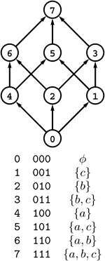
In the DAG at the top, we interpret vertex indices to represent subsets of a set of 3 elements, as shown in the table at the bottom. The transitive closure of this DAG represents the subset inclusion partial order: There is a directed path between two nodes if and only if the subset represented by the first is included in the subset represented by the second.
Indeed, we rarely define partial orders by enumerating all their ordered pairs, because there are too many of such pairs. Instead, we generally specify an irreflexive relation (a DAG) and consider its transitive closure. This usage is a primary reason for considering abstract–transitive-closure ADT implementations for DAGs. Using DAGs, we consider examples of partial orders in Section 19.5.
A total order T is a partial order where either sT t or tT s for all s [negationslash] = t. Familiar examples of total orders are the “less than” relation among integers or real numbers and lexicographic ordering among strings of characters. Our study of sorting and searching algorithms in Parts 3 and 4 was based on a total-order ADT implementation for sets. In a total order, there is one and only one way to arrange the elements in the set such that sT t whenever s is before t in the arrangement; in a partial order that is not total, there are many ways to do so. In Section 19.5, we examine algorithms for this task.
In summary, the following correspondences between sets and graph models help us to understand the importance and wide applicability of fundamental graph algorithms.
• Relations and digraphs
• Symmetric relations and undirected graphs
• Transitive relations and paths in graphs
• Equivalence relations and paths in undirected graphs
• Partial orders and paths in DAGs
This context places in perspective the types of graphs and algorithms that we are considering and provides one motivation for us to move on to consider basic properties of DAGs and algorithms for processing those DAGs.
Exercises
19.67 Show that “has the same remainder after dividing by k” is a transitive relation (and therefore is an equivalence relation) on the set of integers.
19.68 Show that “is in the same edge-connected component as” is an equivalence relation among vertices in any graph.
19.69 Show that “is in the same biconnected component as” is not an equivalence relation among vertices in all graphs.
19.70 Prove that the transitive closure of an equivalence relation is an equivalence relation and that the transitive closure of a partial order is a partial order.
• 19.71 The cardinality of a relation is its number of ordered pairs. Prove that the cardinality of an equivalence relation is equal to the sum of the squares of the cardinalities of that relation’s equivalence classes.
• 19.72 Using an online dictionary, build a graph that represents the equivalence relation “has k letters in common with” among words. Determine the number of equivalence classes for k =1 through 5.
19.73 The cardinality of a partial order is its number of ordered pairs. What is the cardinality of the subset containment partial order for an n -element set?
• 19.74 Show that “is a factor of” is a partial order among integers.
19.5 DAGs
In this section, we consider various applications of directed acyclic graphs (DAGs). We have two reasons to do so. First, because they serve as implicit models for partial orders, we work directly with DAGs in many applications and need efficient algorithms to process them. Second, these various applications give us insight into the nature of DAGs, and understanding DAGs is essential to understanding general digraphs.
Since DAGs are a special type of digraph, all DAG-processing problems trivially reduce to digraph-processing problems. Although we expect processing DAGs to be easier than processing general di-graphs, we know when we encounter a problem that is difficult to solve on DAGs we should not expect to do any better solving the same problem on general digraphs. As we shall see, the problem of computing the transitive closure lies in this category. Conversely, understanding the difficulty of processing DAGs is important because every digraph has a kernel DAG (see Property 19.2), so we encounter DAGs even when we work with digraphs that are not DAGs.
The prototypical application where DAGs arise directly is called scheduling. Generally, solving scheduling problems has to do with arranging for the completion of a set of tasks, under a set of constraints, by specifying when and how the tasks are to be performed. Constraints might involve functions of the time taken or other resources consumed by the tasks. The most important type of constraints are precedence constraints, which specify that certain tasks must be performed before certain others, thus comprising a partial order among the tasks. Different types of additional constraints lead to many different types of scheduling problems, of varying difficulty. Literally thousands of different problems have been studied, and researchers still seek better algorithms for many of them. Perhaps the simplest nontrivial scheduling problem may be stated as follows:
Scheduling Given a set of tasks to be completed, with a partial order that specifies that certain tasks have to be completed before certain other tasks are begun, how can we schedule the tasks such that they are all completed while still respecting the partial order?
In this basic form, the scheduling problem is called topological sorting; it is not difficult to solve, as we shall see in the next section by examining two algorithms that do so. In more complicated practical applications, we might need to add other constraints on how the tasks might be scheduled, and the problem can become much more difficult. For example, the tasks might correspond to courses in a student’s schedule, with the partial order specifying prerequisites. Topological sorting gives a feasible course schedule that meets the prerequisite requirements, but perhaps not one that respects other constraints that need to be added to the model, such as course conflicts, limitations on enrollments, and so forth. As another example, the tasks might be part of a manufacturing process, with the partial order specifying sequential requirements of the particular process. Topological sorting gives us a way to schedule the tasks, but perhaps there is another way to do so that uses less time, money, or some other resources not included in the model. We examine versions of the scheduling problem that capture more general situations such as these in Chapters 21 and 22.
Often, our first task is to check whether or not a given DAG indeed has no directed cycles. As we saw in Section 19.2, we can easily implement a class that allows clients to test whether a general digraph is a DAG in linear time, by running a standard DFS and checking that the DFS forest has no back edges (see Exercise 19.75). To implement DAG-specific algorithms, we implement task-specific client classes of our standard GRAPH ADT that assume they are processing digraphs with no cycles, leaving the client the responsibility of checking for cycles. This arrangement allows for the possibility that a DAG-processing algorithm produces useful results even when run on a digraph with cycles, which is sometimes the case. Sections 19.6 and 19.7 are devoted to implementations of classes for topological sorting (DAGts) and reachability in DAGs (DAGtc and DAGreach); Program 19.13 is an example of a client of such a class.
In a sense, DAGs are part tree, part graph. We can certainly take advantage of their special structure when we process them. For example, we can view a DAG almost as we view a tree, if we wish. Suppose that we want to traverse the vertices of the DAG D as though it were a tree rooted at w, so that, for example, the result of traversing the two DAGs in Figure 19.18 with this program would be the same. The following simple program accomplishes this task in the same manner as would a recursive tree traversal:
void traverseR(Dag D, int v)
 {
   visit(v);
   typename Dag::adjIterator A(D, v);
    for (int t = A.beg(); !A.end(); t = A.nxt())
     traverseR(D, t);
 }
We rarely use a full traversal of this kind, however, because we normally want to take advantage of the same economies that save space in a DAG to save time in traversing it (for example, by marking visited nodes in a normal DFS). The same idea applies to a search, where we make a recursive call for only one link incident on each vertex. In such an algorithm, the search cost will be the same for the DAG and the tree, but the DAG uses far less space.
Because they provide a compact way to represent trees that have identical subtrees, we often use DAGs instead of trees when we represent computational abstractions. In the context of algorithm design, the distinction between the DAG representation and the tree representation of a program in execution is the essential distinction behind dynamic programming (see, for example, Figure 19.18 and Exercise 19.78). DAGs are also widely used in compilers as intermediate representations of arithmetic expressions and programs (see, for example, Figure 19.19) and in circuit-design systems as intermediate representations of combinational circuits.
Along these lines, an important example that has many applications arises when we consider binary trees. We can apply the same restriction to DAGs that we applied to trees to define binary trees.
Definition 19.6 A binary DAG is a directed acyclic graph with two edges leaving each node, identified as the left edge and the right edge, either or both of which may be null.
Figure 19.18 DAG model of Fibonacci computation
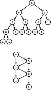
The tree at the top shows the dependence of computing each Fibonacci number on computing its two predecessors. The DAG at the bottom shows the same dependence with only a fraction of the nodes.
The distinction between a binary DAG and a binary tree is that in the binary DAG we can have more than one link pointing to a node. As did our definition for binary trees, this definition models a natural representation, where each node is a structure with a left link and a right link that point to other nodes (or are null), subject to only the global restriction that no directed cycles are allowed. Binary DAGs are significant because they provide a compact way to represent binary trees in certain applications. For example, we can compress an existence trie into a binary DAG without changing the search implementation, as shown Figure 19.20 and Program 19.5.
Figure 19.19 DAG representation of an arithmetic expression
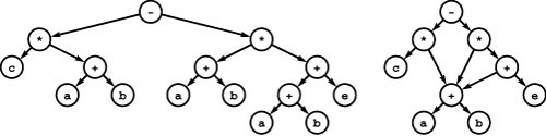
Both of these DAGs are representations of the arithmetic expression (c*(a+b))-((a+b))*((a+b)+e)). In the binary parse tree at left, leaf nodes represent operands and internal nodes each represent operators to be applied to the expressions represented by their two subtrees (see Figure 5.31). The DAG at right is a more compact representation of the same tree. More important, we can compute the value of the expression in time proportional to the size of the DAG, which is typically significantly less than the size of the tree (see Exercises 19.112 and 19.113).
An equivalent application is to view the trie keys as corresponding to rows in the truth table of a Boolean function for which the function is true (see Exercises 19.84 through 19.87). The binary DAG is a model for an economical circuit that computes the function. In this application, binary DAGs are known as binary decision diagrams (BDD) s.
Motivated by these applications, we turn, in the next two sections, to the study of DAG-processing algorithms. Not only do these algorithms lead to efficient and useful DAG ADT function implementations, but also they provide insight into the difficulty of processing digraphs. As we shall see, even though DAGs would seem to be substantially simpler structures than general digraphs, some basic problems are apparently no easier to solve.
Exercises
• 19.75 Implement a DFS class for use by clients for verifying that a DAG has no cycles.
• 19.76 Write a program that generates random DAGs by generating random digraphs, doing a DFS from a random starting point, and throwing out the back edges (see Exercise 19.40). Run experiments to decide how to set parameters in your program to expect DAGs with E edges, given V.
• 19.77 How many nodes are there in the tree and in the DAG corresponding to Figure 19.18 for FN, the Nth Fibonacci number?
19.78 Give the DAG corresponding to the dynamic-programming example for the knapsack model from Chapter 5 (see Figure 5.17).
• 19.79 Develop an ADT for binary DAGs.
Figure 19.20 Binary tree compression
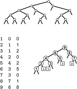
The table of nine pairs of integers at the bottom left is a compact representation of a binary DAG (bottom right) that is a compressed version of the binary tree structure at top. Node labels are not explicitly stored in the data structure: The table represents the eighteen edges 1-0, 1-0, 2-1, 2-1, 3-1, 3-2, and so forth, but designates a left edge and a right edge leaving each node (as in a binary tree) and leaves the source vertex for each edge implicit in the table index.
An algorithm that depends only upon the tree shape will work effectively on the DAG. For example, suppose that the tree is an existence trie for binary keys corresponding to the leaf nodes, so it represents the keys 0000, 0001, 0010, 0110, 1100, and 1101. A successful search for the key 1101 in the trie moves right, right, left, and right to end at a leaf node. In the DAG, the same search goes from 9 to 8 to 7 to 2 to 1.
• 19.80 Can every DAG be represented as a binary DAG (see Property 5.4)?
• 19.81 Write a function that performs an inorder traversal of a single-source binary DAG. That is, the function should visit all vertices that can be reached via the left edge, then visit the source, then visit all the vertices that can be reached via the right edge.
• 19.82 In the style of Figure 19.20, give the existence trie and corresponding binary DAG for the keys 01001010 10010101 00100001 11101100 01010001 00100001 00000111 01010011.
19.83 Implement an ADT based on building an existence trie from a set of 32-bit keys, compressing it as a binary DAG, then using that data structure to support existence queries.
• 19.84 Draw the BDD for the truth table for the odd parity function of four variables, which is 1 if and only if the number of variables that have the value 1 is odd.
19.85 Write a function that takes a 2n-bit truth table as argument and returns the corresponding BDD. For example, given the input 1110001000001100, your program should return a representation of the binary DAG in Figure 19.20.
19.86 Write a function that takes a 2n-bit truth table as argument, computes every permutation of its argument variables, and, using your solution to Exercise 19.85, finds the permutation that leads to the smallest BDD.
• 19.87 Run empirical studies to determine the effectiveness of the strategy of Exercise 19.87 for various Boolean functions, both standard and randomly generated.
19.88 Write a program like Program 19.5 that supports common subexpression removal: Given a binary tree that represents an arithmetic expression, compute a binary DAG that represents the same expression with common subexpressions removed.
• 19.89 Draw all the nonisomorphic DAGs with two, three, four, and five vertices.
••19.90 How many different DAGs are there with V vertices and E edges?
••• 19.91 How many different DAGs are there with V vertices and E edges, if we consider two DAGs to be different only if they are not isomorphic?
Figure 19.21 Topological sort (relabeling)
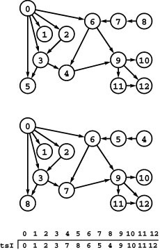
Given any DAG (top), topological sorting allows us to relabel its vertices so that every edge points from a lower-numbered vertex to a higher-numbered one (bottom). In this example, we relabel 4, 5, 7, and 8 to 7, 8, 5, and 4, respectively, as indicated in the array tsI. There are many possible labelings that achieve the desired result.
19.6 Topological Sorting
The goal of topological sorting is to be able to process the vertices of a DAG such that every vertex is processed before all the vertices to which it points. There are two natural ways to define this basic operation; they are essentially equivalent. Both tasks call for a permutation of the integers 0 through V-1, which we put in vertex-indexed vectors, as usual.
Topological sort (relabel) Given a DAG, relabel its vertices such that every directed edge points from a lower-numbered vertex to a higher-numbered one (see Figure 19.21).
Topological sort (rearrange) Given a DAG, rearrange its vertices on a horizontal line such that all the directed edges point from left to right (see Figure 19.22).
As indicated in Figure 19.22, it is easy to establish that the relabeling and rearrangement permutations are inverses of one another: Given a rearrangement, we can obtain a relabeling by assigning the label 0 to the first vertex on the list, 1 to the second label on the list, and so forth. For example, if a vector ts has the vertices in topologically sorted order, then the loop
Figure 19.22 Topological sorting (rearrangement)
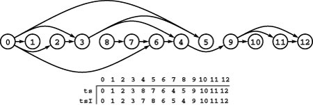
This diagram shows another way to look at the topological sort in Figure 19.21, where we specify a way to rearrange the vertices, rather than relabel them. When we place the vertices in the order specified in the array ts, from left to right, then all directed edges point from left to right. The inverse of the permutation ts is the permutation tsI that specifies the relabeling described in Figure 19.21.
for (i=0;i<V; i++) tsI[ts[i]] = i;
defines a relabeling in the vertex-indexed vector tsI. Conversely, we can get the rearrangement from the relabeling with the loop
for (i=0;i<V; i++) ts[tsI[i]] = i;
which puts the vertex that would have label 0 first in the list, the vertex that would have label 1 second in the list, and so forth. Most often, we use the term topological sort to refer to the rearrangement version of the problem. Note that ts is not a vertex-indexed vector.
In general, the vertex order produced by a topological sort is not unique. For example,
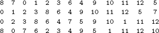
are all topological sorts of the example DAG in Figure 19.6 (and there are many others). In a scheduling application, this situation arises whenever one task has no direct or indirect dependence on another and thus they can be performed either before or after the other (or even in parallel). The number of possible schedules grows exponentially with the number of such pairs of tasks.
As we have noted, it is sometimes useful to interpret the edges in a digraph the other way around: We say that an edge directed from s to t means that vertex s “depends” on vertex t. For example, the vertices might represent terms to be defined in a book, with an edge from s to t if the definition of s uses t. In this case, it would be useful to find an ordering with the property that every term is defined before it is used in another definition. Using this ordering corresponds to positioning the vertices in a line such that edges all go from right to left—a reverse topological sort. Figure 19.23 illustrates a reverse topological sort of our sample DAG.
Figure 19.23 Reverse topological sort
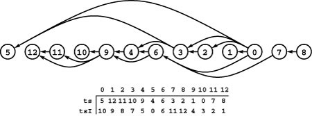
In this reverse topological sort of our sample digraph, the edges all point from right to left. Numbering the vertices as specified by the inverse permutation tsI gives a graph where every edge points from a higher-numbered vertex to a lower-numbered vertex.
Now, it turns out that we have already seen an algorithm for reverse topological sorting: our standard recursive DFS! When the input graph is a DAG, a postorder numbering puts the vertices in reverse topological order. That is, we number each vertex as the final action of the recursive DFS function, as in the post vector in the DFS implementation in Program 19.2. As illustrated in Figure 19.24, using this numbering is equivalent to numbering the nodes in the DFS forest in postorder, and gives a topological sort: The vertex-indexed vector post gives the relabeling and its inverse the rearrangement depicted in Figure 19.23—a reverse topological sort of the DAG.
Property 19.11 Postorder numbering in DFS yields a reverse topological sort for any DAG.
Proof: Suppose that s and t are two vertices such that s appears before t in the postorder numbering even though there is a directed edge s-t in the graph. Since we are finished with the recursive DFS for s at the time that we assign s its number, we have examined, in particular, the edge s-t. But if s-t were a tree, down, or cross edge, the recursive DFS for t would be complete, and t would have a lower number; however, s-t cannot be a back edge because that would imply a cycle. This contradiction implies that such an edge s-t cannot exist.
Thus, we can easily adapt a standard DFS to do a topological sort, as shown in Program 19.6. This implementation does a reverse topological sort: It computes the postorder numbering permutation and its inverse, so that clients can relabel or rearrange vertices.
Program 19.6 Reverse topological sort
This DFS class computes postorder numbering of the DFS forest (a reverse topological sort). Clients can use a TS object to relabel a DAG’s vertices so that every edge points from a higher-numbered vertex to a lower-numbered one or to arrange vertices such that the source vertex of every edge appears after the destination vertex (see Figure 19.23).
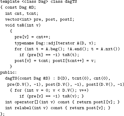
Figure 19.24 DFS forest for a DAG
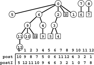
A DFS forest of a digraph has no back edges (edges to nodes with a higher postorder number) if and only if the digraph is a DAG. The non-tree edges in this DFS forest for the DAG of Figure 19.21 are either down edges (shaded squares) or cross edges (unshaded squares). The order in which vertices are encountered in a postorder walk of the forest, shown at the bottom, is a reverse topological sort (see Figure 19.23).
Computationally, the distinction between topological sort and reverse topological sort is not crucial. We can simply change the [] operator to return postI[G.V()-1 - v], or we can modify the implementation in one of the following ways:
• Do a reverse topological sort on the reverse of the given DAG.
• Rather than using it as an index for postorder numbering, push the vertex number on a stack as the final act of the recursive
procedure. After the search is complete, pop the vertices from the stack. They come off the stack in topological order.
• Number the vertices in reverse order (start at V 1 and count down to 0). If desired, compute the inverse of the vertex numbering to get the topological order.
The proofs that these changes give a proper topological ordering are left for you to do as an exercise (see Exercise 19.97).
To implement the first of the options listed in the previous paragraph for sparse graphs (represented with adjacency lists), we would need to use Program 19.1 to compute the reverse graph. Doing so essentially doubles our space usage, which may thus become onerous for huge graphs. For dense graphs (represented with an adjacency matrix), as noted in Section 19.1, we can do DFS on the reverse without using any extra space or doing any extra work, simply by exchanging rows and columns when referring to the matrix, as illustrated in Program 19.7.
Next, we consider an alternative classical method for topological sorting that is more like breadth-first search (BFS) (see Section 18.7). It is based on the following property of DAGs.
Property 19.12 Every DAG has at least one source and at least one sink.
Figure 19.25 Topologically sorting a DAG by removing sources
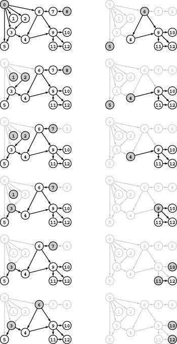
Since it is a source (no edges point to it), 0 can appear first in a topological sort of this example graph (left, top). If we remove 0 (and all the edges that point from it to other vertices), then 1 and 2 become sources in the resulting DAG (left, second from top), which we can then sort using the same algorithm. This figure illustrates the operation of Program 19.8, which picks from among the sources (the shaded nodes in each diagram) using the FIFO discipline, though any of the sources could be chosen at each step. See Figure 19.26 for the contents of the data structures that control the specific choices that the algorithm makes. The result of the topological sort illustrated here is the node order 082 1736 54 9111012.
Proof: Suppose that we have a DAG that has no sinks. Then, starting at any vertex, we can build an arbitrarily long directed path by following any edge from that vertex to any other vertex (there is at least one edge, since there are no sinks), then following another edge from that vertex, and so on. But once we have been to V +1 vertices, we must have seen a directed cycle, by the pigeonhole principle (see Property 19.6), which contradicts the assumption that we have a DAG. Therefore, every DAG has at least one sink. It follows that every DAG also has at least one source: its reverse’s sink.
From this fact, we can derive a topological-sort algorithm: Label any source with the smallest unused label, then remove it and label the rest of the DAG, using the same algorithm. Figure 19.25 is a trace of this algorithm in operation for our sample DAG.
Implementing this algorithm efficiently is a classic exercise in data-structure design ( see reference section ). First, there may be multiple sources, so we need to maintain a queue to keep track of them (any generalized queue will do). Second, we need to identify the sources in the DAG that remains when we remove a source. We can accomplish this task by maintaining a vertex-indexed vector that keeps track of the indegree of each vertex. Vertices with indegree 0 are sources, so we can initialize the queue with one scan through the DAG (using DFS or any other method that examines all of the edges). Then, we perform the following operations until the source queue is empty:
• Remove a source from the queue and label it.
• Decrement the entries in the indegree vector corresponding to the destination vertex of each of the removed vertex’s edges.
• If decrementing any entry causes it to become 0, insert the corresponding vertex onto the source queue.
Program 19.8 is an implementation of this method, using a FIFO queue, and Figure 19.26 illustrates its operation on our sample DAG, providing the details behind the dynamics of the example in Figure 19.25.
Figure 19.26 Indegree table and queue contents
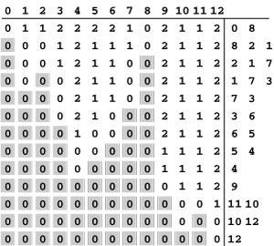
This sequence depicts the contents of the indegree table (left) and the source queue (right) during the execution of Program 19.8 on the sample DAG corresponding to Figure 19.25. At any given point in time, the source queue contains the nodes with indegree 0. Reading from top to bottom, we remove the leftmost node from the source queue, decrement the indegree entry corresponding to every edge leaving that node, and add any vertices whose entries become 0 to the source queue. For example, the second line of the table reflects the result of removing 0 from the source queue, then (because the DAG has the edges 0-1, 0-2, 0-3, 0-5, and 0-6) decrementing the indegree entries corresponding to 1, 2, 3, 5, and 6 and adding 2 and 1 to the source queue (because decrementing made their indegree entries 0). Reading the leftmost entries in the source queue from top to bottom gives a topological ordering for the graph.
The source queue does not empty until every vertex in the DAG is labeled, because the subgraph induced by the vertices not yet labeled is always a DAG, and every DAG has at least one source. Indeed, we can use the algorithm to test whether a graph is a DAG by inferring that there must be a cycle in the subgraph induced by the vertices not
Program 19.8 Source-queue–based topological sort
This class implements the same interface as does Programs 19.6 and 19.7. It maintains a queue of sources and uses a table that keeps track of the indegree of each vertex in the DAG induced by the vertices that have not been removed from the queue.
When we remove a source from the queue, we decrement the indegree entries corresponding to each of the vertices on its adjacency list (and put on the queue any vertices corresponding to entries that become 0). Vertices come off the queue in topologically sorted order.
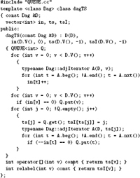
yet labeled if the queue empties before all the vertices are labeled (see Exercise 19.104).
Processing vertices in topologically sorted order is a basic technique in processing DAGs. A classic example is the problem of finding the length of the longest path in a DAG. Considering the vertices in reverse topologically sorted order, the length of the longest path originating at each vertex v is easy to compute: Add one to the maximum of the lengths of the longest paths originating at each of the vertices reachable by a single edge from v. The topological sort ensures that all those lengths are known when v is processed, and that no other paths from v will be found afterwards. For example, taking a left-to-right scan of the reverse topological sort shown in Figure 19.23, we can quickly compute the following table of lengths of the longest paths originating at each vertex in the sample graph in Figure 19.21.
For example, the 6 corresponding to 0 (third column from the right) says that there is a path of length 6 originating at 0, which we know because there is an edge 0-2, we previously found the length of the longest path from 2 to be 5, and no other edge from 0 leads to a node having a longer path.
Whenever we use topological sorting for such an application, we have several choices in developing an implementation:
• Use DAGts in a DAG ADT, then proceed through the vector it computes to process the vertices.
• Process the vertices after the recursive calls in a DFS.
• Process the vertices as they come off the queue in a source-queue– based topological sort.
All of these methods are used in DAG-processing implementations in the literature, and it is important to know that they are all equivalent. We will consider other topological-sort applications in Exercises 19.111 and 19.114 and in Sections 19.7 and 21.4.
Exercises
• 19.92 Write a function that checks whether or not a given permutation of a DAG’s vertices is a proper topological sort of that DAG.
19.93 How many different topological sorts are there of the DAG that is depicted in Figure 19.6?
• 19.94 Give the DFS forest and the reverse topological sort that results from doing a standard adjacency-lists DFS (with postorder numbering) of the DAG
3-7 1-4 7-8 0-5 5-2 3-8 2-9 0-6 4-9 2-6 6-4 4-3 2-3.
• 19.95 Give the DFS forest and the topological sort that results from building a standard adjacency-lists representation of the DAG
3-7 1-4 7-8 0-5 5-2 3-8 2-9 0-6 4-9 2-6 6-4 4-3 2-3,
then using Program 19.1 to build the reverse, then doing a standard adjacency-lists DFS with postorder numbering.
• 19.96 Program 19.6 uses postorder numbering to do a reverse topological sort—why not use preorder numbering to do a topological sort? Give a three-vertex example that illustrates the reason.
• 19.97 Prove the correctness of each of the three suggestions given in the text for modifying DFS with postorder numbering such that it computes a topological sort instead of a reverse topological sort.
• 19.98 Give the DFS forest and the topological sort that results from doing a standard adjacency-matrix DFS with implicit reversal (and postorder numbering) of the DAG
3-7 1-4 7-8 0-5 5-2 3-8 2-9 0-6 4-9 2-6 6-4 4-3 2-3
(see Program 19.7).
• 19.99 Given a DAG, does there exist a topological sort that cannot result from applying a DFS-based algorithm, no matter what order the vertices adjacent to each vertex are chosen? Prove your answer.
• 19.100 Show, in the style of Figure 19.26, the process of topologically sorting the DAG
3-7 1-4 7-8 0-5 5-2 3-8 2-9 0-6 4-9 2-6 6-4 4-3 2-3
with the source-queue algorithm (Program 19.8).
• 19.101 Give the topological sort that results if the data structure used in the example depicted in Figure 19.25 is a stack rather than a queue.
• 19.102 Given a DAG, does there exist a topological sort that cannot result from applying the source-queue algorithm, no matter what queue discipline is used? Prove your answer.
19.103 Modify the source-queue topological-sort algorithm to use a generalized queue. Use your modified algorithm with a LIFO queue, a stack, and a randomized queue.
• 19.104 Use Program 19.8 to provide an implementation for a class for verifying that a DAG has no cycles (see Exercise 19.75).
• 19.105 Convert the source-queue topological-sort algorithm into a sink-queue algorithm for reverse topological sorting.
19.106 Write a program that generates all possible topological orderings of a given DAG, or, if the number of such orderings exceeds a bound taken as an argument, prints that number.
19.107 Write a program that converts any digraph with V vertices and E edges into a DAG by doing a DFS-based topological sort and changing the orientation of any back edge encountered. Prove that this strategy always produces a DAG.
•• 19.108 Write a program that produces each of the possible DAGs with V vertices and E edges with equal likelihood (see Exercise 17.70).
19.109 Give necessary and sufficient conditions for a DAG to have just one possible topologically sorted ordering of its vertices.
19.110 Run empirical tests to compare the topological-sort algorithms given in this section for various DAGs (see Exercise 19.2, Exercise 19.76, Exercise 19.107, and Exercise 19.108). Test your program as described in Exercise 19.11 (for low densities) and as described in Exercise 19.12 (for high densities).
• 19.111 Modify Program 19.8 so that it computes the number of different simple paths from any source to each vertex in a DAG.
• 19.112 Write a class that evaluates DAGs that represent arithmetic expressions (see Figure 19.19). Use a vertex-indexed vector to hold values corresponding to each vertex. Assume that values corresponding to leaves have been established.
• 19.113 Describe a family of arithmetic expressions with the property that the size of the expression tree is exponentially larger than the size of the corresponding DAG (so the running time of your program from Exercise 19.112 for the DAG is proportional to the logarithm of the running time for the tree).
• 19.114 Develop a method for finding the longest simple directed path in a DAG, in time proportional to V. Use your method to implement a class for printing a Hamilton path in a given DAG, if one exists.
19.7 Reachability in DAGs
To conclude our study of DAGs, we consider the problem of computing the transitive closure of a DAG. Can we develop algorithms for DAGs that are more efficient than the algorithms for general digraphs that we considered in Section 19.3?
Any method for topological sorting can serve as the basis for a transitive-closure algorithm for DAGs, as follows: We proceed through the vertices in reverse topological order, computing the reachability vector for each vertex (its row in the transitive-closure matrix) from the rows corresponding to its adjacent vertices. The reverse topological sort ensures that all those rows have already been computed. In total, we check each of the V entries in the vector corresponding to the destination vertex of each of the E edges, for a total running time proportional to V E. Although it is simple to implement, this method is no more efficient for DAGs than for general digraphs.
When we use a standard DFS for the topological sort (see Program 19.7), we can improve performance for some DAGs, as shown in Program 19.9. Since there are no cycles in a DAG, there are no back edges in any DFS. More important, both cross edges and down edges point to nodes for which the DFS has completed. To take advantage of this fact, we develop a recursive function to compute all vertices reachable from a given start vertex, but (as usual in DFS) we make no recursive calls for vertices for which the reachable set has already been computed. In this case, the reachable vertices are represented by a row in the transitive closure, and the recursive function takes the logical or of all the rows associated with its adjacent edges. For tree edges, we do a recursive call to compute the row; for cross edges, we can skip the recursive call because we know that the row has been computed by a previous recursive call; for down edges, we can skip the whole computation because any reachable nodes that it would add have already been accounted for in the set of reachable nodes for the destination vertex (lower and earlier in the DFS tree).
Using this version of DFS might be characterized as using dynamic programming to compute the transitive closure because we make use of results that have already been computed (and saved in the adjacency matrix rows corresponding to previously-processed vertices) to avoid making unnecessary recursive calls. Figure 19.27 illustrates the computation of the transitive closure for the sample DAG in Figure 19.6.
Property 19.13 With dynamic programming and DFS, we can support constant query time for the abstract transitive closure of a DAG with space proportional to V2 and time proportional to V2 + VX for preprocessing (computing the transitive closure), where X is the number of cross edges in the DFS forest.
Figure 19.27 Transitive closure of a DAG
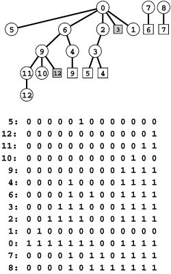
This sequence of row vectors is the transitive closure of the DAG in Figure 19.21, with rows created in reverse topological order, computed as the last action in a recursive DFS function (see Program 19.9). Each row is the logical or of the rows for adjacent vertices, which appear earlier in the list. For example, to compute the row for 0 we take the logical or of the rows for 5, 2, 1, and 6 (and put a 1 corresponding to 0 itself) because the edges 0-5, 0-2, 0-1, and 0-6 take us from 0 to any vertex that is reachable from any of those vertices. We can ignore down edges because they add no new information. For example, we ignore the edge from 0 to 3 because the vertices reachable from 3 are already accounted for in the row corresponding to 2.
Program 19.9 Transitive closure of a DAG
The constructor in this class computes the transitive closure of a DAG with a single DFS. It recursively computes the reachable vertices from each vertex from the reachable vertices of its children in the DFS tree.
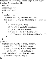
Proof: The proof is immediate by induction from the recursive function in Program 19.9. We visit the vertices in reverse topological order. Every edge points to a vertex for which we have already computed all reachable vertices, and we can therefore compute the set of reachable vertices of any vertex by merging together the sets of reachable vertices associated with the destination vertex of each edge. Taking the logical or of the specified rows in the adjacency matrix accomplishes this merge. We access a row of size V for each tree edge and each cross edge. There are no back edges, and we can ignore down edges because we accounted for any vertices they reach when we processed any ancestors of both nodes earlier in the search.
If our DAG has no down edges (see Exercise 19.42), the running time of Program 19.9 is proportional to V E and represents no improvement over the transitive-closure algorithms that we examined for general digraphs in Section 19.3 (such as, for example, Program 19.4) or the approach based on topological sorting that is described at the beginning of this section. On the other hand, if the number of down edges is large (or, equivalently, the number of cross edges is small), Program 19.9 will be significantly faster than these methods.
The problem of finding an optimal algorithm (one that is guaranteed to finish in time proportional to V2) for computing the transitive closure of dense DAGs is still unsolved. The best known worst-case performance bound is V E. However, we are certainly better off using an algorithm that runs faster for a large class of DAGs, such as Program 19.9, than we are using one that always runs in time proportional to V E, such as Program 19.4. As we see in Section 19.9, this performance improvement for DAGs has direct implications for our ability to compute the transitive closure of general digraphs as well.
Exercises
• 19.115 Show, in the style of Figure 19.27, the reachability vectors that result when we use Program 19.9 to compute the transitive closure of the DAG
3-7 1-4 7-8 0-5 5-2 3-8 2-9 0-6 4-9 2-6 6-4 4-3 2-3.
• 19.116 Develop a version of Program 19.9 that uses a representation of the transitive closure that does not support edge testing and that runs in time proportional to V2 + Σev (e), where the sum is over all edges in the DAG and v (e) is the number of vertices reachable from the destination vertex of edge e. This cost will be significantly less than V E for some sparse DAGs (see Exercise 19.65).
• 19.117 Implement an abstract–transitive-closure class for DAGs that uses extra space at most proportional to V (and is suitable for huge DAGs). Use topological sorting to provide quick response when the vertices are not connected, and use a source-queue implementation to return the length of the path when they are connected.
• 19.118 Develop a transitive-closure implementation based on a sink-queue– based reverse topological sort (see Exercise 19.105).
• 19.119 Does your solution to Exercise 19.118 require that you examine all edges in the DAG, or are there edges that can be ignored, such as the down edges in DFS? Give an example that requires examination of all edges, or characterize the edges that can be skipped.
19.8 Strong Components in Digraphs
Undirected graphs and DAGs are both simpler structures than general digraphs because of the structural symmetry that characterizes the reachability relationships among the vertices: In an undirected graph, if there is a path from s to t, then we know that there is also a path from t to s; in a DAG, if there is a directed path from s to t, then we know that there is no directed path from t to s. For general digraphs, knowing that t is reachable from s gives no information about whether s is reachable from t.
To understand the structure of digraphs, we consider strong connectivity, which has the symmetry that we seek. If s and t are strongly connected (each reachable from the other), then, by definition, so are t and s. As discussed in Section 19.1, this symmetry implies that the vertices of the digraph divide into strong components, which consist of mutually reachable vertices. In this section, we discuss three algorithms for finding the strong components in a digraph.
We use the same interface as for connectivity in our general graph-searching algorithms for undirected graphs (see Program 18.4). The goal of our algorithms is to assign component numbers to each vertex in a vertex-indexed vector, using the labels 0, 1, [triangleright][triangleright][triangleright], for the strong components. The highest number assigned is one less than the number of strong components, and we can use the component numbers to provide a constant-time test of whether two vertices are in the same strong component.
A brute-force algorithm to solve the problem is simple to develop. Using an abstract–transitive-closure ADT, check every pair of vertices s and t to see whether t is reachable from s and s is reachable from t. Define an undirected graph with an edge for each such pair: The connected components of that graph are the strong components of the digraph. This algorithm is simple to describe and to implement, and its running time is dominated by the costs of the abstract–transitive-closure implementation, as described by, say, Property 19.10.
The algorithms that we consider in this section are triumphs of modern algorithm design that can find the strong components of any graph in linear time, a factor of V faster than the brute-force algorithm. For 100 vertices, these algorithms will be 100 times faster than the brute-force algorithm; for 1000 vertices, they will be 1000 times faster; and we can contemplate addressing problems involving billions of vertices. This problem is a prime example of the power of good algorithm design, one which has motivated many people to study graph algorithms closely. Where else might we contemplate reducing resource usage by a factor of 1 billion or more with an elegant solution to an important practical problem?
The history of this problem is instructive ( see reference section ). In the 1950s and 1960s, mathematicians and computer scientists began to study graph algorithms in earnest in a context where the analysis of algorithms itself was under development as a field of study. The broad variety of graph algorithms to be considered—coupled with ongoing developments in computer systems, languages, and our understanding of performing computations efficiently—left many difficult problems unsolved. As computer scientists began to understand many of the basic principles of the analysis of algorithms, they began to understand which graph problems could be solved efficiently and which could not and then to develop increasingly efficient algorithms for the former set of problems. Indeed, R. Tarjan introduced linear-time algorithms for strong connectivity and other graph problems in 1972, the same year that R. Karp documented the intractability of the traveling-salesperson problem and many other graph problems. Tarjan’s algorithm has been a staple of advanced courses in the analysis of algorithms for many years because it solves an important practical problem using simple data structures. In the 1980s, R. Kosaraju took a fresh look at the problem and developed a new solution; people later realized that a paper that describes essentially the same method appeared in the Russian scientific literature in 1972. Then, in 1999, H. Gabow found a simple implementation of one of the first approaches tried in the 1960s, giving a third linear-time algorithm for this problem.
The point of this story is not just that difficult graph-processing problems can have simple solutions, but also that the abstractions that we are using (DFS and adjacency lists) are more powerful than we might realize. As we become more accustomed to using these and similar tools, we should not be surprised to discover simple solutions to other important graph problems as well. Researchers still seek concise implementations like these for numerous other important graph algorithms; many such algorithms remain to be discovered.
Figure 19.28 Computing strong components (Kosaraju’s algorithm)
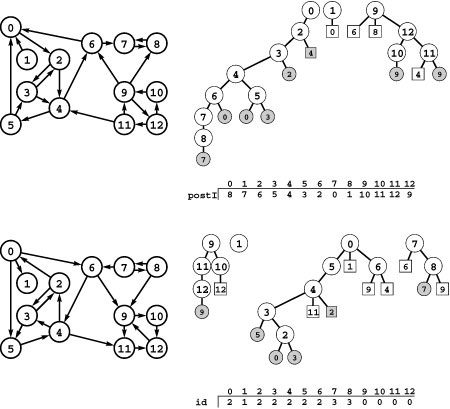
To compute the strong components of the digraph at the lower left, we first do a DFS of its reverse (top left), computing a postorder vector that gives the vertex indices in the order in which the recursive DFS completed (top). This order is equivalent to a postorder walk of the DFS forest (top right). Then we use the reverse of that order to do a DFS of the original digraph (bottom). First we check all nodes reachable from 9, then we scan from right to left through the vector to find that 1 is the rightmost unvisited vertex, so we do the recursive call for 1, and so forth. The trees in the DFS forest that results from this process define the strong components: All vertices in each tree have the same value in the vertex-indexed id vector (bottom).
Kosaraju’s method is simple to explain and implement. To find the strong components of a graph, first run DFS on its reverse, computing the permutation of vertices defined by the postorder numbering. (This process constitutes a topological sort if the digraph is a DAG.) Then, run DFS again on the graph, but to find the next vertex to search (when calling the recursive search function, both at the outset and each time that the recursive search function returns to the top-level search function), use the unvisited vertex with the highest postorder number.
The magic of the algorithm is that, when the unvisited vertices are checked according to the topological sort in this way, the trees in the DFS forest define the strong components just as trees in a DFS forest define the connected components in undirected graphs—two vertices are in the same strong component if and only if they belong
Program 19.10 Strong components (Kosaraju’s algorithm)
Clients can use objects of this class to find the number of strong components of a digraph (count) and to do strong-connectivity tests (stronglyconnected). The SC constructor first builds the reverse di-graph and does a DFS to compute a postorder numbering. Next, it does a DFS of the original digraph, using the reverse of the postorder from the first DFS in the search loop that calls the recursive function. Each recursive call in the second DFS visits all the vertices in a strong component.
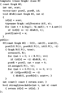
to the same tree in this forest. Figure 19.28 illustrates this fact for our example, and we will prove it in a moment. Therefore, we can assign component numbers as we did for undirected graphs, incrementing the component number each time that the recursive function returns to the top-level search function. Program 19.10 is a full implementation of the method.
Property 19.14 Kosaraju’s method finds the strong components of a graph in linear time and space.
Proof: The method consists of minor modifications to two DFS procedures, so the running time is certainly proportional to V2 for dense graphs and V + E for sparse graphs (using an adjacency-lists representation), as usual. To prove that it computes the strong components properly, we have to prove that two vertices s and t are in the same tree in the DFS forest for the second search if and only if they are mutually reachable.
If s and t are mutually reachable, they certainly will be in the same DFS tree because when the first of the two is visited, the second is unvisited and is reachable from the first and so will be visited before the recursive call for the root terminates.
To prove the converse, we assume that s and t are in the same tree, and let r be the root of the tree. The fact that s is reachable from r (through a directed path of tree edges) implies that there is a directed path from s to r in the reverse digraph. Now, the key to the proof is that there must also be a path from r to s in the reverse digraph because r has a higher postorder number than s (since r was chosen first in the second DFS at a time when both were unvisited) and there is a path from s to r: If there were no path from r to s, then the path from s to r in the reverse would leave s with a higher postorder number. Therefore, there are directed paths from s to r and from r to s in the digraph and its reverse: s and r are strongly connected. The same argument proves that t and r are strongly connected, and therefore s and t are strongly connected.
The implementation for Kosaraju’s algorithm for the adjacency-matrix digraph representation is even simpler than Program 19.10 because we do not need to compute the reverse explicitly; that problem is left as an exercise (see Exercise 19.125).
Program 19.11 Strong components (Tarjan’s algorithm)
This DFS class is another implementation of the same interface as Program 19.10. It uses a stack S to hold each vertex until determining that all the vertices down to a certain point at the top of the stack belong to the same strong component. The vertex-indexed vector low keeps track of the lowest preorder number reachable via a series of down links followed by one up link from each node ( see text ).
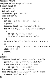
Program 19.10 represents an optimal solution to the strong-connectivity problem that is analogous to our solutions for connectivity in Chapter 18. In Section 19.9, we examine the task of extending this solution to compute the transitive closure and to solve the reachability (abstract–transitive-closure) problem for digraphs.
First, however, we consider Tarjan’s algorithm and Gabow’s algorithm—ingenious methods that require only a few simple modifications to our basic DFS procedure. They are preferable to Kosaraju’s algorithm because they use only one pass through the graph and because they do not require computation of the reverse for sparse graphs.
Tarjan’s algorithm is similar to the program that we studied in Chapter 17 for finding bridges in undirected graphs (see Program 18.7). The method is based on two observations that we have already made in other contexts. First, we consider the vertices in reverse topological order so that when we reach the end of the recursive function for a vertex we know we will not encounter any more vertices in the same strong component (because all the vertices that can be reached from that vertex have been processed). Second, the back links in the tree provide a second path from one vertex to another and bind together the strong components.
The recursive DFS function uses the same computation as Program 18.7 to find the highest vertex reachable (via a back edge) from any descendant of each vertex. It also uses a vertex-indexed vector to keep track of the strong components and a stack to keep track of the current search path. It pushes the vertex names onto a stack on entry to the recursive function, then pops them and assigns component numbers after visiting the final member of each strong component. The algorithm is based on our ability to identify this moment with a simple test (based on keeping track of the highest ancestor reachable via one up link from all descendants of each node) at the end of the recursive procedure that tells us that all vertices encountered since entry (except those already assigned to a component) belong to the same strong component.
The implementation in Program 19.11 is a succinct and complete description of the algorithm that fills in the details missing from the brief sketch just given. Figure 19.29 illustrates the operation of the algorithm for our sample digraph from Figure 19.1.
Figure 19.29 Computing strong components (Tarjan and Gabow algorithms)
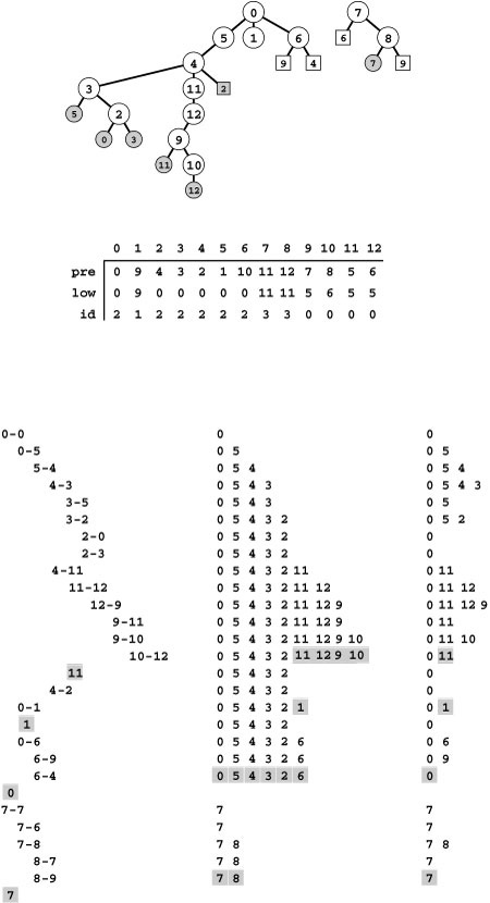
Tarjan’s algorithm is based on a recursive DFS, augmented to push vertices on a stack. It computes a component index for each vertex in a vertex-indexed vector id, using auxiliary vectors pre and low (center). The DFS tree for our sample graph is shown at the top and an edge trace at the bottom left. In the center at the bottom is the main stack: We push vertices reached by tree edges. Using a DFS to consider the vertices in reverse topological order, we compute, for each v, the highest point reachable via a back link from an ancestor (low[v]). When a vertex v has pre[v] = low[v] (vertices 11, 1, 0, and 7 here) we pop it and all the vertices above it (shaded) and assign them all the next component number.
In Gabow’s algorithm, we push vertices on the main stack, just as in Tarjan’s algorithm, but we also keep a second stack (bottom right) with vertices on the search path that are known to be in different strong components, by popping all vertices after the destination of each back edge. When we complete a vertex v with v at the top of this second stack (shaded), we know that all vertices above v on the main stack are in the same strong component.
Property 19.15 Tarjan’s algorithm finds the strong components of a digraph in linear time.
Proof sketch: If a vertex s has no descendants or up links in the DFS tree, or if it has a descendant in the DFS tree with an up link that points to s and no descendants with up links that point higher up in the tree, then it and all its descendants (except those vertices that satisfy the same property and their descendants) constitute a strong component. To establish this fact, we note that every descendant t of s that does not satisfy the stated property has some descendant that has an up link pointing higher than t in the tree. There is a path from s to t down through the tree and we can find a path from t to s as follows: Go down from t to the vertex with the up link that reaches past t, then continue the same process from that vertex until reaching s.
As usual, the method is linear time because it consists of adding a few constant-time operations to a standard DFS.
In 1999 Gabow discovered the version of Tarjan’s algorithm in Program 19.12. The algorithm maintains the same stack of vertices in the same way as does Tarjan’s algorithm, but it uses a second stack (instead of a vertex-indexed vector of preorder numbers) to decide when to pop all the vertices in each strong component from the main stack. The second stack contains vertices on the search path. When a back edge shows that a sequence of such vertices all belong to the same strong component, we pop that stack to leave only the destination vertex of the back edge, which is nearer the root of the tree than are any of the other vertices. After processing all the edges for each vertex (making recursive calls for the tree edges, popping the path stack for the back edges, and ignoring the down edges), we check to see whether the current vertex is at the top of the path stack. If it is, it and all the vertices above it on the main stack make a strong component, and we pop them and assign the next strong component number to them, as we did in Tarjan’s algorithm.
The example in Figure 19.29 also shows the contents of this second stack. Thus, this figure also illustrates the operation of Gabow’s algorithm.
Property 19.16 Gabow’s algorithm finds the strong components of a digraph in linear time.
Program 19.12 Strong components (Gabow’s algorithm)
This alternate implementation of the recursive member function in Program 19.11 uses a second stack path instead of the vertex-indexed vector low to decide when to pop the vertices in each strong component from the main stack ( see text ).
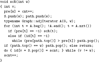
Formalizing the argument just outlined and proving the relationship between the stack contents that it depends upon is an instructive exercise for mathematically inclined readers (see Exercise 19.132). As usual, the method is linear time because it consists of adding a few constant-time operations to a standard DFS.
The strong-components algorithms that we have considered in this section are all ingenious and are deceptively simple. We have considered all three because they are testimony to the power of fundamental data structures and carefully crafted recursive programs. From a practical standpoint, the running time of all the algorithms is proportional to the number of edges in the digraph, and performance differences are likely to be dependent upon implementation details. For example, pushdown-stack ADT operations constitute the inner loop of Tarjan’s and Gabow’s algorithm. Our implementations use the bare-bones stack class implementations of Chapter 4; implementations that use STL stacks, which do error-checking and carry other overhead, may be slower. The implementation of Kosaraju’s algorithm is perhaps the simplest of the three, but it suffers the slight disadvantage (for sparse digraphs) of requiring three passes through the edges (one to make the reverse and two DFS passes).
Next, we consider a key application of computing strong components: building an efficient reachability (abstract–transitive-closure) ADT for digraphs.
Exercises
• 19.120 Describe what happens when you use Kosaraju’s algorithm to find the strong components of a DAG.
• 19.121 Describe what happens when you use Kosaraju’s algorithm to find the strong components of a digraph that consists of a single cycle.
•• 19.122 Can we avoid computing the reverse of the digraph in the adjacency-lists version of Kosaraju’s method (Program 19.10) by using one of the three techniques mentioned in Section 19.4 for avoiding the reverse computation when doing a topological sort? For each technique, give either a proof that it works or a counterexample that shows that it does not work.
• 19.123 Show, in the style of Figure 19.28, the DFS forests and the contents of the auxiliary vertex-indexed vectors that result when you use Kosaraju’s algorithm to compute the strong components of the reverse of the digraph in Figure 19.5. (You should have the same strong components.)
19.124 Show, in the style of Figure 19.28, the DFS forests and the contents of the auxiliary vertex-indexed vectors that result when you use Kosaraju’s algorithm to compute the strong components of the digraph
3-7 1-4 7-8 0-5 5-2 3-8 2-9 0-6 4-9 2-6 6-4.
• 19.125 Implement Kosaraju’s algorithm for finding the strong components of a digraph for a digraph representation that suports edge existence testing. Do not explicitly compute the reverse. Hint: Consider using two different recursive DFS functions.
• 19.126 Describe what happens when you use Tarjan’s algorithm to find the strong components of a DAG.
• 19.127 Describe what happens when you use Tarjan’s algorithm to find the strong components of a digraph that consists of a single cycle.
• 19.128 Show, in the style of Figure 19.29, the DFS forest, stack contents during the execution of the algorithm, and the final contents of the auxiliary vertex-indexed vectors that result when you use Tarjan’s algorithm to compute the strong components of the reverse of the digraph in Figure 19.5. (You should have the same strong components.)
19.129 Show, in the style of Figure 19.29, the DFS forest, stack contents during the execution of the algorithm, and the final contents of the auxiliary vertex-indexed vectors that result when you use Tarjan’s algorithm to compute the strong components of the digraph
3-7 1-4 7-8 0-5 5-2 3-8 2-9 0-6 4-9 2-6 6-4.
• 19.130 Modify the implementations of Tarjan’s algorithm in Program 19.11 and of Gabow’s algorithm in Program 19.12 such that they use sentinel values to avoid the need to check explicitly for cross links.
19.131 Show, in the style of Figure 19.29, the DFS forest, contents of both stacks during the execution of the algorithm, and the final contents of the auxiliary vertex-indexed vectors that result when you use Gabow’s algorithm to compute the strong components of the digraph
3-7 1-4 7-8 0-5 5-2 3-8 2-9 0-6 4-9 2-6 6-4.
• 19.132 Give a full proof of Property 19.16.
• 19.133 Develop a version of Gabow’s algorithm that finds bridges and edge-connected components in undirected graphs.
• 19.134 Develop a version of Gabow’s algorithm that finds articulation points and biconnected components in undirected graphs.
19.135 Develop a table in the spirit of Table 18.1 to study strong connectivity in random digraphs (see Table 19.2). Let S be the set of vertices in the largest strong component. Keep track of the size of S and study the percentages of edges in the following four classes: those connecting two vertices in S, those pointing out of S, those pointing in to S, those connecting two vertices not in S.
19.136 Run empirical tests to compare the brute-force method for computing strong components described at the beginning of this section, Kosaraju’s algorithm, Tarjan’s algorithm, and Gabow’s algorithm, for various types of digraphs (see Exercises 19.11–18).
••• 19.137 Develop a linear-time algorithm for strong 2-connectivity: Determine whether a strongly connected digraph has the property that it remains strongly connected after removing any vertex (and all its incident edges).
19.9 Transitive Closure Revisited
By putting together the results of the previous two sections, we can develop an algorithm to solve the abstract–transitive-closure problem for digraphs that—although it offers no improvement over a DFS-based solution in the worst case—will provide an optimal solution in many situations.
The algorithm is based on preprocessing the digraph to build the latter’s kernel DAG (see Property 19.2). The algorithm is efficient if the kernel DAG is small relative to the size of the original digraph. If the digraph is a DAG (and therefore is identical to its kernel DAG) or if it has just a few small cycles, we will not see any significant cost savings; however, if the digraph has large cycles or large strong components (and therefore a small kernel DAG), we can develop optimal or near-optimal algorithms. For clarity, we assume the kernel DAG to be sufficiently small that we can afford an adjacency-matrix representation, although the basic idea is still effective for larger kernel DAGs.
To implement the abstract transitive closure, we preprocess the digraph as follows:
• Find its strong components
• Build its kernel DAG
• Compute the transitive closure of the kernel DAG
We can use Kosaraju’s, Tarjan’s, or Gabow’s algorithm to find the strong components; a single pass through the edges to build the kernel DAG (as described in the next paragraph); and DFS (Program 19.9) to compute its transitive closure. After this preprocessing, we can immediately access the information necessary to determine reachability.
Once we have a vertex-indexed vector with the strong components of a digraph, building an adjacency-matrix representation of its kernel DAG is a simple matter. The vertices of the DAG are the component numbers in the digraph. For each edge s-t in the original digraph, we simply set D->adj[sc[s]][sc[t]] to 1. We would have to cope with duplicate edges in the kernel DAG if we were using an adjacency-lists representation—in an adjacency matrix, duplicate edges simply correspond to setting to 1 a matrix entry that has already been set to 1. This small point is significant because the number of duplicate edges is potentially huge (relative to the size of the kernel DAG) in this application.
Property 19.17 Given two vertices s and t in a digraph D, let sc ( s ) and sc ( t ) , respectively, be their corresponding vertices in D’s kernel DAG K. Then, t is reachable from s in D if and only if sc ( t ) is reachable from sc ( s ) in K.
This simple fact follows from the definitions. In particular, this property assumes the convention that a vertex is reachable from itself (all vertices have self-loops). If the vertices are in the same strong component ( sc ( s ) = sc ( t )), then they are mutually reachable.
Program 19.13 Strong-component–based transitive closure
This class implements the (abstract) transitive closure interface for di-graphs by computing the strong components (using, say Program 19.11), kernel DAG, and the transitive closure of the kernel DAG (using Program 19.9). It assumes that class SC has a public member function ID that returns the strong component index (from the id array) for any given vertex. These numbers are the vertex indices in the kernel DAG. A vertex t is reachable from a vertex s in the digraph if and only if ID(t) is reachable from ID(s) in the kernel DAG.
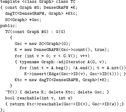
We determine whether a given vertex t is reachable from a given vertex s inthesamewayaswebuiltthekernelDAG:Weusethevertex-indexed vector computed by the strong-components algorithm to get the component numbers sc ( s ) and sc ( t ) (in constant time), which we interpret as abstract vertex indices for the kernel DAG. Using them as vertex indices for the transitive closure of the kernel DAG tells us the result.
Program 19.13 is an implementation of the abstract–transitive-closure ADT that embodies these ideas. We use an abstract –transitive-closure interface for the kernel DAG as well. The running time of this implementation depends not just on the number of vertices and edges in the digraph but also on properties of its kernel DAG. For purposes of analysis, we suppose that we use an adjacency-matrix representation for the kernel DAG because we expect the kernel DAG to be small, if not also dense.
Property 19.18 We can support constant query time for the abstract transitive closure of a digraph with space proportional to V + V2 and time proportional to E + V2 + vx for preprocessing (computing the transitive closure), where v is the number of vertices in the kernel DAG and x is the number of cross edges in its DFS forest.
Proof: Immediate from Property 19.13.
If the digraph is a DAG, then the strong-components computation provides no new information, and this algorithm is the same as Program 19.9; in general digraphs that have cycles, however, this algorithm is likely to be significantly faster than Warshall’s algorithm or the DFS-based solution. For example, Property 19.18 immediately implies the following result.
Property 19.19 We can support constant query time for the abstract transitive closure of any digraph whose kernel DAG has less than ![]() vertices with space proportional to V and time proportional to E + V for preprocessing.
vertices with space proportional to V and time proportional to E + V for preprocessing.
Proof:Take v < ![]() in Property 19.18 and note that x < v2.
in Property 19.18 and note that x < v2.
We might consider other variations on these bounds. For example, if we are willing to use space proportional to E, we can achieve the same time bounds when the kernel DAG has up to ![]() vertices. Moreover, these time bounds are conservative because they assume that the kernel DAG is dense with cross edges—and certainly it need not be so.
vertices. Moreover, these time bounds are conservative because they assume that the kernel DAG is dense with cross edges—and certainly it need not be so.
The primary limiting factor in the applicability of this method is the size of the kernel DAG. The more similar our digraph is to a DAG (the larger its kernel DAG), the more difficulty we face in computing its transitive closure. Note that (of course) we still have not violated the lower bound implicit in Property 19.9, since the algorithm runs in time proportional to V3 for dense DAGs; we have, however, significantly broadened the class of graphs for which we can avoid this worst-case performance. Indeed, constructing a random-digraph model that produces digraphs for which the algorithm is slow is a challenge (see Exercise 19.142).
Table 19.2 Properties of random digraphs
This table shows the numbers of edges and vertices in the kernel DAGs for random digraphs generated from two different models (the directed versions of the models in Table 18.1). In both cases, the kernel DAG becomes small (and is sparse) as the density increases.
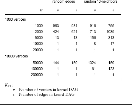
Table 19.2 displays the results of an empirical study; it shows that random digraphs have small kernel DAGs even for moderate densities and even in models with severe restrictions on edge placement. Although there can be no guarantees in the worst case, we can expect to see huge digraphs with small kernel DAGs in practice. When we do have such a digraph, we can provide an efficient implementation of the abstract–transitive-closure ADT.
Exercises
• 19.138 Develop a version of the implementation of the abstract transitive closure for digraphs based on using a sparse-graph representation of the kernel DAG. Your challenge is to eliminate duplicates on the list without using an excessive amount of time or space (see Exercise 19.65).
• 19.139 Show the kernel DAG computed by Program 19.13 and its transitive closure for the digraph
3-7 1-4 7-8 0-5 5-2 3-8 2-9 0-6 4-9 2-6 6-4.
• 19.140 Convert the strong-component–based abstract–transitive-closure implementation (Program 19.13) into an efficient program that computes the adjacency matrix of the transitive closure for a digraph represented with an adjacency matrix, using Gabow’s algorithm to compute the strong components and the improved Warshall’s algorithm to compute the transitive closure of the DAG.
19.141 Do empirical studies to estimate the expected size of the kernel DAG for various types of digraphs (see Exercises 19.11–18).
•• 19.142 Develop a random-digraph model that generates digraphs that have large kernel DAGs. Your generator must generate edges one at a time, but it must not make use of any structural properties of the resulting graph.
19.143 Develop an implementation of the abstract transitive closure in a digraph by finding the strong components and building the kernel DAG, then answering reachability queries in the affirmative if the two vertices are in the same strong component, and doing a DFS in the DAG to determine reachability otherwise.
19.10 Perspective
In this chapter, we have considered algorithms for solving the topological-sorting, transitive-closure, and shortest-paths problems for digraphs and for DAGs, including fundamental algorithms for finding cycles and strong components in digraphs. These algorithms have numerous important applications in their own right and also serve as the basis for the more difficult problems involving weighted graphs that we consider in the next two chapters. Worst-case running times of these algorithms are summarized in Table 19.3.
In particular, a common theme through the chapter has been the solution of the abstract–transitive-closure problem, where we wish
Table 19.3 Worst-case cost of digraph-processing operations
This table summarizes the cost (worst-case running time) of algorithms for various digraph-processing problems considered in this chapter, for random graphs and graphs where edges randomly connect each vertex to one of 10 specified neighbors. All costs assume use of the adjacency-list representation; for the adjacency-matrix representation the E entries become V2 entries, so, for example, the cost of computing all shortest paths is V3. The linear-time algorithms are optimal, so the costs will reliably predict the running time on any input; the others may be overly conservative estimates of cost, so the running time may be lower for certain types of graphs. Performance characteristics of the fastest algorithms for computing the transitive closure of a digraph depend on the digraph’s structure, particularly the size of its kernel DAG.
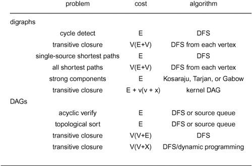
to support an ADT that can determine quickly, after preprocessing, whether there is a directed path from one given vertex to another. Despite a lower bound that implies that our worst-case preprocessing costs are significantly higher than V2, the method discussed in Section 19.7 melds the basic methods from throughout the chapter into a simple solution that provides optimal performance for many types of digraphs—the significant exception being dense DAGs. The lower bound suggests that better guaranteed performance on all graphs will be difficult to achieve, but we can use these methods to get good performance on practical graphs.
The goal of developing an algorithm with performance characteristics similar to the union-find algorithms of Chapter 1 for dense di-graphs remains elusive. Ideally, we would like to define an ADT where we can add directed edges or test whether one vertex is reachable from another and to develop an implementation where we can support all the operations in constant time (see Exercises 19.153 through 19.155). As discussed in Chapter 1, we can come close to that goal for undirected graphs, but comparable solutions for digraphs or DAGs are still not known. (Note that removing edges presents a challenge even for undirected graphs.) Not only does this dynamic reachability problem have both fundamental appeal and direct application in practice, but also it plays a critical role in the development of algorithms at a higher level of abstraction. For example, reachability lies at the heart of the problem of implementing the network simplex algorithm for the min-cost flow problem, a problem-solving model of wide applicability that we consider in Chapter 22.
Many other algorithms for processing digraphs and DAGs have important practical applications and have been studied in detail, and many digraph-processing problems still call for the development of efficient algorithms. The following list is representative.
Dominators Given a DAG with all vertices reachable from a single source r, a vertex s dominates a vertex t if every path from r to t contains s. (In particular, each vertex dominates itself.) Every vertex v other than the source has an immediate dominator that dominates v but does not dominate any dominator of v but v and itself. The set of immediate dominators is a tree that spans all vertices reachable from the source. This structure is important in compiler implementations. The dominator tree can be computed in linear time with a DFS-based approach that uses several ancillary data structures, although a slightly slower version is typically used in practice.
Transitive reduction Given a digraph, find a digraph that has the same transitive closure and the smallest number of edges among all such digraphs. This problem is tractable (see Exercise 19.150); but if we restrict it to insist that the result be a subgraph of the original graph, it is NP-hard.
Directed Euler path Given a digraph, is there a directed path connecting two given vertices that uses each edge in the digraph exactly once? This problem is easy by essentially the same arguments as for the corresponding problem for undirected graphs, which we considered in Section 17.7 (see Exercise 17.92).
Directed mail carrier Given a digraph, find a directed tour with a minimal number of edges that uses every edge in the graph at least once (but is allowed to use edges multiple times). As we shall see in Section 22.7, this problem reduces to the mincost-flow problem and is therefore tractable.
Directed Hamilton path Find the longest simple directed path in a digraph. This problem is NP-hard, but it is easy if the digraph is a DAG (see Exercise 19.114).
Uniconnected subgraph A digraph is said to be uniconnected if there is at most one directed path between any pair of vertices. Given a digraph and an integer k, determine whether there is a uniconnected subgraph with at least k edges. This problem is known to be NP-hard for general k.
Feedback vertex set Decide whether a given digraph has a subset of at most k vertices that contains at least one vertex from every directed cycle in G. This problem is known to be NP-hard.
Even cycle Decide whether a given digraph has a cycle of even length. As mentioned in Section 17.8, this problem, while not intractable, is so difficult to solve that no one has yet devised an algorithm that is useful in practice.
Just as for undirected graphs, myriad digraph-processing problems have been studied, and knowing whether a problem is easy or intractable is often a challenge (see Section 17.8). As indicated throughout this chapter, some of the facts that we have discovered about digraphs are expressions of more general mathematical phenomena, and many of our algorithms have applicability at levels of abstraction different from that at which we have been working. On the one hand, the concept of intractability tells us that we might encounter fundamental roadblocks in our quest for efficient algorithms that can guarantee efficient solutions to some problems. On the other hand, the classic algorithms described in this chapter are of fundamental importance and have broad applicability, as they provide efficient solutions to problems that arise frequently in practice and would otherwise be difficult to solve.
Exercises
19.144 Adapt Programs 17.18 and 17.19 to implement an ADT function for printing an Euler path in a digraph, if one exists. Explain the purpose of any additions or changes that you need to make in the code.
• 19.145 Draw the dominator tree of the digraph
3-7 1-4 7-8 0-5 5-2 3-0 2-9 0-6 4-9 2-6
6-4 1-5 8-2 9-0 8-3 4-5 2-3 1-6 3-5 7-6.
•• 19.146 Write class that uses DFS to create a parent-link representation of the dominator tree of a given digraph ( see reference section ).
• 19.147 Find a transitive reduction of the digraph
3-7 1-4 7-8 0-5 5-2 3-0 2-9 0-6 4-9 2-6
6-4 1-5 8-2 9-0 8-3 4-5 2-3 1-6 3-5 7-6.
• 19.148 Find a subgraph of the digraph
3-7 1-4 7-8 0-5 5-2 3-0 2-9 0-6 4-9 2-6
6-4 1-5 8-2 9-0 8-3 4-5 2-3 1-6 3-5 7-6
that has the same transitive closure and the smallest number of edges among all such subgraphs.
• 19.149 Prove that every DAG has a unique transitive reduction, and give an efficient ADT function implementation for computing the transitive reduction of a DAG.
• 19.150 Write an efficient ADT function for digraphs that computes a transitive reduction.
19.151 Give an algorithm that determines whether or not a given digraph is uniconnected. Your algorithm should have a worst-case running time proportional to V E.
19.152 Find the largest uniconnected subgraph in the digraph
3-7 1-4 7-8 0-5 5-2 3-0 2-9 0-6 4-9 2-6
6-4 1-5 8-2 9-0 8-3 4-5 2-3 1-6 3-5 7-6.
• 19.153 Develop a digraph class implemention that supports inserting an edge, removing an edge, and testing whether two vertices are in the same strong component, such that construction, edge insertion, and edge removal all take linear time and strong-connectivity queries take constant time, in the worst case.
• 19.154 Solve Exercise 19.153, in such a way that edge insertion, edge removal, and strong-connectivity queries all take time proportional to log V in the worst case.
••• 19.155 Solve Exercise 19.153, in such a way that edge insertion, edge removal, and strong-connectivity queries all take near-constant time (as they do for the union-find algorithms for connectivity in undirected graphs).