CHAPTER TWENTY-ONE
Shortest Paths

EVERY PATH IN a weighted digraph has an associated path weight, the value of which is the sum of the weights of that path’s edges. This essential measure allows us to formulate such problems as “find the lowest-weight path between two given vertices.” These shortest-paths problems are the topic of this chapter. Not only are shortest-paths problems intuitive for many direct applications, but they also take us into a powerful and general realm where we seek efficient algorithms to solve general problems that can encompass a broad variety of specific applications.

Several of the algorithms that we consider in this chapter relate directly to various algorithms that we examined in Chapters 17 through 20. Our basic graph-search paradigm applies immediately, and several of the specific mechanisms that we used in Chapters 17 and 19 to address connectivity in graphs and digraphs provide the basis for us to solve shortest-paths problems.

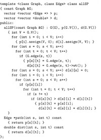
For economy, we refer to weighted digraphs as networks. Figure 21.1 shows a sample network, with standard representations. We have already developed an ADT interface with adjacency-matrix and adjacency-lists class implementations for networks in Section 20.1—we just pass true as a second argument when we call the constructor so that the class keeps one representation of each edge, precisely as we did when deriving digraph representations in Chapter 19 from the undirected graph representations in Chapter 17 (see Programs 20.1 through 20.4).

As discussed at length in Chapter 20, we use pointers to abstract edges for weighted digraphs to broaden the applicability of our implementations. This approach has certain implications that are different

Figure 21.1 Sample network and representations

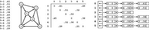
This network (weighted digraph) is shown in four representations: list of edges, drawing, adjacency matrix, and adjacency lists (left to right). As we did for MST algorithms, we show the weights in matrix entries and in list nodes, but use edge pointers in our programs. While we often use edge weights that are proportional to their lengths in the drawing (as we did for MST algorithms), we do not insist on this rule because most shortest-paths algorithms handle arbitrary nonnegative weights (negative weights do present special challenges). The adjacency matrix is not symmetric, and the adjacency lists contain one node for each edge (as in unweighted digraphs). Nonexistent edges are represented by null pointers in the matrix (blank in the figure) and are not present at all in the lists. Self-loops of length 0 are present because they simplify our implementations of shortest-paths algorithms. They are omitted from the list of edges at left for economy and to indicate the typical scenario where we add them by convention when we create an adjacency-matrix or adjacency-lists representation.

for digraphs than the ones that we considered for undirected graphs in Section 20.1 and are worth noting. First, since there is only one representation of each edge, we do not need to use the from function in the edge class (see Program 20.1) when using an iterator: In a digraph, e->from(v) is true for every edge pointer e feturn by an iterator for v. Second, as we saw in Chapter 19, it is often useful when processing a digraph to be able to work with its reverse graph, but we need a different approach than that taken by Program 19.1, because that implementation creates edges to create the reverse, and we assume that a graph ADT whose clients provide pointers to edges should not create edges on its own (see Exercise 21.3).

In applications or systems for which we need all types of graphs, it is a textbook exercise in software engineering to define a network ADT from which ADTs for the unweighted undirected graphs of Chapters 17 and 18, the unweighted digraphs of Chapter 19, or the weighted undirected graphs of Chapter 20 can be derived (see Exercise 21.10).

When we work with networks, it is generally convenient to keep self-loops in all the representations. This convention allows algorithms the flexibility to use a sentinel maximum-value weight to indicate that a vertex cannot be reached from itself. In our examples, we use self-loops of weight 0, although positive-weight self-loops certainly make sense in many applications. Many applications also call for parallel edges, perhaps with differing weights. As we mentioned in Section 20.1, various options for ignoring or combining such edges are appropriate in various different applications. In this chapter, for simplicity, none of our examples use parallel edges, and we do not allow parallel edges in the adjacency-matrix representation; we also do not check for parallel edges or remove them in adjacency lists.

All the connectivity properties of digraphs that we considered in Chapter 19 are relevant in networks. In that chapter, we wished to

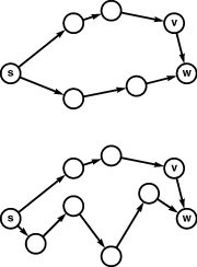
Figure 21.2 Shortest-path trees

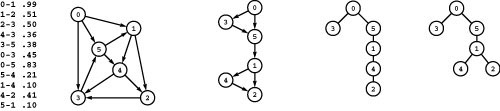
A shortest-path tree (SPT) defines shortest paths from the root to other vertices (see Definition 21.2). In general, different paths may have the same length, so there may be multiple SPTs defining the shortest paths from a given vertex. In the example network shown at left, all shortest paths from 0 are subgraphs of the DAG shown to the right of the network. A tree rooted at 0 spans this DAG if and only if it is an SPT for 0. The two trees at right are such trees.

know whether it is possible to get from one vertex to another; in this chapter, we take weights into consideration—we wish to find the best way to get from one vertex to another.

Definition 21.1A shortest path between two vertices s and t in a network is a directed simple path from s to t with the property that no other such path has a lower weight.

This definition is succinct, but its brevity masks points worth examining. First, if t is not reachable from s, there is no path at all, and therefore there is no shortest path. For convenience, the algorithms that we consider often treat this case as equivalent to one in which there exists an infinite-weight path from s to t. Second, as we did for MST algorithms, we use networks where edge weights are proportional to edge lengths in examples, but the definition has no such requirement and our algorithms (other than the one in Section 21.5) do not make this assumption. Indeed, shortest-paths algorithms are at their best when they discover counterintuitive shortcuts, such as a path between two vertices that passes through several other vertices but has total weight smaller than that of a direct edge connecting those vertices. Third, there may be multiple paths of the same weight from one vertex to another; we typically are content to find one of them. Figure 21.2 shows an example with general weights that illustrates these points.

The restriction in the definition to simple paths is unnecessary in networks that contain edges that have nonnegative weight, because any cycle in a path in such a network can be removed to give a path that is no longer (and is shorter unless the cycle comprises zero-weight edges). But when we consider networks with edges that could have negative weight, the need for the restriction to simple paths is readily apparent: Otherwise, the concept of a shortest path is meaningless if there is a cycle in the network that has negative weight. For example, suppose that the edge 3-5 in the network in Figure 21.1 were to have weight -.38, andedge 5-1 were to have weight -.31. Then, the weight of the cycle 1-4-3-5-1 would be .32 + .36 - .38 - .31 = -.01, and we could spin around that cycle to generate arbitrarily short paths. Note carefully that, as is true in this example, it is not necessary for all the edges on a negative-weight cycle to be of negative weight; what counts is the sum of the edge weights. For brevity, we use the term negative cycle to refer to directed cycles whose total weight is negative.

In the definition, suppose that some vertex on a path from s to t is also on a negative cycle. In this case, the existence of a (nonsimple) shortest path from s to t would be a contradiction, because we could use the cycle to construct a path that had a weight lower than any given value. To avoid this contradiction, we restrict to simple paths in the definition so that the concept of a shortest path is well defined in any network. However, we do not consider negative cycles in networks until Section 21.7, because, as we see there, they present a truly fundamental barrier to the solution of shortest-paths problems.

To find shortest paths in a weighted undirected graph, we build a network with the same vertices and with two edges (one in each direction) corresponding to each edge in the graph. There is a one-to-one correspondence between simple paths in the network and simple paths in the graph, and the costs of the paths are the same; so shortest-paths problems are equivalent. Indeed, we build precisely such a network when we build the standard adjacency-lists or adjacency-matrix representation of a weighted undirected graph (see, for example, Figure 20.3). This construction is not helpful if weights can be negative, because it gives negative cycles in the network, and we do not know how to solve shortest-paths problems in networks that have negative cycles (see Section 21.7). Otherwise, the algorithms for networks that we consider in this chapter also work for weighted undirected graphs.

In certain applications, it is convenient to have weights on vertices instead of, or in addition to, weights on edges; and we might also consider more complicated problems where both the number of edges on the path and the overall weight of the path play a role. We can handle such problems by recasting them in terms of edge-weighted networks (see, for example, Exercise 21.4) or by slightly extending the basic algorithms (see, for example, Exercise 21.52).

Figure 21.3 All shortest paths

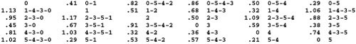
This table gives all the shortest paths in the network of Figure 21.1 and their lengths. This network is strongly connected, so there exist paths connecting each pair of vertices.

The goal of a source-sink shortest-path algorithm is to compute one of the entries in this table; the goal of a single-source shortest-paths algorithm is to compute one of the rows in this table; and the goal of an all-pairs shortest-paths algorithm is to compute the whole table. Generally, we use more compact representations, which contain essentially the same information and allow clients to trace any path in time proportional to its number of edges (see Figure 21.8).

Because the distinction is clear from the context, we do not introduce special terminology to distinguish shortest paths in weighted graphs from shortest paths in graphs that have no weights (where a path’s weight is simply its number of edges—see Section 17.7). The usual nomenclature refers to (edge-weighted) networks, as used in this chapter, since the special cases presented by undirected or unweighted graphs are handled easily by algorithms that process networks.

We are interested in the same basic problems that we defined for undirected and unweighted graphs in Section 18.7. We restate them here, noting that Definition 21.1 implicitly generalizes them to take weights into account in networks.

Source–sink shortest path Given a start vertex s and a finish vertex t, find a shortest path in the graph from s to t. We refer to the start vertex as the source and to the finish vertex as the sink, except in contexts where this usage conflicts with the definition of sources (vertices with no incoming edges) and sinks (vertices with no outgoing edges) in digraphs.

Single-source shortest paths Given a start vertex s, find shortest paths from s to each other vertex in the graph.

All-pairs shortest paths Find shortest paths connecting each pair of vertices in the graph. For brevity, we sometimes use the term all shortest paths to refer to this set of V² paths.

If there are multiple shortest paths connecting any given pair of vertices, we are content to find any one of them. Since paths have varying number of edges, our implementations provide member functions that allow clients to trace paths in time proportional to the paths’ lengths. Any shortest path also implicitly gives us the shortest-path length, but our implementations explicitly provide lengths. In summary, to be precise, when we say “find a shortest path” in the problem statements just given, we mean “compute the shortest-path length and a way to trace a specific path in time proportional to that path’s length.”

Figure 21.3 illustrates shortest paths for the example network in Figure 21.1. In networks with V vertices, we need to specify V paths to solve the single-source problem, and to specify V² paths to solve the all-pairs problem. In our implementations, we use a representation more compact than these lists of paths; we first noted it in Section 18.7, and we consider it in detail in Section 21.1.

In C++ implementations, we build our algorithmic solutions to these problems into ADT implementations that allow us to build efficient client programs that can solve a variety of practical graph-processing problems. For example, as we see in Section 21.3, we implement solutions to the all-pairs shortest-paths classes as constructors within classes that support constant-time shortest-path queries. We also build classes to solve single-source problems so that clients who need to compute shortest paths from a specific vertex (or a small set of them) can avoid the expense of computing shortest paths for other vertices. Careful consideration of such issues and proper use of the algorithms that we examine can mean the difference between an efficient solution to a practical problem and a solution that is so costly that no client could afford to use it.

Shortest-paths problems arise in various guises in numerous applications. Many of the applications appeal immediately to geometric intuition, but many others involve arbitrary cost structures. As we did with minimum spanning trees (MSTs) in Chapter 20, we sometimes take advantage of geometric intuition to help develop an understanding of algorithms that solve the problems but stay cognizant that our algorithms operate properly in more general settings. In Section 21.5, we do consider specialized algorithms for Euclidean networks. More important, in Sections 21.6 and 21.7, we see that the basic algorithms are effective for numerous applications where networks represent an abstract model of the computation.

Road maps Tables that give distances between all pairs of major cities are a prominent feature of many road maps. We presume that the map maker took the trouble to be sure that the distances are the shortest ones, but our assumption is not necessarily always valid (see, for example, Exercise 21.11). Generally, such tables are for undirected graphs that we should treat as networks with edges in both directions corresponding to each road, though we might contemplate handling one-way streets for city maps and some similar applications.

Figure 21.4 Distances and paths

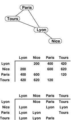
Road maps typically contain distance tables like the one in the center for this tiny subset of French cities connected by highways as shown in the graph at the top. Though rarely found in maps, a table like the one at the bottom would also be useful, as it tells what signs to follow to execute the shortest path. For example, to decide how to get from Paris to Nice, we can check the table, which says to begin by following signs to Lyon.

As we see in Section 21.3, it is not difficult to provide other useful information, such as a table that tells how to execute the shortest paths (see Figure 21.4). In modern applications, embedded systems provide this kind of capability in cars and transportation systems. Maps are Euclidean graphs; in Section 21.4, we examine shortest-paths algorithms that take into account the vertex position when they seek shortest paths.

Airline routes Route maps and schedules for airlines or other transportation systems can be represented as networks for which various shortest-paths problems are of direct importance. For example, we might wish to minimize the time that it takes to fly between two cities, or to minimize the cost of the trip. Costs in such networks might involve functions of time, of money, or of other complicated resources. For example, flights between two cities typically take more time in one direction than the other because of prevailing winds. Air travelers also know that the fare is not necessarily a simple function of the distance between the cities—situations where it is cheaper to use a circuitous route (or endure a stopover) than to take a direct flight are all too common. Such complications can be handled by the basic shortest-paths algorithms that we consider in this chapter; these algorithms are designed to handle any positive costs.

The fundamental shortest-paths computations suggested by these applications only scratch the surface of the applicability of shortest-paths algorithms. In Section 21.6, we consider problems from applications areas that appear unrelated to these natural ones, in the context of a discussion of reduction, a formal mechanism for proving relationships among problems. We solve problems for these applications by transforming them into abstract shortest-paths problems that do not have the intuitive geometric feel of the problems just described. Indeed, some applications lead us to consider shortest-paths problems in networks with negative weights. Such problems can be far more difficult to solve than are problems where negative weights cannot occur. Shortest-paths problems for such applications not only bridge a gap between elementary algorithms and unsolved algorithmic challenges but also lead us to powerful and general problem-solving mechanisms.

As with MST algorithms in Chapter 20, we often mix the weight, cost, and distance metaphors. Again, we normally exploit the natural appeal of geometric intuition even when working in more general settings with arbitrary edge weights; thus we refer to the “length” of paths and edges when we should say “weight” and to one path as “shorter” than another when we should say that it “has lower weight.” We also might say that v is “closer” to s than w when we should say that “the lowest-weight directed path from s to v has weight lower than that of the lowest-weight directed path s to w,” and so forth. This usage is inherent in the standard use of the term “shortest paths” and is natural even when weights are not related to distances (see Figure 21.2); however, when we expand our algorithms to handle negative weights in Section 21.6, we must abandon such usage.

This chapter is organized as follows. After introducing the basic underlying principles in Section 21.1, we introduce basic algorithms for the single-source and all-pairs shortest-paths problems in Sections 21.2 and 21.3. Then, we consider acyclic networks (or, in a clash of shorthand terms, weighted DAGs) in Section 21.4 and ways of exploiting geometric properties for the source–sink problem in Euclidean graphs in Section 21.5. We then cast off in the other direction to look at more general problems in Sections 21.6 and 21.7, where we explore shortest-paths algorithms, perhaps involving networks with negative weights, as a high-level problem-solving tool.

Exercises

• 21.1 Label the following points in the plane 0 through 5, respectively:

(1, 3) (2, 1) (6, 5) (3, 4) (3, 7) (5, 3).

Taking edge lengths to be weights, consider the network defined by the edges

1-0 3-5 5-2 3-4 5-1 0-3 0-4 4-2 2-3.

Draw the network and give the adjacency-lists structure that is built by Program 20.5.

21.2 Show, in the style of Figure 21.3, all shortest paths in the network defined in Exercise 21.1.

• 21.3 Develop a network class implementation that represents the reverse of the weighted digraph defined by the edges inserted. Include a “reverse copy” constructor that takes a graph as argument and inserts all that graph’s edges to build its reverse.

• 21.4 Show that shortest-paths computations in networks with nonnegative weights on both vertices and edges (where the weight of a path is defined to be the sum of the weights of the vertices and the edges on the path) can be handled by building a network ADT that has weights on only the edges.

21.5 Find a large network online—perhaps a geographic database with entries for roads that connect cities or an airline or railroad schedule that contains distances or costs.

21.6 Write a random-network generator for sparse networks based on Program 17.12. To assign edge weights, define a random-edge–weight ADT and write two implementations: one that generates uniformly distributed weights, another that generates weights according to a Gaussian distribution. Write client programs to generate sparse random networks for both weight distributions with a well-chosen set of values of V and E so that you can use them to run empirical tests on graphs drawn from various distributions of edge weights.

• 21.7 Write a random-network generator for dense networks based on Program 17.13 and edge-weight generators as described in Exercise 21.6. Write client programs to generate random networks for both weight distributions with a well-chosen set of values of V and E so that you can use them to run empirical tests on graphs drawn from these models.

21.8 Implement a representation-independent network client function that builds a network by taking edges with weights (pairs of integers between 0 and V − 1 with weights between 0 and 1) from standard input.

• 21.9 Write a program that generates V random points in the plane, then builds a network with edges (in both directions) connecting all pairs of points within a given distance d of one another (see Exercise 17.74), setting each edge’s weight to the distance between the two points that that edge connects. Determine how to set d so that the expected number of edges is E.

• 21.10 Write a base class and derived classes that implement ADTs for graphs that may be undirected or directed graphs, weighted or unweighted, and dense or sparse.

• 21.11 The following table from a published road map purports to give the length of the shortest routes connecting the cities. It contains an error. Correct the table. Also, add a table that shows how to execute the shortest routes, in the style of Figure 21.4.

21.1 Underlying Principles

Our shortest-paths algorithms are based on a simple operation known as relaxation. We start a shortest-paths algorithm knowing only the network’s edges and weights. As we proceed, we gather information about the shortest paths that connect various pairs of vertices. Our algorithms all update this information incrementally, making new inferences about shortest paths from the knowledge gained so far. At each step, we test whether we can find a path that is shorter than some known path. The term “relaxation” is commonly used to describe this step, which relaxes constraints on the shortest path. We can think of a rubber band stretched tight on a path connecting two vertices: A successful relaxation operation allows us to relax the tension on the rubber band along a shorter path.

Our algorithms are based on applying repeatedly one of two types of relaxation operations:

• Edge relaxation: Test whether traveling along a given edge gives a new shortest path to its destination vertex.

• Path relaxation: Test whether traveling through a given vertex gives a new shortest path connecting two other given vertices.

Edge relaxation is a special case of path relaxation; we consider the operations separately, however, because we use them separately (the former in single-source algorithms; the latter in all-pairs algorithms). In both cases, the prime requirement that we impose on the data structures that we use to represent the current state of our knowledge about a network’s shortest paths is that we can update them easily to reflect changes implied by a relaxation operation.

First, we consider edge relaxation, which is illustrated in Figure 21.5. All the single-source shortest-paths algorithms that we consider are based on this step: Does a given edge lead us to consider a shorter path to its destination from the source?

Figure 21.5 Edge relaxation

These diagrams illustrate the relaxation operation that underlies our single-source shortest-paths algorithms. We keep track of the shortest known path from the source s to each vertex and ask whether an edge v-w gives us a shorter path to w. In the top example, it does not; so we would ignore it. In the bottom example, it does; so we would update our data structures to indicate that the best known way to get to w from s is to go to v, then take v-w.

The data structures that we need to support this operation are straightforward. First, we have the basic requirement that we need to compute the shortest-paths lengths from the source to each of the other vertices. Our convention will be to store in a vertex-indexed vector wt the lengths of the shortest known paths from the source to each vertex. Second, to record the paths themselves as we move from vertex to vertex, our convention will be the same as the one that we used for other graph-search algorithms that we examined in Chapters 18 through 20: We use a vertex-indexed vector spt to record the last edge on a shortest path from the source to the indexed vertex. These edges constitute a tree.

With these data structures, implementing edge relaxation is a straightforward task. In our single-source shortest-paths code, we use the following code to relax along an edge e from v to w:

if (wt[w] > wt[v] + e->wt())
  { wt[w] = wt[v] + e->wt(); spt[w] = e; }

This code fragment is both simple and descriptive; we include it in this form in our implementations, rather than defining relaxation as a higher-level abstract operation.

Definition 21.2 Given a network and a designated vertex s, a shortest-paths tree (SPT) for s is a subnetwork containing s and all the vertices reachable from s that forms a directed tree rooted at s such that every tree path is a shortest path in the network.

There may be multiple paths of the same length connecting a given pair of nodes, so SPTs are not necessarily unique. In general, as illustrated in Figure 21.2, if we take shortest paths from a vertex s to every vertex reachable from s in a network and from the subnetwork induced by the edges in the paths, we may get a DAG. Different shortest paths connecting pairs of nodes may each appear as a subpath in some longer path containing both nodes. Because of such effects, we generally are content to compute any SPT for a given digraph and start vertex.

Our algorithms generally initialize the entries in the wt vector with a sentinel value. That value needs to be sufficiently small that the addition in the relaxation test does not cause overflow and sufficiently large that no simple path has a larger weight. For example, if edge weights are between 0 and 1, we can use the value V. Note that we have to take extra care to check our assumptions when using sentinels in networks that could have negative weights. For example, if both vertices have the sentinel value, the relaxation code just given takes no action if e.wt is nonnegative (which is probably what we intend in most implementations), but it will change wt[w] and spt[w] if the weight is negative.

Our code always uses the destination vertex as the index to save the SPT edges (spt[w]->w() == w). For economy and consistency with Chapters 17 through 19, we use the notation st[w] to refer to the vertex spt[w]->v() (in the text and particularly in the figures) to emphasize that the spt vector is actually a parent-link representation of

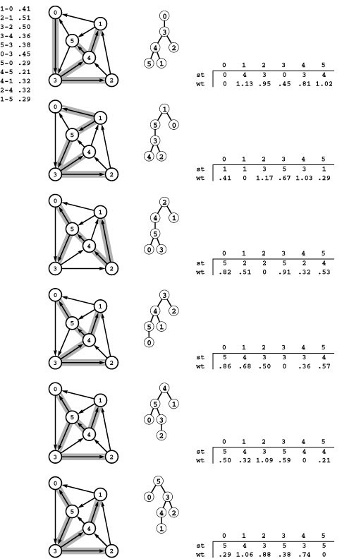
Figure 21.6 Shortest paths trees

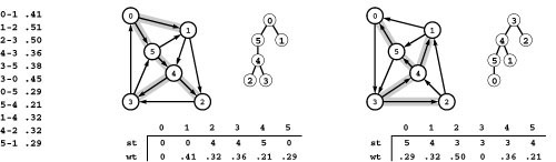
The shortest paths from 0 to the other nodes in this network are 0-1, 0-5-4-2, 0-5-4-3, 0-5-4, and 0-5, respectively. These paths define a spanning tree, which is depicted in three representations (gray edges in the network drawing, oriented tree, and parent links with weights) in the center. Links in the parent-link representation (the one that we typically compute) run in the opposite direction than links in the digraph, so we sometimes work with the reverse digraph. The spanning tree defined by shortest paths from 3 to each of the other nodes in the reverse is depicted on the right. The parent-link representation of this tree gives the shortest paths from each of the other nodes to 2 in the original graph. For example, we can find the shortest path 0-5-4-3 from 0 to 3 by following the links st[0] = 5, st[5] = 4, and st[4] = 3.

the shortest-paths tree, as illustrated in Figure 21.6. We can compute the shortest path from s to t by traveling up the tree from t to s;when we do so, we are traversing edges in the direction opposite from their direction in the network and are visiting the vertices on the path in reverse order (t, st[t], st[st[t]], and so forth).

One way to get the edges on the path in order from source to sink from an SPT is to use a stack. For example, the following code prints a path from the source to a given vertex w:

stack <EDGE *> P; EDGE *e = spt[w];
while (e) { P.push(e); e = spt[e->v()]); }
if (P.empty()) cout << P.top()->v();
while (!P.empty())
    { cout << ’-’ << P.top()->w(); P.pop(); }

In a class implementation, we could use code similar to this to provide clients with a vector that contains the edges of the path.

If we simply want to print or otherwise process the edges on the path, going all the way through the path in reverse order to get to the first edge in this way may be undesirable. One approach to get around this difficulty is to work with the reverse network, as illustrated in Figure 21.6. We use reverse order and edge relaxation in single-source problems because the SPT gives a compact representation of the shortest paths from the source to all the other vertices, in a vector with just V entries.

Next, we consider path relaxation, which is the basis of some of our all-pairs algorithms: Does going through a given vertex lead us to a shorter path that connects two other given vertices? For example, suppose that, for three vertices s, x, and t, we wish to know whether it is better to go from s to x and then from x to t or to go from s to t without going through x. For straight-line connections in a Euclidean space, the triangle inequality tells us that the route through x cannot be shorter than the direct route from s to t, but for paths in a network, it could be (see Figure 21.7). To determine which, we need to know the lengths of paths from s to x, x to t, and of those from s to t (that do not include x). Then, we simply test whether or not the sum of the first two is less than the third; if it is, we update our records accordingly.

Path relaxation is appropriate for all-pairs solutions where we maintain the lengths of the shortest paths that we have encountered between all pairs of vertices. Specifically, in all-pairs–shortest-paths code of this kind, we maintain a vector of vectors d such that d[s][t] is the shortest-path length from s to t, and we also maintain a vector of vectors p such that p[s][t] is the next vertex on a shortest path from s to t. We refer to the former as the distances matrix and the latter as the paths matrix. Figure 21.8 shows the two matrices for our example network. The distances matrix is a prime objective of the computation, and we use the paths matrix because it is clearly more compact than, but carries the same information as, the full list of paths that is illustrated in Figure 21.3.

Figure 21.7 Path relaxation

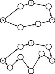
These diagrams illustrate the relaxation operation that underlies our all-pairs shortest-paths algorithms. We keep track of the best known path between all pairs of vertices and ask whether a vertex i is evidence that the shortest known path from s to t could be improved. In the top example, it is not; in the bottom example, it is. Whenever we encounter a vertex i such that the length of the shortest known path from s to i plus the length of the shortest known path from i to t is smaller than the length of the shortest known path from s to t, then we update our data structures to indicate that we now know a shorter path from s to t (head towards i first).

In terms of these data structures, path relaxation amounts to the following code:

if (d[s][t] > d[s][x] + d[x][t])
  { d[s][t] = d[s][x] + d[x][t]; p[s][t] = p[s][x]; }

Like edge relaxation, this code reads as a restatement of the informal description that we have given, so we use it directly in our implementations. More formally, path relaxation reflects the following.

Property 21.1 If a vertex x is on a shortest path from s to t, then that path consists of a shortest path from s to x followed by a shortest path from x to t.

Proof: By contradiction. We could use any shorter path from s to x or from x to t to build a shorter path from s to t.

We encountered the path-relaxation operation when we discussed transitive-closure algorithms, in Section 19.3. If the edge and path weights are either 1 or infinite (that is, a path’s weight is 1 only if all that path’s edges have weight 1), then path relaxation is the operation that we used in Warshall’s algorithm (if we have a path from s to x and a path from x to t, then we have a path from s to t). If we define a path’s weight to be the number of edges on that path, then

Figure 21.8 All shortest paths

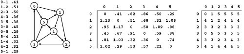
The two matrices on the right are compact representations of all the shortest paths in the sample network on the left, containing the same information in the exhaustive list in Figure 21.3. The distances matrix on the left contains the shortest-path length: The entry in row s and column t is the length of the shortest path from s to t. The paths matrix on the right contains the information needed to execute the path: The entry in row s and column t is the next vertex on the path from s to t.

Warshall’s algorithm generalizes to Floyd’s algorithm for finding all shortest paths in unweighted digraphs; it further generalizes to apply to networks, as we see in Section 21.3.

From a mathematician’s perspective, it is important to note that these algorithms all can be cast in a general algebraic setting that unifies and helps us to understand them. From a programmer’s perspective, it is important to note that we can implement each of these algorithms using an abstract + operator (to compute path weights from edge weights) and an abstract < operator (to compute the minimum value in a set of path weights), both solely in the context of the relaxation operation (see Exercises 19.55 and 19.56).

Property 21.1 implies that a shortest path from s to t contains shortest paths from s to every other vertex along the path to t. Most shortest-paths algorithms also compute shortest paths from s to every vertex that is closer to s than to t (whether or not the vertex is on the path from s to t), although that is not a requirement (see Exercise 21.18). Solving the source–sink shortest-paths problem with such an algorithm when t is the vertex that is farthest from s is equivalent to solving the single-source shortest-paths problem for s. Conversely, we could use a solution to the single-source shortest-paths problem from s as a method for finding the vertex that is farthest from s.

The paths matrix that we use in our implementations for the all-pairs problem is also a representation of the shortest-paths trees for each of the vertices. We defined p[s][t] to be the vertex that follows s on a shortest path from s to t. It is thus the same as the vertex that precedes s on the shortest path from t to s in the reverse network. In other words, column t in the paths matrix of a network is a vertex-indexed vector that represents the SPT for vertex t in its reverse. Conversely, we can build the paths matrix for a network by

Figure 21.9 All shortest paths in a network

These diagrams depict the SPTs for each vertex in the reverse of the network in Figure 21.8 (0 to 5, top to bottom), as network subtrees (left), oriented trees (center), and parent-link representation including a vertex-indexed array for path length (right). Putting the arrays together to form path and distance matrices (where each array becomes a column) gives the solution to the all-pairs shortest-paths problem illustrated in Figure 21.8.

filling each column with the vertex-indexed vector representation of the SPT for the appropriate vertex in the reverse. This correspondence is illustrated in Figure 21.9.

In summary, relaxation gives us the basic abstract operations that we need to build our shortest paths algorithms. The primary complication is the choice of whether to provide the first or final edge on the shortest path. For example, single-source algorithms are more naturally expressed by providing the final edge on the path so that we need only a single vertex-indexed vector to reconstruct the path, since all paths lead back to the source. This choice does not present a fundamental difficulty because we can either use the reverse graph as warranted or provide member functions that hide this difference from clients. For example, we could specify a member function in the interface that returns the edges on the shortest path in a vector (see Exercises 21.15 and 21.16).

Accordingly, for simplicity, all of our implementations in this chapter include a member function dist that returns a shortest-path length and either a member function path that returns the first edge on a shortest path or a member function pathR that returns the final edge on a shortest path. For example, our single-source implementations that use edge relaxation typically implement these functions as follows:

Edge *pathR(int w) const { return spt[w]; }
double dist(int v) { return wt[v]; }

Similarly, our all-paths implementations that use path relaxation typically implement these functions as follows:

Edge *path(int s, int t) { return p[s][t]; }
double dist(int s, int t) { return d[s][t]; }

In some situations, it might be worthwhile to build interfaces that standardize on one or the other or both of these options; we choose the most natural one for the algorithm at hand.

Exercises

• 21.12 Draw the SPT from 0 for the network defined in Exercise 21.1 and for its reverse. Give the parent-link representation of both trees.

21.13 Consider the edges in the network defined in Exercise 21.1 to be undirected edges such that each edge corresponds to equal-weight edges in both directions in the network. Answer Exercise 21.12 for this corresponding network.

• 21.14 Change the direction of edge 0-2 in Figure 21.2. Draw two different SPTs that are rooted at 2 for this modified network.

21.15 Write a function that uses the pathR member function from a single-source implementation to put pointers to the edges on the path from the source v to a given vertex w in an STL vector.

21.16 Write a function that uses the path member function from an all-paths implementation to put pointers to the edges on the path from a given vertex v to another given vertex w in an STL vector.

21.17 Write a program that uses your function from Exercise 21.16 to print out all of the paths, in the style of Figure 21.3.

21.18 Give an example that shows how we could know that a path from s to t is shortest without knowing the length of a shorter path from s to x for some x.

21.2 Dijkstra’s Algorithm

In Section 20.3, we discussed Prim’s algorithm for finding the minimum spanning tree (MST) of a weighted undirected graph: We build it one edge at a time, always taking next the shortest edge that connects a vertex on the MST to a vertex not yet on the MST. We can use a nearly identical scheme to compute an SPT. We begin by putting the source on the SPT; then, we build the SPT one edge at a time, always taking next the edge that gives a shortest path from the source to a vertex not on the SPT. In other words, we add vertices to the SPT in order of their distance (through the SPT) to the start vertex. This method is known as Dijkstra’s algorithm.

As usual, we need to make a distinction between the algorithm at the level of abstraction in this informal description and various concrete implementations (such as Program 21.1) that differ primarily in graph representation and priority-queue implementations, even though such a distinction is not always made in the literature. We shall consider other implementations and discuss their relationships with Program 21.1 after establishing that Dijkstra’s algorithm correctly performs the single-source shortest-paths computation.

Property 21.2 Dijkstra’s algorithm solves the single-source shortest-paths problem in networks that have nonnegative weights.

Proof: Given a source vertex s, we have to establish that the tree path from the root s to each vertex x in the tree computed by Dijkstra’s algorithm corresponds to a shortest path in the graph from s to x. This fact follows by induction. Assuming that the subtree so far computed has the property, we need only to prove that adding a new vertex x adds a shortest path to that vertex. But all other paths to x must begin with a tree path followed by an edge to a vertex not on the tree. By construction, all such paths are longer than the one from s to x that is under consideration.

The same argument shows that Dijkstra’s algorithm solves the source–sink shortest-paths problem, if we start at the source and stop when the sink comes off the priority queue.

The proof breaks down if the edge weights could be negative, because it assumes that a path’s length does not decrease when we add more edges to the path. In a network with negative edge weights, this assumption is not valid because any edge that we encounter might lead to some tree vertex and might have a sufficiently large negative weight to give a path to that vertex shorter than the tree path. We consider this defect in Section 21.7 (see Figure 21.28).

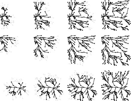
Figure 21.10 shows the evolution of an SPT for a sample graph when computed with Dijkstra’s algorithm; Figure 21.11 shows an oriented drawing of a larger SPT tree. Although Dijkstra’s algorithm differs from Prim’s MST algorithm in only the choice of priority, SPT trees are different in character from MSTs. They are rooted at the start vertex and all edges are directed away from the root, whereas MSTs are unrooted and undirected. We sometimes represent MSTs as directed, rooted trees when we use Prim’s algorithm, but such structures are still different in character from SPTs (compare the oriented drawing in Figure 20.9 with the drawing in Figure 21.11). Indeed, the nature of the SPT somewhat depends on the choice of start vertex as well, as depicted in Figure 21.12.

Dijkstra’s original implementation, which is suitable for dense graphs, is precisely like Prim’s MST algorithm. Specifically, we simply change the assignment of the priority P in Program 20.6 from

  P = e->wt()

(the edge weight) to

  P = wt[v] + e->wt()

(the distance from the source to the edge’s destination). This change gives the classical implementation of Dijkstra’s algorithm: We grow

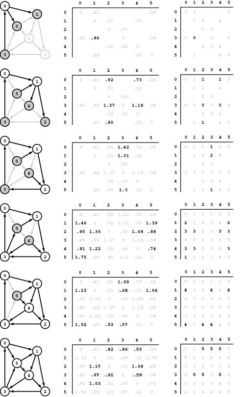
Figure 21.10 Dijkstra’s algorithm

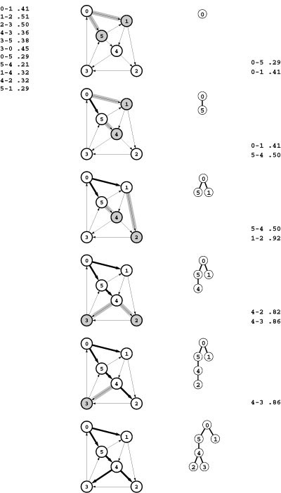
This sequence depicts the construction of a shortest-paths spanning tree rooted at vertex 0 by Dijkstra’s algorithm for a sample network. Thick black edges in the network diagrams are tree edges, and thick gray edges are fringe edges. Oriented drawings of the tree as it grows are shown in the center, and a list of fringe edges is given on the right.

The first step is to add 0 to the tree and the edges leaving it, 0-1 and 0-5, to the fringe (top). Second, we move the shortest of those edges, 0-5, from the fringe to the tree and check the edges leaving it: The edge 5-4 is added to the fringe and the edge 5-1 is discarded because it is not part of a shorter path from 0 to 1 than the known path 0-1 (second from top). The priority of 5-4 on the fringe is the length of the path from 0 that it represents, 0-5-4. Third, we move 0-1 from the fringe to the tree, add 1-2 to the fringe, and discard 1-4 (third from top). Fourth, we move 5-4 from the fringe to the tree, add 4-3 to the fringe, and replace 1-2 with 4-2 because 0-5-4-2 is a shorter path than 0-1-2 (fourth from top). We keep at most one edge to any vertex on the fringe, choosing the one on the shortest path from 0. We complete the computation by moving 4-2 and then 4-3 from the fringe to the tree (bottom).

Figure 21.11 Shortest-paths spanning tree

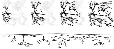
This figure illustrates the progress of Dijkstra’s algorithm in solving the single-source shortest-paths problem in a random Euclidean near-neighbor digraph (with directed edges in both directions corresponding to each line drawn), in the same style as Figures 18.13, 18.24, and 20.9. The search tree is similar in character to BFS because vertices tend to be connected to one another by short paths, but it is slightly deeper and less broad because distances lead to slightly longer paths than path lengths.

an SPT one edge at a time, each time updating the distance to the tree of all vertices adjacent to its destination while at the same time checking all the nontree vertices to find an edge to move to the tree whose destination vertex is a nontree vertex of minimal distance from the source.

Property 21.3 With Dijkstra’s algorithm, we can find any SPT in a dense network in linear time.

Proof: As for Prim’s MST algorithm, it is immediately clear, from inspection of the code of Program 20.6, that the running time is proportional to V², which is linear for dense graphs.

For sparse graphs, we can do better, by viewing Dijkstra’s algorithm as a generalized graph-searching method that differs from depth-first search (DFS), from breadth-first search (BFS), and from Prim’s MST algorithm in only the rule used to add edges to the tree. As in Chapter 20, we keep edges that connect tree vertices to non-tree vertices on a generalized queue called the fringe, use a priority queue to implement the generalized queue, and provide for updating priorities so as to encompass DFS, BFS, and Prim’s algorithm in a single implementation (see Section 20.3). This priority-first search (PFS) scheme also encompasses Dijkstra’s algorithm. That is, changing the assignment of P in Program 20.7 to

P = wt[v] + e->wt()

(the distance from the source to the edge’s destination) gives an implementation of Dijkstra’s algorithm that is suitable for sparse graphs.

Program 21.1 is an alternative PFS implementation for sparse graphs that is slightly simpler than Program 20.7 and that directly matches the informal description of Dijkstra’s algorithm given at the beginning of this section. It differs from Program 20.7 in that it initializes the priority queue with all the vertices in the network and maintains the queue with the aid of a sentinel value for those vertices that are neither on the tree nor on the fringe (unseen vertices with sentinel values); in contrast, Program 20.7 keeps on the priority queue only those vertices that are reachable by a single edge from the tree. Keeping all the vertices on the queue simplifies the code but can incur a small performance penalty for some graphs (see Exercise 21.31).

The general results that we considered concerning the performance of priority-first search (PFS) in Chapter 20 give us specific information about the performance of these implementations of Dijkstra’s algorithm for sparse graphs (Program 21.1 and Program 20.7, suitably modified). For reference, we restate those results in the present context. Since the proofs do not depend on the priority function, they apply without modification. They are worst-case results that apply to both programs, although Program 20.7 may be more efficient for many classes of graphs because it maintains a smaller fringe.

Property 21.4 For all networks and all priority functions, we can compute a spanning tree with PFS in time proportional to the time required for V insert , V delete the minimum , and E decrease key operations in a priority queue of size at most V.

Proof: This fact is immediate from the priority-queue–based implementations in Program 20.7 or Program 21.1. It represents a conservative upper bound because the size of the priority queue is often much smaller than V, particularly for Program 20.7.

Property 21.5 With a PFS implementation of Dijkstra’s algorithm that uses a heap for the priority-queue implementation, we can compute any SPT in time proportional to E lg V.

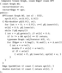
Figure 21.12 SPT examples

These three examples show growing SPTs for three different source locations: left edge (top), upper left corner (center), and center (bottom).

Proof: This result is a direct consequence of Property 21.4.

Property 21.6 Given a graph with V vertices and E edges, let d denote the density E/V. If d < 2, then the running time of Dijkstra’s algorithm is proportional to V lg V. Otherwise, we can improve the worst-case running time by a factor of lg(E/V), to O (E lg_d V ) (which is linear if E is at least V^1+ε)by using a E/V -ary heap for the priority queue.

Proof: This result directly mirrors Property 20.12 and the multiway-heap priority-queue implementation discussed directly thereafter.

Table 21.1 Priority-first search algorithms

These four classical graph-processing algorithms all can be implemented with PFS, a generalized priority-queue–based graph search that builds graph spanning trees one edge at a time. Details of search dynamics depend upon graph representation, priority-queue implementation, and PFS implementation; but the search trees generally characterize the various algorithms, as illustrated in the figures referenced in the fourth column.

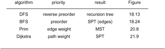
Table 21.1 summarizes pertinent information about the four major PFS algorithms that we have considered. They differ in only the priority function used, but this difference leads to spanning trees that are entirely different from one another in character (as required). For the example in the figures referred to in the table (and for many other graphs), the DFS tree is tall and thin, the BFS tree is short and fat, the SPT is like the BFS tree but neither quite as short nor quite as fat, and the MST is neither short and fat nor tall and thin.

We have also considered four different implementations of PFS. The first is the classical dense-graph implementation that encompasses Dijkstra’s algorithm and Prim’s MST algorithm (Program 20.6); the other three are sparse-graph implementations that differ in priority-queue contents:

• Fringe edges (Program 18.10)

• Fringe vertices (Program 20.7)

• All vertices (Program 21.1)

Of these, the first is primarily of pedagogical value, the second is the most refined of the three, and the third is perhaps the simplest. This framework already describes 16 different implementations of classical graph-search algorithms—when we factor in different priority-queue implementations, the possibilities multiply further. This proliferation

Table 21.2 Cost of implementations of Dijkstra’s algorithm

This table summarizes the cost (worst-case running time) of various implementations of Dijkstra’s algorithm. With appropriate priority-queue implementations, the algorithm runs in linear time (time proportional to V² for dense networks, E for sparse networks), except for networks that are extremely sparse.

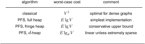
of networks, algorithms, and implementations underscores the utility of the general statements about performance in Properties 21.4 through 21.6, which are also summarized in Table 21.2.

As is true of MST algorithms, actual running times of shortest-paths algorithms are likely to be lower than these worst-case time bounds suggest, primarily because most edges do not necessitate decrease key operations. In practice, except for the sparsest of graphs, we regard the running time as being linear.

The name Dijkstra’s algorithm is commonly used to refer both to the abstract method of building an SPT by adding vertices in order of their distance from the source and to its implementation as the V² algorithm for the adjacency-matrix representation, because Dijkstra presented both in his 1959 paper (and also showed that the same approach could compute the MST). Performance improvements for sparse graphs are dependent on later improvements in ADT technology and priority-queue implementations that are not specific to the shortest-paths problem. Improved performance of Dijkstra’s algorithm is one of the most important applications of that technology (see reference section). As with MSTs, we use terminology such as the “PFS implementation of Dijkstra’s algorithm using d -heaps” to identify specific combinations.

We saw in Section 18.8 that, in unweighted undirected graphs, using preorder numbering for priorities causes the priority queue to operate as a FIFO queue and leads to a BFS. Dijkstra’s algorithm gives us another realization of BFS: When all edge weights are 1, it visits vertices in order of the number of edges on the shortest path to the start vertex. The priority queue does not operate precisely as a FIFO queue would in this case, because items with equal priority do not necessarily come out in the order in which they went in.

Each of these implementations puts the edges of an SPT from vertex 0 in the vertex-indexed vector spt, with the shortest-path length to each vertex in the SPT in the vertex-indexed vector wt and provides member functions that gives clients access to this data. As usual, we can build various graph-processing functions and classes around this basic data (see Exercises 21.21 through 21.28).

Exercises

• 21.19 Show, in the style of Figure 21.10, the result of using Dijkstra’s algorithm to compute the SPT of the network defined in Exercise 21.1 with start vertex 0.

• 21.20 How would you find a second shortest path from s to t in a network?

21.21 Write a client function that uses an SPT object to find the most distant vertex from a given vertex s (the vertex whose shortest path from s is the longest).

21.22 Write a client function that uses an SPT object to compute the average of the lengths of the shortest paths from a given vertex to each of the vertices reachable from it.

21.23 Develop a class based on Program 21.1 with a path member function that returns an STL vector containing pointers to the edges on the shortest path connecting s and t in order from s to t on an STL vector.

• 21.24 Write a client function that uses your class from Exercise 21.23 to print the shortest paths from a given vertex to each of the other vertices in a given network.

21.25 Write a client function that uses an SPT object to find all vertices within a given distance d of a given vertex in a given network. The running time of your function should be proportional to the size of the subgraph induced by those vertices and the vertices incident on them.

21.26 Develop an algorithm for finding an edge whose removal causes maximal increase in the shortest-path length from one given vertex to another given vertex in a given network.

• 21.27 Implement a class that uses SPT objects to perform a sensitivity analysis on the network’s edges with respect to a given pair of vertices s and t: Compute a V-by-V matrix such that, for every u and v, the entry in row u and column v is 1 if u-v is an edge in the network whose weight can be increased without the shortest-path length from s to t being increased and is 0 otherwise.

• 21.28 Implement a class that uses SPT objects to find a shortest path connecting one given set of vertices with another given set of vertices in a given network.

21.29 Use your solution from Exercise 21.28 to implement a client function that finds a shortest path from the left edge to the right edge in a random grid network (see Exercise 20.17).

21.30 Show that an MST of an undirected graph is equivalent to a bottleneck SPT of the graph: For every pair of vertices v and w, it gives the path connecting them whose longest edge is as short as possible.

21.31 Run empirical studies to compare the performance of the two versions of Dijkstra’s algorithm for the sparse graphs that are described in this section (Program 21.1 and Program 20.7, with suitable priority definition), for various networks (see Exercises 21.4–8). Use a standard-heap priority-queue implementation.

21.32 Run empirical studies to learn the best value of d when using a d-heap priority-queue implementation (see Program 20.10) for each of the three PFS implementations that we have discussed (Program 18.10, Program 20.7 and Program 21.1), for various networks (see Exercises 21.4–8).

• 21.33 Run empirical studies to determine the effect of using an index-heap-tournament priority-queue implementation (see Exercise 9.53) in Program 21.1, for various networks (see Exercises 21.4–8).

• 21.34 Run empirical studies to analyze height and average path length in SPTs, for various networks (see Exercises 21.4–8).

21.35 Develop a class for the source–sink shortest-paths problem that is based on code like Program 21.1 but that initializes the priority queue with both the source and the sink. Doing so leads to the growth of an SPT from each vertex; your main task is to decide precisely what to do when the two SPTs collide.

• 21.36 Describe a family of graphs with V vertices and E edges for which the worst-case running time of Dijkstra’s algorithm is achieved.

• 21.37 Develop a reasonable generator for random graphs with V vertices and E edges for which the running time of the heap-based PFS implementation of Dijkstra’s algorithm is superlinear.

• 21.38 Write a client program that does dynamic graphical animations of Dijkstra’s algorithm. Your program should produce images like Figure 21.11 (see Exercises 17.56 through 17.60). Test your program on random Euclidean networks (see Exercise 21.9).

21.3 All-Pairs Shortest Paths

In this section, we consider two classes that solve the all-pairs shortest-paths problem. The algorithms that we implement directly generalize two basic algorithms that we considered in Section 19.3 for the transitive-closure problem. The first method is to run Dijkstra’s algorithm from each vertex to get the shortest paths from that vertex to each of the others. If we implement the priority queue with a heap, the worst-case running time for this approach is proportional to V E lg V, and we can improve this bound to V E for many types of networks by using a d-ary heap. The second method, which allows us to solve the problem directly in time proportional to V³, is an extension of Warshall’s algorithm that is known as Floyd’s algorithm.

Both of these classes implement an abstract–shortest-paths ADT interface for finding shortest distances and paths. This interface, which is shown in Program 21.2, is a generalization to weighted digraphs of the abstract–transitive-closure interface for connectivity queries in digraphs that we studied in Chapter 19. In both class implementations, the constructor solves the all-pairs shortest-paths problem and saves the result in private data members to support query functions that return the shortest-path length from one given vertex to another and either the first or last edge on the path. Implementing such an ADT is a primary reason to use all-pairs shortest-paths algorithms in practice.

Program 21.3 is a sample client program that uses the all– shortest-paths ADT interface to find the weighted diameter of a network. It checks all pairs of vertices to find the one for which the shortest-path length is longest; then, it traverses the path, edge by edge. Figure 21.13 shows the path computed by this program for our Euclidean network example.

Figure 21.13 Diameter of a network

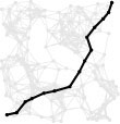
The largest entry in a network’s all-shortest-paths matrix is the diameter of the network: the length of the longest of the shortest paths, depicted here for our sample Euclidean network.

The goal of the algorithms in this section is to support constant-time implementations of the query functions. Typically, we expect to have a huge number of such requests, so we are willing to invest substantial resources in private data members and preprocessing in the constructor to be able to answer the queries quickly. Both of the algorithms that we consider use space proportional to V² for the private data members.

The primary disadvantage of this general approach is that, for a huge network, we may not have so much space available (or we might

not be able to afford the requisite preprocessing time). In principle, our interface provides us with the latitude to trade off preprocessing time and space for query time. If we expect only a few queries, we can do no preprocessing and simply run a single-source algorithm for each query, but intermediate situations require more advanced algorithms (see Exercises 21.48 through 21.50). This problem generalizes one that challenged us for much of Chapter 19: the problem of supporting fast reachability queries in limited space.

The first all-pairs shortest-paths ADT function implementation that we consider solves the problem by using Dijkstra’s algorithm to solve the single-source problem for each vertex. In C++, we can express the method directly, as shown in Program 21.4: We build a vector of SPT objects, one to solve the single-source problem for each vertex. This method generalizes the BFS-based method for unweighted undirected graphs that we considered in Section 17.7. It is also similar

to our use of a DFS that starts at each vertex to compute the transitive closure of unweighted digraphs, in Program 19.4.

Property 21.7 With Dijkstra’s algorithm, we can find all shortest paths in a network that has nonnegative weights in time proportional to V E log_d V, where d = 2if E < 2V, and d =E/V otherwise.

Proof: Immediate from Property 21.6.

As are our bounds for the single-source shortest-paths and the MST problems, this bound is conservative; and a running time of V E is likely for typical graphs.

To compare this implementation with others, it is useful to study the matrices implicit in the vector-of-vectors structure of the private data members. The wt vectors form precisely the distances matrix that we considered in Section 21.1: The entry in row s and column t is the length of the shortest path from s to t. As illustrated in Figures 21.8 and 21.9, the spt vectors from the transpose of the paths matrix: The entry in row s and column t is the last entry on the shortest path from s to t.

For dense graphs, we could use an adjacency-matrix representation and avoid computing the reverse graph by implicitly transposing the matrix (interchanging the row and column indices), as in Program 19.7. Developing an implementation along these lines is an interesting programming exercise and leads to a compact implementation (see Exercise 21.43); however, a different approach, which we consider next, admits an even more compact implementation.

The method of choice for solving the all-pairs shortest-paths problem in dense graphs, which was developed by R. Floyd, is precisely the same as Warshall’s method, except that instead of using the logical or operation to keep track of the existence of paths, it checks distances for each edge to determine whether that edge is part of a new shorter path. Indeed, as we have noted, Floyd’s and Warshall’s algorithms are identical in the proper abstract setting (see Sections 19.3 and 21.1).

Program 21.5 is an all-pairs shortest-paths ADT function that implements Floyd’s algorithm. It explictly uses the matrices from Section 21.1 as private data members: a V -by-V vector of vectors d for the distances matrix, and another V -by-V vector of vectors p for the paths table. For every pair of vertices s and t, the constructor sets

d[s][t] to the shortest-path length from s to t (to be returned by the dist member function) and p[s][t] to the index of the next vertex on the shortest path from s to t (to be returned by the path member function). The implementation is based upon the path relaxation operation that we considered in Section 21.1.

Property 21.8With Floyd’s algorithm, we can find all shortest paths in a network in time proportional to V³.

Proof: The running time is immediate from inspection of the code. We prove that the algorithm is correct by induction in precisely the same way as we did for Warshall’s algorithm. The ith iteration of the loop computes a shortest path from s to t in the network that does not include any vertices with indices greater than i (except possibly the endpoints s and t). Assuming this fact to be true for the ith iteration of the loop, we prove it to be true for the (i+1)st iteration of the loop. A shortest path from s to t that does not include any vertices with indices greater than i+1 is either (i) a path from s to t that does not include any vertices with indices greater than i, of length d[s][t], that was found on a previous iteration of the loop, by the inductive hypothesis; or (ii) comprising a path from s to i and a path from i to t, neither of which includes any vertices with indices greater than i, in which case the inner loop sets d[s][t].

Figure 21.14 is a detailed trace of Floyd’s algorithm on our sample network. If we convert each blank entry to 0 (to indicate the absence of an edge) and convert each nonblank entry to 1 (to indicate the presence of an edge), then these matrices describe the operation of Warshall’s algorithm in precisely the same manner as we did in Figure 19.15. For Floyd’s algorithm, the nonblank entries indicate more than the existence of a path; they give information about the shortest known path. An entry in the distance matrix has the length of the shortest known path connecting the vertices corresponding to the given row and column; the corresponding entry in the paths matrix gives the next vertex on that path. As the matrices become filled with nonblank entries, running Warshall’s algorithm amounts to just double-checking that new paths connect pairs of vertices already known to be connected by a path; in contrast, Floyd’s algorithm must compare (and update if necessary) each new path to see whether the new path leads to shorter paths.

Figure 21.14 Floyd’s algorithm

This sequence shows the construction of the all-pairs shortest-paths matrices with Floyd’s algorithm. For i from 0 to 5 (top to bottom), we consider, for all s and t, all of the paths from s to t having no intermediate vertices greater than i (the shaded vertices). Initially, the only such paths are the network’s edges, so the distances matrix (center) is the graph’s adjacency matrix and the paths matrix (right) is set with p[s][t] = t for each edge s-t. For vertex 0 (top), the algorithm finds that 3-0-1 is shorter than the sentinel value that is present because there is no edge 3-1 and updates the matrices accordingly. It does not do so for paths such as 3-0-5, which is not shorter than the known path 3-5. Next the algorithm considers paths through 0 and 1 (second from top) and finds the new shorter paths 0-1-2, 0-1-4, 3-0-1-2, 3-0-1-4, and 5-1-2. The third row from the top shows the updates corresponding to shorter paths through 0, 1, and 2 and so forth.

Black numbers overstriking gray ones in the matrices indicate situations where the algorithm finds a shorter path than one it found earlier. For example, .91 overstrikes 1.37 in row 3 and column 2 in the bottom diagram because the algorithm discovered that 3-5-4-2 is shorter than 3-0-1-2.

Comparing the worst-case bounds on the running times of Dijkstra’s and Floyd’s algorithms, we can draw the same conclusion for these all-pairs shortest-paths algorithms as we did for the corresponding transitive-closure algorithms in Section 19.3. Running Dijkstra’s algorithm on each vertex is clearly the method of choice for sparse networks, because the running time is close to V E. As density increases, Floyd’s algorithm—which always takes time proportional to V³—becomes competitive (see Exercise 21.67); it is widely used because it is so simple to implement.

A more fundamental distinction between the algorithms, which we examine in detail in Section 21.7, is that Floyd’s algorithm is effective in even those networks that have negative weights (provided that there are no negative cycles). As we noted in Section 21.2, Dijkstra’s method does not necessarily find shortest paths in such graphs.

The classical solutions to the all-pairs shortest-paths problem that we have described presume that we have space available to hold the distances and paths matrices. Huge sparse graphs, where we cannot afford to have any V-by-V matrices, present another set of challenging and interesting problems. As we saw in Chapter 19, it is an open problem to reduce this space cost to be proportional to V while still supporting constant-time shortest-path-length queries. We found the analogous problem to be difficult even for the simpler reachability problem (where we are satisfied with learning in constant time whether there is any path connecting a given pair of vertices), so we cannot expect a simple solution for the all-pairs shortest-paths problem. Indeed, the number of different shortest path lengths is, in general, proportional to V² even for sparse graphs. That value, in some sense, measures the amount of information that we need to process, and perhaps indicates that when we do have restrictions on space, we must expect to spend more time on each query (see Exercises 21.48 through 21.50).

Exercises

• 21.39 Estimate, to within a factor of 10, the largest graph (measured by its number of vertices) that your computer and programming system could handle if you were to use Floyd’s algorithm to compute all its shortest paths in 10 seconds.

• 21.40 Estimate, to within a factor of 10, the largest graph of density 10 (measured by its number of edges) that your computer and programming system could handle if you were to use Dijkstra’s algorithm to compute all its shortest paths in 10 seconds.

21.41 Show, in the style of Figure 21.9, the result of using Dijkstra’s algorithm to compute all shortest paths of the network defined in Exercise 21.1.

21.42 Show, in the style of Figure 21.14, the result of using Floyd’s algorithm to compute all shortest paths of the network defined in Exercise 21.1.

• 21.43 Combine Program 20.6 and Program 21.4 to make an implementation of the all-pairs shortest-paths ADT interface (based on Dijkstra’s algorithm) for dense networks that supports path queries but does not explicitly compute the reverse network. Do not define a separate function for the single-source solution—put the code from Program 20.6 directly in the inner loop and put results directly in private data members d and p like those in Program 21.5).

21.44 Run empirical tests, in the style of Table 20.2, to compare Dijkstra’s algorithm (Program 21.4 and Exercise 21.43) and Floyd’s algorithm (Pro-gram 21.5), for various networks (see Exercises 21.4–8).

21.45 Run empirical tests to determine the number of times that Floyd’s and Dijkstra’s algorithms update the values in the distances matrix, for various networks (see Exercises 21.4–8).

21.46 Give a matrix in which the entry in row s and column t is equal to the number of different simple directed paths connecting s and t in Figure 21.1.

21.47 Implement a class whose constructor computes the path-count matrix that is described in Exercise 21.46 so that it can provide count queries through a public member function in constant time.

• 21.48 Develop a class implementation of the abstract–shortest-paths ADT for sparse graphs that cuts the space cost to be proportional to V, by increasing the query time to be proportional to V.

• 21.49 Develop a class implementation of the abstract–shortest-paths ADT for sparse graphs that uses substantially less than O (V²) space but supports queries in substantially less than O (V ) time. Hint: Compute all shortest paths for a subset of the vertices.

• 21.50 Develop a class implementation of the abstract–shortest-paths ADT for sparse graphs that uses substantially less than O (V²) space and (using randomization) supports queries in constant expected time.

• 21.51 Develop a class implementation of the abstract–shortest-paths ADT that takes the lazy approach of using Dijkstra’s algorithm to build the SPT (and associated distance vector) for each vertex s the first time that the client issues a shortest-path query from s, then references the information on subsequent queries.

21.52 Modify the shortest-paths ADT and Dijkstra’s algorithm to handle shortest-paths computations in networks that have weights on both vertices and edges. Do not rebuild the graph representation (the method described in Exercise 21.4); modify the code instead.

• 21.53 Build a small model of airline routes and connection times, perhaps based upon some flights that you have taken. Use your solution to Exercise 21.52 to compute the fastest way to get from one of the served destinations to another. Then test your program on real data (see Exercise 21.5).

21.4 Shortest Paths in Acyclic Networks

In Chapter 19, we found that, despite our intuition that DAGs should be easier to process than general digraphs, developing algorithms with substantially better performance for DAGs than for general digraphs is an elusive goal. For shortest-paths problems, we do have algorithms for DAGs that are simpler and faster than the priority-queue–based methods that we have considered for general digraphs. Specifically, in this section we consider algorithms for acyclic networks that

• Solve the single-source problem in linear time.

• Solve the all-pairs problem in time proportional to V E.

• Solve other problems, such as finding longest paths.

In the first two cases, we cut the logarithmic factor from the running time that is present in our best algorithms for sparse networks; in the third case, we have simple algorithms for problems that are intractable for general networks. These algorithms are all straightforward extensions to the algorithms for reachability and transitive closure in DAGs that we considered in Chapter 19.

Since there are no cycles at all, there are no negative cycles; so negative weights present no difficulty in shortest-paths problems on DAGs. Accordingly, we place no restrictions on edge-weight values throughout this section.

Next, a note about terminology: We might choose to refer to directed graphs with weights on the edges and no cycles either as weighted DAGs or as acyclic networks. We use both terms interchangeably to emphasize their equivalence and to avoid confusion when we refer to the literature, where both are widely used. It is sometimes convenient to use the former to emphasize differences from unweighted DAGs that are implied by weights and the latter to emphasize differences from general networks that are implied by acyclicity.

The four basic ideas that we applied to derive efficient algorithms for unweighted DAGs in Chapter 19 are even more effective for weighted DAGs.

• Use DFS to solve the single-source problem.

• Use a source queue to solve the single-source problem.

• Invoke either method, once for each vertex, to solve the all-pairs problem.

• Use a single DFS (with dynamic programming) to solve the all-pairs problem.

These methods solve the single-source problem in time proportional to E and the all-pairs problem in time proportional to V E. They are all effective because of topological ordering, which allows us compute shortest paths for each vertex without having to revisit any decisions. We consider one implementation for each problem in this section; we leave the others for exercises (see Exercises 21.62 through 21.65).

We begin with a slight twist. Every DAG has at least one source but could have several, so it is natural to consider the following shortest-paths problem.

Multisource shortest paths Given a set of start vertices, find, for each other vertex w, a shortest path among the shortest paths from each start vertex to w.

This problem is essentially equivalent to the single-source shortest-paths problem. We can convert a multisource problem into a single-source problem by adding a dummy source vertex with zero-length edges to each source in the network. Conversely, we can convert a single-source problem to a multisource problem by working with the induced subnetwork defined by all the vertices and edges reachable from the source. We rarely construct such subnetworks explicitly, because our algorithms automatically process them if we treat the start vertex as though it were the only source in the network (even when it is not).

Topological sorting immediately presents a solution to the multi-source shortest-paths problem and to numerous other problems. We maintain a vertex-indexed vector wt that gives the weight of the shortest known path from any source to each vertex. To solve the multisource shortest-paths problem, we initialize the wt vector to 0 for sources and a large sentinel value for all the other vertices. Then, we process the vertices in topological order. To process a vertex v, we perform a relaxation operation for each outgoing edge v-w that updates the shortest path to w if v-w gives a shorter path from a source to w (through v). This process checks all paths from any source to each vertex in the graph; the relaxation operation keeps track of the minimum-length such path, and the topological sort ensures that we process the vertices in an appropriate order.

We can implement this method directly in one of two ways. The first is to add a few lines of code to the topological sort code in Program 19.8: Just after we remove a vertex v from the source queue, we perform the indicated relaxation operation for each of its edges (see Exercise 21.56). The second is to put the vertices in topological order, then to scan through them and to perform the relaxation operations precisely as described in the previous paragraph.

These same processes (with other relaxation operations) can solve many graph-processing problems. For example, Program 21.6 is an implementation of the second approach (sort, then scan) for solving the multisource longest-paths problem: For each vertex in the network, what is a longest path from some source to that vertex? We interpret the wt entry associated with each vertex to be the length of the longest known path from any source to that vertex, initialize all of the weights to 0, and change the sense of the comparison in the relaxation operation. Figure 21.15 traces the operation of Program 21.6 on a sample acyclic network.

Property 21.9We can solve the multisource shortest-paths problem and the multisource longest-paths problem in acyclic networks in linear time.

Proof: The same proof holds for longest path, shortest path, and many other path properties. To match Program 21.6, we state the proof for longest paths. We show by induction on the loop variable i that, for all vertices v = ts[j] with j < i that have been processed, wt[v] is the length of the longest path from a source to v. When v = ts[i], let t be the vertex preceding v on any path from a source to v. Since vertices in the ts vector are in topologically sorted order, t must have been processed already. By the induction hypothesis, wt[t] is the length of the longest path to t, and the relaxation step in the code checks whether that path gives a longer path to v through t. The induction hypothesis also implies that all paths to v are checked in this way as v is processed.

This property is significant because it tells us that processing acyclic networks is considerably easier than processing networks that

Figure 21.15 Computing longest paths in an acyclic network

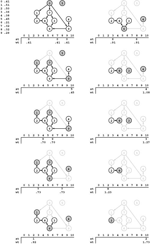
In this network, each edge has the weight associated with the vertex that it leads from, listed at the top left. Sinks have edges to a dummy vertex 10, which is not shown in the drawings. The wt array contains the length of the longest known path to each vertex from some source, and the st array contains the previous vertex on the longest path. This figure illustrates the operation of Program 21.6, which picks from among the sources (the shaded nodes in each diagram) using the FIFO discipline, though any of the sources could be chosen at each step. We begin by removing 0 and checking each of its incident edges, discovering one-edge paths of length .41 to 1, 7, and 9. Next, we remove 5 and record the one-edge path from 5 to 10 (left, second from top). Next, we remove 9 and record the paths 0-9-4 and 0-9-6, of length .70 (left, third from top). We continue in this way, changing the arrays whenever we find longer paths. For example, when we remove 7 (left, second from bottom) we record paths of length .73 to 8 and 3; then, later, when we remove 6, we record longer paths (of length .91) to 8 and 3 (right, top). The point of the computation is to find the longest path to the dummy node 10. In this case, the result is the path 0-9-6-8-2, of length 1.73.

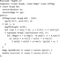
have cycles. For shortest paths, the method is faster than Dijkstra’s algorithm by a factor proportional to the cost of the priority-queue operations in Dijkstra’s algorithm. For longest paths, we have a linear algorithm for acyclic networks but an intractable problem for general networks. Moreover, negative weights present no special difficulty here, but they present formidable barriers for algorithms on general networks, as discussed in Section 21.7.

The method just described depends on only the fact that we process the vertices in topological order. Therefore, any topological-sorting

Figure 21.16 Shortest paths in an acyclic network

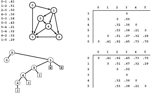
This diagram depicts the computation of the all-shortest-distances matrix (bottom right) for a sample weighted DAG (top left), computing each row as the last action in a recursive DFS function. Each row is computed from the rows for adjacent vertices, which appear earlier in the list, because the rows are computed in reverse topological order (postorder traversal of the DFS tree shown at the bottom left). The array on the top right shows the rows of the matrix in the order that they are computed. For example, to compute each entry in the row for 0 we add .41 to the corresponding entry in the row for 1 (to get the distance to it from 0 after taking 0-1), then add .45 to the corresponding entry in the row for 3 (to get the distance to it from 0 after taking 0-3), and take the smaller of the two. The computation is essentially the same as computing the transitive closure of a DAG (see, for example, Figure 19.23). The most significant difference between the two is that the transitive-closure algorithm could ignore down edges (such as 1-2 in this example) because they go to vertices known to be reachable, while the shortest-paths algorithm has to check whether paths associated with down edges are shorter than known paths. If we were to ignore 1-2 in this example, we would miss the shortest paths 0-1-2 and 1-2.

algorithm can be adapted to solve shortest- and longest-paths problems and other problems of this type (see, for example, Exercises 21.56 and 21.62).

As we know from Chapter 19, the DAG abstraction is a general one that arises in many applications. For example, we see an application in Section 21.6 that seems unrelated to networks but that can be addressed directly with Program 21.6.

Next, we turn to the all-pairs shortest-paths problem for acyclic networks. As in Section 19.3, one method that we could use to solve this problem is to run a single-source algorithm for each vertex (see Exercise 21.65). The equally effective approach that we consider here is to use a single DFS with dynamic programming, just as we did for computing the transitive closure of DAGs in Section 19.5 (see Program 19.9). If we consider the vertices at the end of the recursive function, we are processing them in reverse topological order and can derive the shortest-path vector for each vertex from the shortest-path vectors for each adjacent vertex, simply by using each edge in a relaxation step.

Program 21.7 is an implementation along these lines. The operation of this program on a sample weighted DAG is illustrated in Figure 21.16. Beyond the generalization to include relaxation, there is one important difference between this computation and the transitiveclosure

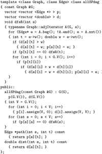
Figure 21.17 All longest paths in an acyclic network

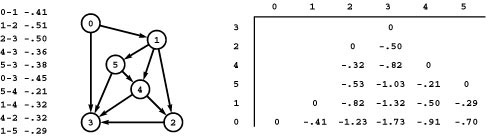
Our method for computing all shortest paths in acyclic networks works even if the weights are negative. Therefore, we can use it to compute longest paths, simply by first negating all the weights, as illustrated here for the network in Figure 21.16. The longest simple path in this network is 0-1-5-4-2-3, of weight 1.73.

computation for DAGs: In Program 19.9, we had the choice of ignoring down edges in the DFS tree because they provide no new information about reachability; in Program 21.7, however, we need to consider all edges, because any edge might lead to a shorter path.

Property 21.10 We can solve the all-pairs shortest-paths problem in acyclic networks with a single DFS in time proportional to V E.

Proof: This fact follows immediately from the strategy of solving the single-source problem for each vertex (see Exercise 21.65). We can also establish it by induction, from Program 21.7. After the recursive calls for a vertex v, we know that we have computed all shortest paths for each vertex on v’s adjacency list, so we can find shortest paths from v to each vertex by checking each of v’s edges. We do V relaxation steps for each edge, for a total of V E relaxation steps.

Thus, for acyclic networks, topological sorting allows us to avoid the cost of the priority queue in Dijkstra’s algorithm. Like Floyd’s algorithm, Program 21.7 also solves problems more general than those solved by Dijkstra’s algorithm, because, unlike Dijkstra’s (see Section 21.7), this algorithm works correctly even in the presence of negative edge weights. If we run the algorithm after negating all the weights in an acyclic network, it finds all longest paths, as depicted in Figure 21.17. Or, we can find longest paths by reversing the inequality test in the relaxation algorithm, as in Program 21.6.

The other algorithms for finding shortest paths in acyclic networks that are mentioned at the beginning of this section generalize the methods from Chapter 19 in a manner similar to the other algorithms that we have examined in this chapter. Developing implementations of them is a worthwhile way to cement your understanding of both DAGs and shortest paths (see Exercises 21.62 through 21.65). All the methods run in time proportional to V E in the worst case, with actual costs dependent on the structure of the DAG. In principle, we might do even better for certain sparse weighted DAGs (see Exercise 19.117).

Exercises

• 21.54 Give the solutions to the multisource shortest- and longest-paths problems for the network defined in Exercise 21.1, with the directions of edges 2-3 and 1-0 reversed.

• 21.55 Modify Program 21.6 such that it solves the multisource shortest-paths problem for acyclic networks.

• 21.56 Implement a class with the same interface as Program 21.6 that is derived from the source-queue–based topological-sorting code of Program 19.8, performing the relaxation operations for each vertex just after that vertex is removed from the source queue.

• 21.57 Define an ADT for the relaxation operation, provide implementations, and modify Program 21.6 to use your ADT such that you can use Program 21.6 to solve the multisource shortest-paths problem, the multisource longest-paths problem, and other problems, just by changing the relaxation implementation.

21.58 Use your generic implementation from Exercise 21.57 to implement a class with member functions that return the length of the longest paths from any source to any other vertex in a DAG, the length of the shortest such path, and the number of vertices reachable via paths whose lengths fall within a given range.

• 21.59 Define properties of relaxation such that you can modify the proof of Property 21.9 to apply an abstract version of Program 21.6 (such as the one described in Exercise 21.57).

• 21.60 Show, in the style of Figure 21.16, the computation of the all-pairs shortest-paths matrices for the network defined in Exercise 21.54 by Program 21.7.

• 21.61 Give an upper bound on the number of edge weights accessed by Program 21.7, as a function of basic structural properties of the network. Write a program to compute this function, and use it to estimate the accuracy of the V E bound, for various acyclic networks (add weights as appropriate to the models in Chapter 19).

• 21.62 Write a DFS-based solution to the multisource shortest-paths problem for acyclic networks. Does your solution work correctly in the presence of negative edge weights? Explain your answer.

• 21.63 Extend your solution to Exercise 21.62 to provide an implementation of the all-pairs shortest-paths ADT interface for acyclic networks that builds the all-paths and all-distances matrices in time proportional to V E.

21.64 Show, in the style of Figure 21.9, the computation of all shortest paths of the network defined in Exercise 21.54 using the DFS-based method of Exercise 21.63.

• 21.65 Modify Program 21.6 such that it solves the single-source shortest-paths problem in acyclic networks, then use it to develop an implementation of the all-pairs shortest-paths ADT interface for acyclic networks that builds the all-paths and all-distances matrices in time proportional to V E.

• 21.66 Work Exercise 21.61 for the DFS-based (Exercise 21.63) and for the topological-sort–based (Exercise 21.65) implementations of the all-pairs shortest-paths ADT. What inferences can you draw about the comparative costs of the three methods?

21.67 Run empirical tests, in the style of Table 20.2, to compare the three class implementations for the all-pairs shortest-paths problem described in this section (see Program 21.7, Exercise 21.63, and Exercise 21.65), for various acyclic networks (add weights as appropriate to the models in Chapter 19).

21.5 Euclidean Networks

In applications where networks model maps, our primary interest is often in finding the best route from one place to another. In this section, we examine a strategy for this problem: a fast algorithm for the source–sink shortest-path problem in Euclidean networks, which are networks whose vertices are points in the plane and whose edge weights are defined by the geometric distances between the points.

These networks satisfy two important properties that do not necessarily hold for general edge weights. First, the distances satisfy the triangle inequality: The distance from s to d is never greater than the distance from s to x plus the distance from x to d. Second, vertex positions give a lower bound on path length: No path from s to d will be shorter than the distance from s to d. The algorithm for the source–sink shortest-paths problem that we examine in this section takes advantage of these two properties to improve performance.

Often, Euclidean networks are also symmetric: Edges run in both directions. As mentioned at the beginning of the chapter, such networks arise immediately if, for example, we interpret the adjacency-matrix or adjacency-lists representation of an undirected weighted Euclidean graph (see Section 20.7) as a weighted digraph (network). When we draw an undirected Euclidean network, we assume this interpretation to avoid proliferation of arrowheads in the drawings.

The basic idea is straightforward: Priority-first search provides us with a general mechanism to search for paths in graphs. With Dijkstra’s algorithm, we examine paths in order of their distance from the start vertex. This ordering ensures that, when we reach the sink, we have examined all paths in the graph that are shorter, none of which took us to the sink. But in a Euclidean graph, we have additional information: If we are looking for a path from a source s to a sink d and we encounter a third vertex v, then we know that not only do we have to take the path that we have found from s to v, but also the best that we could possibly do in traveling from v to d is first to take an edge v-w and then to find a path whose length is the straight-line distance from w to d (see Figure 21.18). With priority-first search, we can easily take into account this extra information to improve performance. We use the standard algorithm, but we use the sum of the following three quantities as the priority of each edge v-w: the length of the known path from s to v, the weight of the edge v-w, and the distance from w to t. If we always pick the edge for which this number is smallest, then, when we reach t, we are still assured that there is no shorter path in the graph from s to t. Furthermore, in typical networks we reach this conclusion after doing far less work than we would were we using Dijkstra’s algorithm.

Figure 21.18 Edge relaxation (Euclidean)

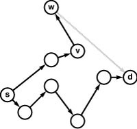
In a Euclidean graph, we can take distances to the destination into account in the relaxation operation as we compute shortest paths. In this example, we could deduce that the path depicted from s to v plus v-w cannot lead to a shorter path from s to d than the one already found because the length of any such path must be at least the length of the path from s to v plus the length of v-w plus the straight-line distance from w to d, which is greater than the length of the known path from s to d. Tests like this one can significantly reduce the number of paths that we have to consider.

To implement this approach, we use a standard PFS implementation of Dijkstra’s algorithm (Program 21.1, since Euclidean graphs are normally sparse, but also see Exercise 21.73) with two changes: First, instead of initializing wt[s] at the beginning of the search to 0.0, we set it to the quantity dist(s, d), where distance is a function that returns the distance between two vertices. Second, we define the priority P to be the function

(wt[v] + e->wt() + distance(w, d) - distance(v, d))

instead of the function (wt[v] + e->wt()) that we used in Program 21.1 (recall that v and w are local variables that are set to the values e->v() and e->w(), respectively. These changes, to which we refer as the Euclidean heuristic, maintain the invariant that the quantity wt[v] - distance(v, d) is the length of the shortest path through the network from s to v, for every tree vertex v (and therefore wt[v] is a lower bound on the length of the shortest possible path through v from s to d). We compute wt[w] by adding to this quantity the edge weight (the distance to w) plus the distance from w to the sink d.

Figure 21.19 Shortest path in a Euclidean graph

When we direct the shortest-path search towards the destination vertex, we can restrict the search to vertices within a relatively small ellipse around the path, as illustrated in these three examples, which show SPT subtrees from the examples in Figure 21.12.

Property 21.11 Priority-first search with the Euclidean heuristic solves the source–sink shortest-paths problem in Euclidean graphs.

Proof: The proof of Property 21.2 applies: At the time that we add a vertex x to the tree, the addition of the distance from x to d to the priority does not affect the reasoning that the tree path from s to x is a shortest path in the graph from s to x, since the same quantity is added to the length of all paths to x. When d is added to the tree, we know that no other path from s to d is shorter than the tree path, because any such path must consist of a tree path followed by an edge to some vertex w that is not on the tree, followed by a path from w to d (whose length cannot be shorter than the distance from w to d); and, by construction, we know that the length of the path from s to w plus the distance from w to d is no smaller than the length of the tree path from s to d.

In Section 21.6, we discuss another simple way to implement the Euclidean heuristic. First, we make a pass through the graph to change the weight of each edge: For each edge v-w, we add the quantity distance(w, d) - distance(v, d). Then, we run a standard shortest-path algorithm, starting at s (with wt[s] initialized to distance(s, d)) and stopping when we reach d. This method is computationally equivalent to the method that we have described (which essentially computes the same weights on the fly) and is a specific example of a basic operation known as reweighting a network. Reweighting plays an essential role in solving the shortest-paths problems with negative weights; we discuss it in detail in Section 21.6.

The Euclidean heuristic affects the performance but not the correctness of Dijkstra’s algorithm for the source–sink shortest-paths computation. As discussed in the proof of Property 21.2, using the standard algorithm to solve the source–sink problem amounts to building an SPT that has all vertices closer to the start than the sink d. With the Euclidean heuristic, the SPT contains just the vertices whose path from s plus distance to d is smaller than the length of the shortest path from s to d. We expect this tree to be substantially smaller for many applications because the heuristic prunes a substantial number of long paths. The precise savings is dependent on the structure of the graph and the geometry of the vertices. Figure 21.19 shows the operation of the Euclidean heuristic on our sample graph, where the savings are substantial. We refer to the method as a heuristic because there is no guarantee that there will be any savings at all: It could always be the case that the only path from source to sink is a long one that wanders arbitrarily far from the source before heading back to the sink (see Exercise 21.80).

Figure 21.20 Euclidean heuristic cost bounds

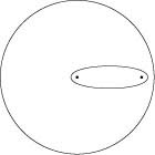
When we direct the shortest-path search towards the destination vertex, we can restrict the search to vertices within an ellipse around the path, as compared to the circle centered at s that is required by Dijkstra’s algorithm. The radius of the circle and the shape of the ellipse are determined by the length of the shortest path.

Figure 21.20 illustrates the basic underlying geometry that describes the intuition behind the Euclidean heuristic: If the shortest-path length from s to d is z, then vertices examined by the algorithm fall roughly within the ellipse defined as the locus of points x for which the distance from s to x plus the distance from x to d is equal to z. For typical Euclidean graphs, we expect the number of vertices in this ellipse to be far smaller than the number of vertices in the circle of radius z that is centered at the source (those that would be examined by Dijkstra’s algorithm).

Precise analysis of the savings is a difficult analytic problem and depends on models of both random point sets and random graphs (see reference section). For typical situations, we expect that, if the standard algorithm examines X vertices in computing a source–sink shortest path, the Euclidean heuristic will cut the cost to be proportional to , which leads to an expected running time proportional to for dense graphs and proportional to pV for sparse graphs. This example illustrates that the difficulty of developing an appropriate model or analyzing associated algorithms should not dissuade us from taking advantage of the substantial savings that are available in many applications, particularly when the implementation (add a term to the priority) is trivial.

The proof of Property 21.11 applies for any function that gives a lower bound on the distance from each vertex to d. Might there be other functions that will cause the algorithm to examine even fewer vertices than the Euclidean heuristic? This question has been studied in a general setting that applies to a broad class of combinatorial search algorithms. Indeed, the Euclidean heuristic is a specific instance of an algorithm called A * (pronounced “ay-star”). This theory tells us that using the best available lower-bound function is optimal; stated another way, the better the bound function, the more efficient the search. In this case, the optimality of A* tells us that the Euclidean heuristic will certainly examine no more vertices than Dijkstra’s algorithm (which is A* with a lower bound of 0). The analytic results just described give more precise information for specific random network models.

We can also use properties of Euclidean networks to help build efficient implementations of the abstract–shortest-paths ADT, trading time for space more effectively than we can for general networks (see Exercises 21.48 through 21.50). Such algorithms are important in applications such as map processing, where networks are huge and sparse. For example, suppose that we want to develop a navigation system based on shortest paths for a map with millions of roads. We perhaps can store the map itself in a small onboard computer, but the distances and paths matrices are much too large to be stored (see Exercises 21.39 and 21.40); therefore, the all-paths algorithms of Section 21.3 are not effective. Dijkstra’s algorithm also may not give sufficiently short response times for huge maps. Exercises 21.77 through 21.78 explore strategies whereby we can invest a reasonable amount of preprocessing and space to provide fast responses to source– sink shortest-paths queries.

Exercises

• 21.68 Find a large Euclidean graph online—perhaps a map with an underlying table of locations and distances between them, telephone connections with costs, or airline routes and rates.

21.69 Using the strategies described in Exercises 17.71 through 17.73, write programs that generate random Euclidean graphs by connecting vertices arranged in a -by- grid.

• 21.70 Show that the partial SPT computed by the Euclidean heuristic is independent of the value that we use to initialize wt[s]. Explain how to compute the shortest-path lengths from the initial value.

• 21.71 Show, in the style of Figure 21.10, what is the result when you use the Euclidean heuristic to compute a shortest path from 0 to 6 in the network defined in Exercise 21.1.

21.72 Describe what happens if the function distance(s, t), used for the Euclidean heuristic, returns the actual shortest-path length from s to t for all pairs of vertices.

21.73 Develop an class implementation for shortest paths in dense Euclidean graphs that is based upon a graph representation that supports the edge function and an implementation of Dijkstra’s algorithm (Program 20.6, with an appropriate priority function).

21.74 Run empirical studies to test the effectiveness of the Euclidean shortest-path heuristic, for various Euclidean networks (see Exercises 21.9, 21.68, 21.69, and 21.80). For each graph, generate V/ 10 random pairs of vertices, and print a table that shows the average distance between the vertices, the average length of the shortest path between the vertices, the average ratio of the number of vertices examined with the Euclidean heuristic to the number of vertices examined with Dijkstra’s algorithm, and the average ratio of the area of the ellipse associated with the Euclidean heuristic with the area of the circle associated with Dijkstra’s algorithm.

21.75 Develop a class implementation for the source-sink shortest-paths problemin Euclidean graphs that is based on the bidirectional search described in Exercise 21.35.

• 21.76 Use a geometric interpretation to provide an estimate of the ratio of the number of vertices in the SPT produced by Dijkstra’s algorithm for the source–sink problem to the number of vertices in the SPTs produced in the two-way version described in Exercise 21.75.

21.77 Develop a class implementation for shortest paths in Euclidean graphs that performs the following preprocessing step in the constructor: Divide the map region into a W -by-W grid, and then use Floyd’s all-pairs shortest-paths algorithm to compute a W²-by-W² matrix, where row i and column j contain the length of a shortest path connecting any vertex in grid square i to any vertex in grid square j. Then, use these shortest-path lengths as lower bounds to improve the Euclidean heuristic. Experiment with a few different values of W such that you expect a small constant number of vertices per grid square.

21.78 Develop an implementation of the all-pairs shortest-paths ADT for Euclidean graphs that combines the ideas in Exercises 21.75 and 21.77.

21.79 Run empirical studies to compare the effectiveness of the heuristics described in Exercises 21.75 through 21.78, for various Euclidean networks (see Exercises 21.9, 21.68, 21.69, and 21.80).

21.80 Expand your empirical studies to include Euclidean graphs that are derived by removal of all vertices and edges from a circle of radius r in the center, for r =0.1, 0.2, 0.3, and 0.4. (These graphs provide a severe test of the Euclidean heuristic.)

21.81 Give a direct implementation of Floyd’s algorithm for an implementation of the network ADT for implicit Euclidean graphs defined by N points in the plane with edges that connect points within d of each other. Do not explicitly represent the graph; rather, given two vertices, compute their distance to determine whether an edge exists and, if one does, what its length is.

21.82 Develop an implementation for the scenario described in Exercise 21.81 that builds a neighbor graph and then uses Dijkstra’s algorithm from each vertex (see Program 21.1).

21.83 Run empirical studies to compare the time and space needed by the algorithms in Exercises 21.81 and 21.82, for d = 0.1, 0.2, 0.3, and 0.4.

• 21.84 Write a client program that does dynamic graphical animations of the Euclidean heuristic. Your program should produce images like Figure 21.19 (see Exercise 21.38). Test your program on various Euclidean networks (see Exercises 21.9, 21.68, 21.69, and 21.80).

21.6 Reduction

It turns out that shortest-paths problems—particularly the general case, where negative weights are allowed (the topic of Section 21.7)—represent a general mathematical model that we can use to solve a variety of other problems that seem unrelated to graph processing. This model is the first among several such general models that we encounter. As we move to more difficult problems and increasingly general models, one of the challenges that we face is to characterize precisely relationships among various problems. Given a new problem, we ask whether we can solve it easily by transforming it to a problem that we know how to solve. If we place restrictions on the problem, will we be able to solve it more easily? To help answer such questions, we digress briefly in this section to discuss the technical language that we use to describe these types of relationships among problems.

Definition 21.3 We say that a problem A reduces to another problem B if we can use an algorithm that solves B to develop an algorithm that solves A, in a total amount of time that is, in the worst case, no more than a constant times the worst-case running time of the algorithm that solves B. We say that two problems are equivalent if they reduce to each other.

We postpone until Part 8 a rigorous definition of what it means to “use” one algorithm to “develop” another. For most applications, we are content with the following simple approach. We show that A reduces to B by demonstrating that we can solve any instance of A in three steps:

• Transform it to an instance of B.

• Solve that instance of B.

• Transform the solution of B to be a solution of A.

As long as we can perform the transformations (and solve B ) efficiently, we can solve A efficiently. To illustrate this proof technique, we consider two examples.

Property 21.12 The transitive-closure problem reduces to the all-pairs shortest-paths problem with nonnegative weights.

Figure 21.21 Transitive-closure reduction

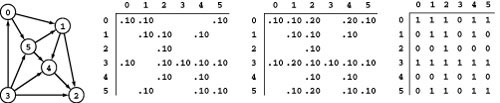
Given a digraph (left), we can transform its adjacency matrix (with self-loops) into an adjacency matrix representing a network by assigning an arbitrary weight to each edge (left matrix). As usual, blank entries in the matrix represent a sentinel value that indicates the absence of an edge. Given the all-pairs shortest-paths-lengths matrix of that network (center matrix), the transitive closure of the digraph (right matrix) is simply the matrix formed by subsituting 0 for each sentinel and 1 for all other entries.

Proof: We have already pointed out the direct relationship between Warshall’s algorithm and Floyd’s algorithm. Another way to consider that relationship, in the present context, is to imagine that we need to compute the transitive closure of digraphs using a library function that computes all shortest paths in networks. To do so, we add self-loops if they are not present in the digraph; then, we build a network directly from the adjacency matrix of the digraph, with an arbitrary weight (say 0.1) corresponding to each 1 and the sentinel weight corresponding to each 0. Then, we call the all-pairs shortest-paths function. Next, we can easily compute the transitive closure from the all-pairs shortest-paths matrix that the function computes: Given any two vertices u and v, there is a path from u to v in the digraph if and only if the length of the path from u to v in the network is nonzero (see Figure 21.21).

This property is a formal statement that the transitive-closure problem is no more difficult than the all-pairs shortest-paths problem. Since we happen to know algorithms for transitive closure that are even faster than the algorithms that we know for all-pairs shortest-paths problems, this information is no surprise. Reduction is more interesting when we use it to establish a relationship between problems that we do not know how to solve, or between such problems and other problems that we can solve.

Property 21.13 In networks with no constraints on edge weights, the longest-path and shortest-path problems (single-source or all-pairs) are equivalent.

Proof: Given a shortest-path problem, negate all the weights. A longest path (a path with the highest weight) in the modified network is a shortest path in the original network. An identical argument shows that the shortest-path problem reduces to the longest-path problem.

This proof is trivial, but this property also illustrates that care is justified in stating and proving reductions, because it is easy to take reductions for granted and thus to be misled. For example, it is decidedly not true that the longest-path and shortest-path problems are equivalent in networks with nonnegative weights.

At the beginning of this chapter, we outlined an argument that shows that the problem of finding shortest paths in undirected weighted graphs reduces to the problem of finding shortest paths in networks, so we can use our algorithms for networks to solve shortest-paths problems in undirected weighted graphs. Two further points about this reduction are worth contemplating in the present context. First, the converse does not hold: Knowing how to solve shortest-paths problems in undirected weighted graphs does not help us to solve them in networks. Second, we saw a flaw in the argument: If edge weights could be negative, the reduction gives networks with negative cycles, and we do not know how to find shortest paths in such networks. Even though the reduction fails, it turns out to be still possible to find shortest paths in undirected weighted graphs with no negative cycles with an unexpectedly complicated algorithm (see reference section). Since this problem does not reduce to the directed version, this algorithm does not help us to solve the shortest-path problem in general networks.

The concept of reduction essentially describes the process of using one ADT to implement another, as is done routinely by modern systems programmers. If two problems are equivalent, we know that if we can solve either of them efficiently, we can solve the other efficiently. We often find simple one-to-one correspondences, such as the one in Property 21.13, that show two problems to be equivalent. In this case, we have not yet discussed how to solve either problem, but it is useful to know that if we could find an efficient solution to one of them, we could use that solution to solve the other one. We saw another example in Chapter 17: When faced with the problem of determining whether or not a graph has an odd cycle, we noted that the problem is equivalent to determining whether or not the graph is two-colorable.

Reduction has two primary applications in the design and analysis of algorithms. First, it helps us to classify problems according to their difficulty at an appropriate abstract level without necessarily developing and analyzing full implementations. Second, we often do reductions to establish lower bounds on the difficulty of solving various problems, to help indicate when to stop looking for better algorithms. We have seen examples of these uses in Sections 19.3 and 20.7;we see others later in this section.

Beyond these direct practical uses, the concept of reduction also has widespread and profound implications for the theory of computation; these implications are important for us to understand as we tackle increasingly difficult problems. We discuss this topic briefly at the end of this section and consider it in full formal detail in Part 8.

The constraint that the cost of the transformations should not dominate is a natural one and often applies. In many cases, however, we might choose to use reduction even when the cost of the transformations does dominate. One of the most important uses of reduction is to provide efficient solutions to problems that might otherwise seem intractable by performing a transformation to a well-understood problem that we know how to solve efficiently. Reducing A to B, even if computing the transformations is much more expensive than is solving B, may give us a much more efficient algorithm for solving A than we could otherwise devise. There are many other possibilities. Perhaps we are interested in expected cost rather than the worst case. Perhaps we need to solve two problems B and C to solve A. Perhaps we need to solve multiple instances of B. We leave further discussion of such variations until Part 8, because all the examples that we consider before then are of the simple type just discussed.

In the particular case where we solve a problem A by simplifying another problem B, we know that A reduces to B, but not necessarily vice versa. For example, selection reduces to sorting because we can find the kth smallest element in a file by sorting the file and then indexing (or scanning) to the kth position, but this fact certainly does not imply that sorting reduces to selection. In the present context, the shortest-paths problem for weighted DAGs and the shortest-paths problem for networks with positive weights both reduce to the general shortest-paths problem. This use of reduction corresponds to the intuitive notion of one problem being more general than another. Any sorting algorithm solves any selection problem, and, if we can solve the shortest-paths problem in general networks, we certainly can use that solution for networks with various restrictions; but the converse is not necessarily true.

Figure 21.22 Job scheduling

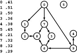
In this network, vertices represent jobs to be completed (with weights indicating the amount of time required) and edges represent precedence relationships between them. For example, the edges from 7 to 8 and 3 mean that job 7 must be finished before job 8 or job 3 can be started. What is the minimum amount of time required to complete all the jobs?

This use of reduction is helpful, but the concept becomes more useful when we use it to gain information about the relationships between problems in different domains. For example, consider the following problems, which seem at first blush to be far removed from graph processing. Through reduction, we can develop specific relationships between these problems and the shortest-paths problem.

Job scheduling A large set of jobs, of varying durations, needs to be performed. We can be working on any number of jobs at a given time, but a set of precedence relationships specify, for a set of pairs of jobs, that the first must be completed before the second can be started. What is the minimum amount of time required to complete all the jobs while satisfying all the precedence constraints? Specifically, given a set of jobs (with durations) and a set of precedence constraints, schedule the jobs (find a start time for each) so as to achieve this minimum.

Figure 21.22 depicts an example instance of the job-scheduling problem. It uses a natural network representation, which we use in a moment as the basis for a reduction. This version of the problem is perhaps the simplest of literally hundreds of versions that have been studied—versions that involve other job characteristics and other constraints, such as the assignment of personnel or other resources to the jobs, other costs associated with specific jobs, deadlines, and so forth. In this context, the version that we have described is commonly called precedence-constrained scheduling with unlimited parallelism; we use the term job scheduling as shorthand.

To help us to develop an algorithm that solves the job-scheduling problem, we consider the following problem, which is widely applicable in its own right.

Difference constraints Assign nonnegative values to a set variables x₀ through x_n that minimize the value of x_n while satisfying a set of difference constraints on the variables, each of which specifies that the difference between two of the variables must be greater than or equal to a given constant.

Figure 21.23 depicts an example instance of this problem. It is a purely abstract mathematical formulation that can serve as the basis for solving numerous practical problems (see reference section).

The difference-constraint problem is a special case of a much more general problem where we allow general linear combinations of the variables in the equations.

Figure 21.23 Difference constraints

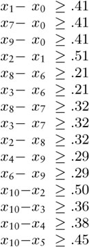
Finding an assignment of nonnegative values to the variables that minimizes the value of x₁₀ subject to this set of inequalities is equivalent to the job-scheduling problem instance illustrated in Figure 21.22. For example, the equation x₈x₇ +. 32 means that job 8 cannot start until job 7 is completed.

Linear programming Assign nonnegative values to a set of variables x ₀ through x _n that minimize the value of a specified linear combination of the variables, subject to a set of constraints on the variables, each of which specifies that a given linear combination of the variables must be greater than or equal to a given constant.

Linear programming is a widely used general approach to solving a broad class of optimization problems that we will not consider it in detail until Part 8. Clearly, the difference-constraints problem reduces to linear programming, as do many other problems. For the moment, our interest is in the relationships among the difference-constraints, job-scheduling, and shortest-paths problems.

Property 21.14 The job-scheduling problem reduces to the difference-constraints problem.

Proof: Add a dummy job and a precedence constraint for each job saying that the job must finish before the dummy job starts. Given a job-scheduling problem, define a system of difference equations where each job i corresponds to a variable x_i, and the constraint that j cannot start until i finishes corresponds to the equation x_j ≥ x_i + c_i, where c_i is the length of job i. The solution to the difference-constraints problem gives precisely a solution to the job-scheduling problem, with the value of each variable specifying the start time of the corresponding job.

Figure 21.23 illustrates the system of difference equations created by this reduction for the job-scheduling problem in Figure 21.22. The practical significance of this reduction is that we can use to solve job-scheduling problems any algorithm that can solve difference-constraint problems.

It is instructive to consider whether we can use this construction in the opposite way: Given a job-scheduling algorithm, can we use it to solve difference-constraints problems? The answer to this question is that the correspondence in the proof of Property 21.14 does not help us to show that the difference-constraints problem reduces to the job-scheduling problem, because the systems of difference equations that we get from job-scheduling problems have a property that does not necessarily hold in every difference-constraints problem. Specifically, if two equations have the same second variable, then they have the same constant. Therefore, an algorithm for job scheduling does not immediately give a direct way to solve a system of difference equations that contains two equations x_i −x_j ≥ a and x_k − x_j ≥ b, where a ≠ b. When proving reductions, we need to be aware of situations like this: A proof that A reduces to B must show that we can use an algorithm for solving B to solve any instance of A.

By construction, the constants in the difference-constraints problems produced by the construction in the proof of Property 21.14 are always nonnegative. This fact turns out to be significant.

Property 21.15 The difference-constraints problem with positive constants is equivalent to the single-source longest-paths problem in an acyclic network.

Proof: Given a system of difference equations, build a network where each variable x_i corresponds to a vertex i and each equation x_i x_j c corresponds to an edge i-j of weight c. For example, assigning to each edge in the digraph of Figure 21.22 the weight of its source vertex gives the network corresponding to the set of difference equations in Figure 21.23. Add a dummy vertex to the network, with a zero-weight edge to every other vertex. If the network has a cycle, the system of difference equations has no solution (because the positive weights imply that the values of the variables corresponding to each vertex strictly decrease as we move along a path, and, therefore, a cycle would imply that some variable is less than itself), so report that fact. Otherwise, the network has no cycle, so solve the single-source longest-paths problem from the dummy vertex. There exists a longest path for every vertex because the network is acyclic (see Section 21.4). Assign to each variable the length of the longest path to the corresponding vertex in the network from the dummy vertex. For each variable, this path is evidence that its value satisfies the constraints and that no smaller value does so.

Unlike the proof of Property 21.14, this proof does extend to show that the two problems are equivalent because the construction works in both directions. We have no constraint that two equations with the same second variable in the equation must have the same constants, and no constraint that edges leaving any given vertex in the network must have the same weight. Given any acyclic network with positive weights, the same correspondence gives a system of difference constraints with positive constants whose solution directly yields a

solution to the single-source longest-paths problem in the network. Details of this proof are left as an exercise (see Exercise 21.90).

The network in Figure 21.22 depicts this correspondence for our sample problem, and Figure 21.15 shows the computation of the longest paths in the network, using Program 21.6 (the dummy start vertex is implicit in the implementation). The schedule that is computed in this way is shown in Figure 21.24.

Figure 21.24 Job schedule

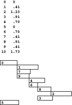
This figure illustrates the solution to the job-scheduling problem of Figure 21.22, derived from the correspondence between longest paths in weighted DAGs and job schedules. The longest path lengths in the wt array that is computed by the longest paths algorithm in Program 21.6 (see Figure 21.15) are precisely the required job start times (top, right column). We start jobs 0 and 5 at time 0, jobs 1, 7, and 9 at time .41, jobs 4 and 6 at time .70, and so forth.

Program 21.8 is an implementation that shows the application of this theory in a practical setting. It transforms any instance of the job-scheduling problem into an instance of the longest-path problem in acyclic networks, then uses Program 21.6 to solve it.

We have been implicitly assuming that a solution exists for any instance of the job-scheduling problem; however, if there is a cycle in the set of precedence constraints, then there is no way to schedule the jobs to meet them. Before looking for longest paths, we should check for this condition by checking whether the corresponding network has a cycle (see Exercise 21.100). Such a situation is typical, and a specific technical term is normally used to describe it.

Definition 21.4 A problem instance that admits no solution is said to be infeasible.

In other words, for job-scheduling problems, the question of determining whether a job-scheduling problem instance is feasible reduces to the problem of determining whether a digraph is acyclic. As we move to ever-more-complicated problems, the question of feasibility becomes an ever-more-important (and ever-more-difficult!) part of our computational burden.

We have now considered three interrelated problems. We might have shown directly that the job-scheduling problem reduces to the single-source longest-paths problem in acyclic networks, but we have also shown that we can solve any difference-constraints problem (with positive constants) in a similar manner (see Exercise 21.94), as well as any other problem that reduces to a difference-constraints problem or a job-scheduling problem. We could, alternatively, develop an algorithm to solve the difference-constraints problem and use that algorithm to solve the other problems, but we have not shown that a solution to the job-scheduling problem would give us a way to solve the others.

These examples illustrate the use of reduction to broaden the applicability of proven implementations. Indeed, modern systems programming emphasizes the need to reuse software by developing new interfaces and using existing software resources to build implementations. This important process, which is sometimes referred to as library programming, is a practical realization of the idea of reduction.

Library programming is extremely important in practice, but it represents only part of the story of the implications of reduction. To illustrate this point, we consider the following version of the job-scheduling problem.

Job scheduling with deadlines Allow an additional type of constraint in the job-scheduling problem, to specify that a job must begin before a specified amount of time has elapsed, relative to another job. (Conventional deadlines are relative to the start job.) Such constraints are commonly needed in time-critical manufacturing processes and in many other applications, and they can make the job-scheduling problem considerably more difficult to solve.

Suppose that we need to add a constraint to our example of Figures 21.22 through 21.24 that job 2 must start earlier than a certain number c of time units after job 4 starts. If c is greater than .53, then the schedule that we have computed fits the bill, since it says to start job 2 at time 1.23, which is .53 after the end time of job 4 (which starts at .70). If c is less than .53, we can shift the start time of 4 later to meet the constraint. If job 4 were a long job, this change could increase the finish time of the whole schedule. Worse, if there are other constraints on job 4, we may not be able to shift its start time. Indeed, we may find ourselves with constraints that no schedule can meet: For instance, we could not satisfy a constraint in our example that job 2 must start earlier than d time units after the start of job 6 for d less than .53 because the constraints that 2 must follow 8 and 8 must follow 6 imply that 2 must start later than .53 time units after the start of 6.

If we add both of the two constraints described in the previous paragraph to the example, then both of them affect the time that 4 can be scheduled, the finish time of the whole schedule, and whether a feasible schedule exists, depending on the values of c and d. Adding more constraints of this type multiplies the possibilities and turns an easy problem into a difficult one. Therefore, we are justified in seeking the approach of reducing the problem to a known problem.

Property 21.16 The job-scheduling-with-deadlines problem reduces to the shortest-paths problem (with negative weights allowed).

Proof: Convert precedence constraints to inequalities using the same reduction described in Property 21.14. For any deadline constraint, add an inequality x_i−x _j ≤ d_j, or, equivalently x_j−x_i≥−d_j, where d_j is a positive constant. Convert the set of inequalities to a network using the same reduction described in Property 21.15. Negate all the weights. By the same construction given in the proof of Property 21.15, any shortest-path tree rooted at 0 in the network corresponds to a schedule.

This reduction takes us to the realm of shortest paths with negative weights. It says that if we can find an efficient solution to the shortest-paths problem with negative weights, then we can find an efficient solution to the job-scheduling problem with deadlines. (Again, the correspondence in the proof of Property 21.16 does not establish the converse (see Exercise 21.91).)

Adding deadlines to the job-scheduling problem corresponds to allowing negative constants in the difference-constraints problem and negative weights in the shortest-paths problem. (This change also requires that we modify the difference-constraints problem to properly handle the analog of negative cycles in the shortest paths problem.) These more general versions of these problems are more difficult to solve than the versions that we first considered, but they are also likely to be more useful as more general models. A plausible approach to solving all of them would seem to be to seek an efficient solution to the shortest-paths problem with negative weights.

Unfortunately, there is a fundamental difficulty with this approach, and it illustrates the other part of the story in the use of reduction to assess the relative difficulty of problems. We have been using reduction in a positive sense, to expand the applicability of solutions to general problems; but it also applies in a negative sense, to show the limits on such expansion.

The difficulty is that the general shortest-paths problem is too hard to solve. We see next how the concept of reduction helps us to make this statement with precision and conviction. In Section 17.8, we discussed a set of problems, known as the NP-hard problems, that we consider to be intractable because all known algorithms for solving them require exponential time in the worst case. We show here that the general shortest-paths problem is NP-hard.

As mentioned briefly in Section 17.8 and discussed in detail in Part 8, we generally take the fact that a problem is NP-hard to mean not just that no efficient algorithm is known that is guaranteed to solve the problem but also that we have little hope of finding one. In this context, we use the term efficient to refer to algorithms whose running time is bounded by some polynomial function of the size of the input, in the worst case. We assume that the discovery of an efficient algorithm to solve any NP-hard problem would be a stunning research breakthrough. The concept of NP-hardness is important in identifying problems that are difficult to solve, because it is often easy to prove that a problem is NP-hard, using the following technique.

Property 21.17 A problem is NP-hard if there is an efficient reduction to it from any NP-hard problem.

This property depends on the precise meaning of an efficient reduction from one problem A to another problem B. We defer such definitions to Part 8 (two different definitions are commonly used). For the moment, we simply use the term to cover the case where we have efficient algorithms both to transform an instance of A to an instance of B and to transform a solution of B to a solution of A.

Now, suppose that we have an efficient reduction from an NP-hard problem A to a given problem B. The proof is by contradiction: If we have an efficient algorithm for B, then we could use it to solve any instance of A in polynomial time, by reduction (transform the given instance of A to an instance of B, solve that problem, then transform the solution). But no known algorithm can make such a guarantee for A (because A is NP-hard), so the assumption that there exists a polynomial-time algorithm for B is incorrect: B is also NP-hard.

This technique is extremely important because people have used it to show a huge number of problems to be NP-hard, giving us a broad variety of problems from which to choose when we want to develop a proof that a new problem is NP-hard. For example, we encountered one of the classic NP-hard problems in Section 17.7. The Hamilton-path problem, which asks whether there is a simple path containing all the vertices in a given graph, was one of the first problems shown to be NP-hard (see reference section). It is easy to formulate as a shortest-paths problem, so Property 21.17 implies that the shortest-paths problem itself is NP-hard:

Property 21.18 In networks with edge weights that could be negative, shortest-paths problems are NP-hard.

Proof: Our proof consists of reducing the Hamilton-path problem to the shortest-paths problem. That is, we show that we could use any algorithm that can find shortest paths in networks with negative edge weights to solve the Hamilton-path problem. Given an undirected graph, we build a network with edges in both directions corresponding to each edge in the graph and with all edges having weight −1. The shortest (simple) path starting at any vertex in this network is of length 1 − V if and only if the graph has a Hamilton path. Note that this network is replete with negative cycles. Not only does every cycle in the graph correspond to a negative cycle in the network, but also every edge in the graph corresponds to a cycle of weight −2 in the network.

The implication of this construction is that the shortest-paths problem is NP-hard, because if we could develop an efficient algorithm for the shortest-paths problem in networks, then we would have an efficient algorithm for the Hamilton-path problem in graphs.

One response to the discovery that a given problem is NP-hard is to seek versions of that problem that we can solve. For shortest-paths problems, we are caught between having a host of efficient algorithms for acyclic networks or for networks in which edge weights are nonnegative and having no good solution for networks that could have cycles and negative weights. Are there other kinds of networks that we can address? That is the subject of Section 21.7. There, for example, we see that the job-scheduling-with-deadlines problem reduces to a version of the shortest-paths problem that we can solve efficiently. This situation is typical: As we address ever-more-difficult computational problems, we find ourselves working to identify the versions of those problems that we can expect to solve.

As these examples illustrate, reduction is a simple technique that is helpful in algorithm design, and we use it frequently. Either we can solve a new problem by proving that it reduces to a problem that we know how to solve, or we can prove that the new problem will be difficult by proving that a problem that we know to be difficult reduces to the problem in question.

Table 21.3 gives us a more detailed look at the various implications of reduction results among the four general problem classes that we discussed in Chapter 17. Note that there are several cases where a reduction provides no new information; for example, although selection reduces to sorting and the problem of finding longest paths in acyclic networks reduces to the problem of finding shortest paths in general networks, these facts shed no new light on the relative difficulty of the problems. In other cases, the reduction may or may not provide new information; in still other cases, the implications of a reduction are truly profound. To develop these concepts, we need a precise and formal description of reduction, as we discuss in detail in Part 8; here, we summarize informally the most important uses of reduction in practice, with examples that we have already seen.

Table 21.3 Reduction implications

This table summarizes some implications of reducing a problem A to another problem B, with examples that we have discussed in this section. The profound implications of cases 9 and 10 are so far-reaching that we generally assume that it is not possible to prove such reductions (see Part 8). Reduction is most useful in cases 1, 6, 11, and 16, to learn a new algorithm for A or prove a lower bound on B; in cases 13-15, to learn new algorithms for A; and in case 12, to learn the difficulty of B.

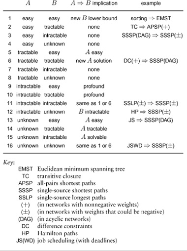
Upper bounds If we have an efficient algorithm for a problem B and can prove that A reduces to B, then we have an efficient algorithm for A. There may exist some other better algorithm for A, but B’s performance is an upper bound on the best that we can do for A. For example, our proof that job scheduling reduces to longest paths in acyclic networks makes our algorithm for the latter an efficient algorithm for the former.

Lower bounds If we know that any algorithm for problem A has certain resource requirements and we can prove that A reduces to B, then we know that B has at least those same resource requirements, because a better algorithm for B would imply the existence of a better algorithm for A (as long as the cost of the reduction is lower than the cost of B). That is, A’s performance is a lower bound on the best that we can do for B. For example, we used this technique in Section 19.3 to show that computing the transitive closure is as difficult as Boolean matrix multiplication, and we used it in Section 20.7 to show that computing the Euclidean MST is as difficult as sorting.

Intractability In particular, we can prove a problem to be intractable by showing that an intractable problem reduces to it. For example, Property 21.18 shows that the shortest-paths problem is intractable because the Hamilton-path problem reduces to the shortest-paths problem.

Beyond these general implications, it is clear that more detailed information about the performance of specific algorithms to solve specific problems can be directly relevant to other problems that reduce to the first ones. When we find an upper bound, we can analyze the associated algorithm, run empirical studies, and so forth to determine whether it represents a better solution to the problem. When we develop a good general-purpose algorithm, we can invest in developing and testing a good implementation and then develop associated ADTs that expand its applicability.

We use reduction as a basic tool in this and the next chapter. We emphasize the general relevance of the problems that we consider, and the general applicability of the algorithms that solve them, by reducing other problems to them. It is also important to be aware of a hierarchy among increasingly general problem-formulation models. For example, linear programming is a general formulation that is important not just because many problems reduce to it but also because it is not known to be NP-hard. In other words, there is no known way to reduce the general shortest-paths problem (or any other NP-hard problem) to linear programming. We discuss such issues in Part 8.

Not all problems can be solved, but good general models have been devised that are suitable for broad classes of problems that we do know how to solve. Shortest paths in networks is our first example of such a model. As we move to ever-more-general problem domains, we enter the field of operations research (OR), the study of mathematical methods of decision making, where developing and studying such models is central. One key challenge in OR is to find the model that is most appropriate for solving a problem and to fit the problem to the model. This activity is sometimes known as mathematical programming (a name given to it before the advent of computers and the new use of the word “programming”). Reduction is a modern concept that is in the same spirit as mathematical programming and is the basis for our understanding of the cost of computation in a broad variety of applications.

Exercises

• 21.85 Use the reduction of Property 21.12 to develop a transitive-closure implementation (with the same interface as Programs 19.3 and 19.4) that uses the all-pairs shortest-paths ADT of Section 21.3.

21.86 Show that the problem of computing the number of strong components in a digraph reduces to the all-pairs shortest-paths problem with nonnegative weights.

21.87 Give the difference-constraints and shortest-paths problems that correspond—according to the constructions of Properties 21.14 and 21.15—to the job-scheduling problem, where jobs 0 to 7 have lengths

.4 .2 .3 .4 .2 .5 .1

and constraints

5-1 4-6 6-0 3-2 6-1 6-2,

respectively.

• 21.88 Give a solution to the job-scheduling problem of Exercise 21.87.

• 21.89 Suppose that the jobs in Exercise 21.87 also have the constraints that job 1 must start before job 6 ends, and job 2 must start before job 4 ends. Give the shortest-paths problem to which this problem reduces, using the construction described in the proof of Property 21.16.

21.90 Show that the all-pairs longest-paths problem in acyclic networks with positive weights reduces to the difference-constraints problem with positive constants.

• 21.91 Explain why the correspondence in the proof of Property 21.16 does not extend to show that the shortest-paths problem reduces to the job-scheduling-with-deadlines problem.

21.92 Extend Program 21.8 to use symbolic names instead of integers to refer to jobs (see Program 17.10).

21.93 Design an ADT interface that provides clients with the ability to pose and solve difference-constraints problems.

21.94 Write a class that implements your interface from Exercise 21.93, basing your solution to the difference-constraints problem on a reduction to the shortest-paths problem in acyclic networks.

21.95 Provide an implementation for a class that solves the single-source shortest-paths problem in acyclic networks with negative weights, which is based on a reduction to the difference-constraints problem and uses your interface from Exercise 21.93.

• 21.96 Your solution to the shortest-paths problem in acyclic networks for Exercise 21.95 assumes the existence of an implementation that solves the difference-constraints problem. What happens if you use the implementation from Exercise 21.94, which assumes the existence of an implementation for the shortest-paths problem in acyclic networks?

• 21.97 Prove the equivalence of any two NP-hard problems (that is, choose two problems and prove that they reduce to each other).

•• 21.98 Give an explicit construction that reduces the shortest-paths problem in networks with integer weights to the Hamilton-path problem.

• 21.99 Use reduction to implement a class that uses a network ADT that solves the single-source shortest-paths problem to solve the following problem: Given a digraph, a vertex-indexed vector of positive weights, and a start vertex v, find the paths from v to each other vertex such that the sum of the weights of the vertices on the path is minimized.

• 21.100 Program 21.8 does not check whether the job-scheduling problem that it takes as input is feasible (has a cycle). Characterize the schedules that it prints out for infeasible problems.

21.101 Design an ADT interface that gives clients the ability to pose and solve job-scheduling problems. Write a class that implements your interface, basing your solution to the job-scheduling problem on a reduction to the shortest-paths problem in acyclic networks, as in Program 21.8.

• 21.102 Add a function to your class from Exercise 21.101 (and provide an implementation) that prints out a longest path in the schedule. (Such a path is known as a critical path.)

21.103 Write a client for your interface from Exercise 21.101 that outputs a PostScript program that draws the schedule in the style of Figure 21.24 (see Section 4.3).

• 21.104 Develop a model for generating job-scheduling problems. Use this model to test your implementations of Exercises 21.101 and 21.103 for a reasonable set of problem sizes.

21.105 Write a class that implements your interface from Exercise 21.101, basing your solution to the job-scheduling problem on a reduction to the difference-constraints problem.

• 21.106 A PERT (performance-evaluation-review-technique) chart is a network that represents a job-scheduling problem, with edges representing jobs, as described in Figure 21.25. Write a class that implements your job-scheduling interface of Exercise 21.101 that is based on PERT charts.

21.107 How many vertices are there in a PERT chart for a job-scheduling problem with V jobs and E constraints?

21.108 Write programs to convert between the edge-based job-scheduling representation (PERT chart) discussed in Exercise 21.106 and the vertex-based representation used in the text (see Figure 21.22).

Figure 21.25 A PERT chart

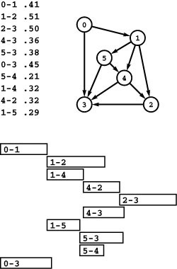
A PERT chart is a network representation for job-scheduling problems where we represent jobs by edges. The network at the top is a representation of the job-scheduling problem depicted in Figure 21.22, where jobs 0 through 9 in Figure 21.22 are represented by edges 0-1, 1-2, 2-3, 4-3, 5-3, 0-3, 5-4, 1-4, 4-2, and 1-5, respectively, here. The critical path in the schedule is the longest path in the network.

21.7 Negative Weights

We now turn to the challenge of coping with negative weights in shortest-paths problems. Perhaps negative edge weights seem unlikely, given our focus through most of this chapter on intuitive examples, where weights represent distances or costs; however, we also saw in Section 21.6 that negative edge weights arise in a natural way when we reduce other problems to shortest-paths problems. Negative weights are not merely a mathematical curiosity; on the contrary, they significantly extend the applicability of the shortest-paths problems as a model for solving other problems. This potential utility is our motivation to search for efficient algorithms to solve network problems that involve negative weights.

Figure 21.26 is a small example that illustrates the effects of introducing negative weights on a network’s shortest paths. Perhaps the most important effect is that when negative weights are present, low-weight shortest paths tend to have more edges than higher-weight paths. For positive weights, our emphasis was on looking for shortcuts; but when negative weights are present, we seek detours that use as many edges with negative weights as we can find. This effect turns our intuition in seeking “short” paths into a liability in understanding the algorithms, so we need to suppress that line of intuition and consider the problem on a basic abstract level.

Figure 21.26 A sample network with negative edges

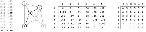
This sample network is the same as the network depicted in Figure 21.1, except that the edges 3-5 and 5-1 are negative. Naturally, this change dramatically affects the shortest paths structure, as we can easily see by comparing the distance and path matrices at the right with their counterparts in Figure 21.9. For example, the shortest path from 0 to 1 in this network is 0-5-1, which is of length 0; and the shortest path from 2 to 1 is 2-3-5-1, which is of length -.17.

The relationship shown in the proof of Property 21.18 between shortest paths in networks and Hamilton paths in graphs ties in with our observation that finding paths of low weight (which we have been calling “short”) is tantamount to finding paths with a high number of edges (which we might consider to be “long”). With negative weights, we are looking for long paths rather than short paths.

The first idea that suggests itself to remedy the situation is to find the smallest (most negative) edge weight, then to add the absolute value of that number to all the edge weights to transform the network into one with no negative weights. This naive approach does not work at all, because shortest paths in the new network bear little relation to shortest paths in the old one. For example, in the network illustrated in Figure 21.26, the shortest path from 4 to 2 is 4-3-5-1-2. If we add .38 to all the edge weights in the graph to make them all positive, the weight of this path grows from .20 to 1.74. But the weight of 4-2 grows from .32 to just .70, so that edge becomes the shortest path from 4 to 2. The more edges a path has, the more it is penalized by this transformation; that result, from the observation in the previous paragraph, is precisely the opposite of what we need. Even though this naive idea does not work, the goal of transforming the network into an equivalent one with no negative weights but the same shortest paths is worthy; at the end of the section, we consider an algorithm that achieves this goal.

Our shortest-paths algorithms to this point have all placed one of two restrictions on the shortest-paths problem so that they can offer an efficient solution: They either disallow cycles or disallow negative weights. Is there a less stringent restriction that we could impose on networks that contain both cycles and negative weights that would still lead to tractable shortest-paths problems? We touched on an answer to this question at the beginning of the chapter, when we had to add the restriction that paths be simple so that the problem would make sense if there were negative cycles. Should we perhaps restrict attention to networks that have no such cycles?

Shortest paths in networks with no negative cycles Given a network that may have negative edge weights but does not have any negative-weight cycles, solve one of the following problems: Find a shortest path connecting two given vertices (shortest-path problem), find shortest paths from a given vertex to all the other vertices (single-source problem), or find shortest paths connecting all pairs of vertices (all-pairs problem).

The proof of Property 21.18 leaves the door open for the possibility of efficient algorithms for solving this problem because it breaks down if we disallow negative cycles. To solve the Hamilton-path problem, we would need to be able to solve shortest-paths problems in networks that have huge numbers of negative cycles.

Moreover, many practical problems reduce precisely to the problem of finding shortest paths in networks that contain no negative cycles. We have already seen one such example.

Property 21.19 The job-scheduling-with-deadlines problem reduces to the shortest-paths problem in networks that contain no negative cycles.

Proof: The argument that we used in the proof of Property 21.15 shows that the construction in the proof of Property 21.16 leads to networks that contain no negative cycles. From the job-scheduling problem, we construct a difference-constraints problem with variables that correspond to job start times; from the difference-constraints problem, we construct a network. We negate all the weights to convert from a longest-paths problem to a shortest-paths problem—a transformation that corresponds to reversing the sense of all the inequalities. Any simple path from i to j in the network corresponds to a sequence of inequalities involving the variables. The existence of the path implies, by collapsing these inequalities, that x_i − x_j ≤ w_ij, where w_ij is the sum of the weights on the path from i to j. A negative cycle corresponds to 0 on the left side of this inequality and a negative value on the right, so the existence of such a cycle is a contradiction. •

Figure 21.27 Arbitrage

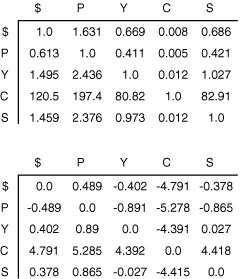
The table at the top specifies conversion factors from one currency to another. For example, the second entry in the top row says that $1 buys 1.631 units of currency P. Converting $1000 to currency P and back again would yield $1000*(1.631)*(0.613) = $999, a loss of $1. But converting $1000 to currency P then to currency Y and back again yields $1000*(1.631)*(0.411)*(1.495) = $1002, a .2% arbitrage opportunity. If we take the negative of the logarithm of all the numbers in the table (bottom), we can consider it to be the adjacency matrix for a complete network with edge weights that could be positive or negative. In this network, nodes correspond to currencies, edges to conversions, and paths to sequences of conversions. The conversion just described corresponds to the cycle $-P-Y-$ in the graph, which has weight −0.489 + 0.890 − 0.402 =. 002. The best arbitrage opportunity is the shortest cycle in the graph.

As we noted when we first discussed the job-scheduling problem in Section 21.6, this statement implicitly assumes that our job-scheduling problems are feasible (have a solution). In practice, we would not make such an assumption, and part of our computational burden would be determining whether or not a job-scheduling-with-deadlines problem is feasible. In the construction in the proof of Property 21.19, a negative cycle in the network implies an infeasible problem, so this task corresponds to the following problem.

Negative cycle detection Does a given network have a negative cycle? If it does, find one such cycle.

On the one hand, this problem is not necessarily easy (a simple cycle-checking algorithm for digraphs does not apply); on the other hand, it is not necessarily difficult (the reduction of Property 21.16 from the Hamilton-path problem does not apply). Our first challenge will be to develop an algorithm for this task.

In the job-scheduling-with-deadlines application, negative cycles correspond to error conditions that are presumably rare, but for which we need to check. We might even develop algorithms that remove edges to break the negative cycle and iterate until there are none. In other applications, detecting negative cycles is the prime objective, as in the following example.

Arbitrage Many newspapers print tables showing conversion rates among the world’s currencies (see, for example, Figure 21.27). We can view such tables as adjacency-matrix representations of complete networks. An edge s-t with weight x means that we can convert 1 unit of currency s into x units of currency t. Paths in the network specify multistep conversions. For example, if there is also an edge t-w with weight y, then the path s-t-w represents a way to convert 1 unit of currency s into xy units of currency w. We might expect xy to be equal to the weight of s-w in all cases, but such tables represent a complex dynamic system where such consistency cannot be guaranteed. If we find a case where xy is smaller than the weight of s-w, then we may be able to outsmart the system. Suppose that the weight of w-s is z and xyz > 1, then the cycle s-t-w-s gives a way to convert 1 unit of currency s into more than 1 units (xyz) of currency s. That is, we can make a 100(xyz − 1) percent profit by converting from s to t to w back to s. This situation is an example of an arbitrage opportunity that would allow us to make unlimited profits were it not for forces outside the model, such as limitations on the size of transactions. To convert this problem to a shortest-paths problem, we take the logarithm of all the numbers so that path weights correspond to adding edge weights instead of multiplying them, and then we take the negative to invert the comparison. Then the edge weights might be negative or positive, and a shortest path from s to t gives a best way of converting from currency s to currency t. The lowest-weight cycle is the best arbitrage opportunity, but any negative cycle is of interest.

Figure 21.28 Failure of Dijkstra’s algorithm (negative weights)

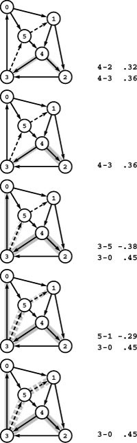
In this example, Dijkstra’s algorithm decides that 4-2 is the shortest path from 4 to 2 (of length .32) and misses the shorter path 4-3-5-1-2 (of length .20).

Can we detect negative cycles in a network or find shortest paths in networks that contain no negative cycles? The existence of efficient algorithms to solve these problems does not contradict the NP-hardness of the general problem that we proved in Property 21.18, because no reduction from the Hamilton-path problem to either problem is known. Specifically, the reduction of Property 21.18 says that what we cannot do is to craft an algorithm that can guarantee to find efficiently the lowest-weight path in any given network when negative edge weights are allowed. That problem statement is too general. But we can solve the restricted versions of the problem just mentioned, albeit not as easily as we can the other restricted versions of the problem (positive weights and acyclic networks) that we studied earlier in this chapter.

In general, as we noted in Section 21.2, Dijkstra’s algorithm does not work in the presence of negative weights, even when we restrict attention to networks that contain no negative cycles. Figure 21.28 illustrates this fact. The fundamental difficulty is that the algorithm depends on examining paths in increasing order of their length. The proof that the algorithm is correct (see Property 21.2) assumes that adding an edge to a path makes that path longer.

Floyd’s algorithm makes no such assumption and is effective even when edge weights may be negative. If there are no negative cycles, it computes shortest paths; remarkably enough, if there are negative cycles, it detects at least one of them.

Property 21.20 Floyd’s algorithm solves the negative-cycle–detection problem and the all-pairs shortest-paths problem in networks that contain no negative cycles, in time proportional to V³.

Proof: The proof of Property 21.8 does not depend on whether or not edge weights are negative; however, we need to interpret the results differently when negative edge weights are present. Each entry in the matrix is evidence of the algorithm having discovered a path of that length; in particular, any negative entry on the diagonal of the distances matrix is evidence of the presence of at least one negative cycle. In the presence of negative cycles, we cannot directly infer any further information, because the paths that the algorithm implicitly tests are not necessarily simple: Some may involve one or more trips around one or more negative cycles. However, if there are no negative cycles, then the paths that are computed by the algorithm are simple, because any path with a cycle would imply the existence of a path that connects the same two points which has fewer edges and is not of higher weight (the same path with the cycle removed).

The proof of Property 21.20 does not give specific information about how to find a specific negative cycle from the distances and paths matrices computed by Floyd’s algorithm. We leave that task for an exercise (see Exercise 21.122).

Floyd’s algorithm solves the all-pairs shortest-paths problem for graphs that contain no negative cycles. Given the failure of Dijkstra’s algorithm in networks that contain weights that could be negative, we could also use Floyd’s algorithm to solve the the all-pairs problem for sparse networks that contain no negative cycles, in time proportional to V³. If we have a single-source problem in such networks, then we can use this V³ solution to the all-pairs problem that, although it amounts to overkill, is the best that we have yet seen for the single-source problem. Can we develop faster algorithms for these problems—ones that achieve the running times that we achieve with Dijkstra’s algorithm when edge weights are positive (E lg V for single-source shortest paths and V E lg V for all-pairs shortest paths)? We can answer this question in the affirmative for the all-pairs problem and also can bring down the worst-case cost to V E for the single-source problem, but breaking the V E barrier for the general single-source shortest-paths problem is a longstanding open problem.

The following approach, developed by R. Bellman and L. Ford in the late 1950s, provides a simple and effective basis for attacking single-source shortest-paths problems in networks that contain no negative cycles. To compute shortest paths from a vertex s, we maintain (as usual) a vertex-indexed vector wt such that wt[t] contains the shortest-path length from s to t. We initialize wt[s] to 0 and all other

Figure 21.29 Floyd’s algorithm (negative weights)

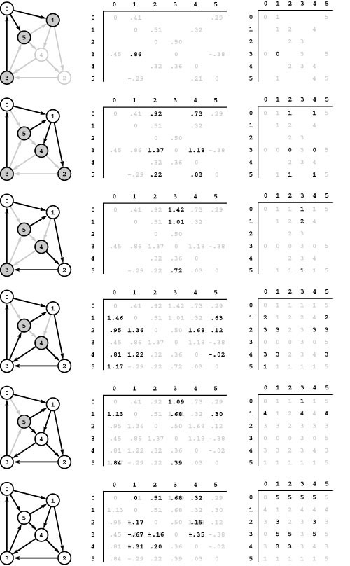
This sequence shows the construction of the all–shortest-paths matrices for a digraph with negative weights, using Floyd’s algorithm. The first step is the same as depicted in Figure 21.14. Then the negative edge 5-1 comes into play in the second step, where the paths 5-1-2 and 5-1-4 are discovered. The algorithm involves precisely the same sequence of relaxation steps for any edge weights, but the outcome differs.

wt entries to a large sentinel value, then compute shortest paths as follows:

We use the term Bellman–Ford algorithm to refer to the generic method of making V passes through the edges, considering the edges in any order. Certain authors use the term to describe a more general method (see Exercise 21.130).

For example, in a graph represented with adjacency lists, we could implement the Bellman–Ford algorithm to find the shortest paths from a start vertex s by initializing the wt entries to a value larger than any path length and the spt entries to null pointers, then proceeding as follows:

wt[s] = 0;
for (i = 0; i < G->V(); i++)
  for (v = 0; v < G->V(); v++)
  {
    if (v != s && spt[v] == 0) continue;
    typename Graph::adjIterator A(G, v);
    for (Edge* e = A.beg(); !A.end(); e = A.nxt())
     if (wt[e->w()] > wt[v] + e->wt())
     { wt[e->w()] = wt[v] + e->wt(); st[e->w()] = e; }
  }

This code exhibits the simplicity of the basic method. It is not used in practice, however, because simple modifications yield implementations that are more efficient for most graphs, as we soon see.

Property 21.21 With the Bellman–Ford algorithm, we can solve the single-source shortest-paths problem in networks that contain no negative cycles in time proportional to V E.

Proof:We make V passes through all E edges, so the total time is proportional to V E. To show that the computation achieves the desired result, we show by induction on i that, after the ith pass, wt[v] is no greater than the length of the shortest path from s to v that contains i or fewer edges, for all vertices v. The claim is certainly true if i is 0. Assuming the claim to be true for i, there are two cases for each given vertex v: Among the paths from s to v with i+1 or fewer edges, there may or may not be a shortest path with i+1 edges. If the shortest of the paths with i+1 or fewer edges from s to v is of length i or less,

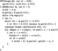
then wt[v] will not change and will remain valid. Otherwise, there is a path from s to v with i+1 edges that is shorter than any path from s to v with i or fewer edges. That path must consist of a path with i edges from s to some vertex w plus the edge w-v. By the induction hypothesis, wt[w] is an upper bound on the shortest distance from s to w, and the (i+1)st pass checks whether each edge constitutes the final edge in a new shortest path to that edge’s destination. In particular, it checks the edge w-v.

After V-1 iterations, then, wt[v] is a lower bound on the length of any shortest path with V-1 or fewer edges from s to v, for all vertices v. We can stop after V-1 iterations because any path with V or more edges must have a (positive- or zero-cost) cycle and we could find a path with V-1 or fewer edges that is the same length or shorter by removing the cycle. Since wt[v] is the length of some path from s to v, it is also an upper bound on the shortest-path length, and therefore must be equal to the shortest-path length.

Although we did not consider it explicitly, the same proof shows that the spt vector contains pointers to the edges in the shortest-paths tree rooted at s.

For typical graphs, examining every edge on every pass is wasteful. Indeed, we can easily determine a priori that numerous edges are not going to lead to a successful relaxation in any given pass. In fact, the only edges that could lead to a change are those emanating from a vertex whose value changed on the previous pass.

Program 21.9 is a straightforward implementation where we use a FIFO queue to hold these edges so that they are the only ones examined on each pass. Figure 21.30 shows an example of this algorithm in operation.

Program 21.9 is effective for solving the single-source shortest-paths problem in networks that arise in practice, but its worst-case performance is still proportional to V E. For dense graphs, the running time is not better than for Floyd’s algorithm, which finds all shortest paths, rather than just those from a single source. For sparse graphs, the implementation of the Bellman–Ford algorithm in Program 21.9 is up to a factor of V faster than Floyd’s algorithm but is nearly a factor of V slower than the worst-case running time that we can achieve with Dijkstra’s algorithm for networks with no negative-weight edges (see Table 19.2).

Other variations of the Bellman–Ford algorithm have been studied, some of which are faster for the single-source problem than the FIFO-queue version in Program 21.9, but all take time proportional to at least V E in the worst case (see, for example, Exercise 21.132). The basic Bellman–Ford algorithm was developed decades ago; and, despite the dramatic strides in performance that we have seen for many other graph problems, we have not yet seen algorithms with better worst-case performance for networks with negative weights.

The Bellman–Ford algorithm is also a more efficient method than Floyd’s algorithm for detecting whether a network has negative cycles.

Figure 21.30 Bellman-Ford algorithm (with negative weights)

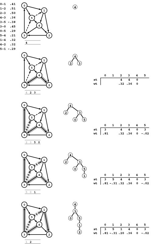
This figure shows the result of using the Bellman-Ford algorithm to find the shortest paths from vertex 4 in the network depicted in Figure Figure 21.26. The algorithm operates in passes, where we examine all edges emanating from all vertices on a FIFO queue. The contents of the queue are shown below each graph drawing, with the shaded entries representing the contents of the queue for the previous pass. When we find an edge that can reduce the length of a path from 4 to its destination, we do a relaxation operation that puts the destination vertex on the queue and the edge on the SPT. The gray edges in the graph drawings comprise the SPT after each stage, which is also shown in oriented form in the center (all edges pointing down). We begin with an empty SPT and 4 on the queue (top). In the second pass, we relax along 4-2 and 4-3, leaving 2 and 3 on the queue. In the third pass, we examine but do not relax along 2-3 and then relax along 3-0 and 3-5, leaving 0 and 5 on the queue. In the fourth pass, we relax along 5-1 and then examine but do not relax along 1-0 and 1-5, leaving 1 on the queue. In the last pass (bottom), we relax along 1-2. The algorithm initially operates like BFS, but, unlike all of our other graph search methods, it might change tree edges, as in the last step.

Property 21.22 With the Bellman–Ford algorithm, we can solve the negative-cycle–detection problem in time proportional to V E.

Proof: The basic induction in the proof of Property 21.21 is valid even in the presence of negative cycles. If we run a Vth iteration of the algorithm and any relaxation step succeeds, then we have found a shortest path with V edges that connects s to some vertex in the network. Any such path must have a cycle (connecting some vertex w to itself) and that cycle must be negative, by the inductive hypothesis, since the path from s to the second occurrence of w must be shorter than the path from s to the first occurrence of w for w to be included on the path the second time. The cycle will also be present in the tree; thus, we could also detect cycles by periodically checking the spt edges (see Exercise 21.134).

This argument holds for only those vertices that are in the same strongly connected component as the source s. To detect negative cycles in general, we can either compute the strongly connected components and initialize weights for one vertex in each component to 0 (see Exercise 21.126) or add a dummy vertex with edges to every other vertex (see Exercise 21.127).

To conclude this section, we consider the all-pairs shortest-paths problem. Can we do better than Floyd’s algorithm, which runs in time proportional to V³? Using the Bellman–Ford algorithm to solve the all-pairs problem by solving the single-source problem at each vertex exposes us to a worst-case running time that is proportional to V²E. We do not consider this solution in more detail because there is a way to guarantee that we can solve the all-paths problem in time proportional to V E log V. It is based on an idea that we considered at the beginning of this section: transforming the network into a network that has only nonnegative weights and that has the same shortest-paths structure.

In fact, we have a great deal of flexibility in transforming any network to another one with different edge weights but the same shortest paths. Suppose that a vertex-indexed vector wt contains an arbitrary assignment of weights to the vertices of a network G. With these weights, we define the operation of reweighting the graph as follows:

• To reweight an edge, add to that edge’s weight the difference between the weights of the edge’s source and destination.

• To reweight a network, reweight all of that network’s edges.

For example, the following straightforward code reweights a network, using our standard conventions:

for (v = 0; v < G->V(); v++)
  { typename Graph::adjIterator A(G, v);
    for (Edge* e = A.beg(); !A.end(); e = A.nxt())
      e->wt() = e->wt() + wt[v] - wt[e->w()]
  }

This operation is a simple linear-time process that is well-defined for all networks, regardless of the weights. Remarkably, the shortest paths in the transformed network are the same as the shortest paths in the original network.

Property 21.23 Reweighting a network does not affect its shortest paths.

Proof: Given any two vertices s and t, reweighting changes the weight of any path from s to t, precisely by adding the difference between the weights of s and t. This fact is easy to prove by induction on the length of the path. The weight of every path from s to t is changed by the same amount when we reweight the network, long paths and short paths alike. In particular, this fact implies immediately that the shortest-path length between any two vertices in the transformed network is the same as the shortest-path length between them in the original network.

Since paths between different pairs of vertices are reweighted differently, reweighting could affect questions that involve comparing shortest-path lengths (for example, computing the network’s diameter). In such cases, we need to invert the reweighting after completing the shortest-paths computation but before using the result.

Reweighting is no help in networks with negative cycles: The operation does not change the weight of any cycle, so we cannot remove negative cycles by reweighting. But for networks with no negative cycles, we can seek to discover a set of vertex weights such that reweighting leads to edge weights that are nonnegative, no matter what the original edge weights. With nonnegative edge weights, we can then solve the all-pairs shortest-paths problem with the all-pairs version of Dijkstra’s algorithm. For example, Figure 21.31 gives such an example for our sample network, and Figure 21.32 shows the shortest-paths computation with Dijkstra’s algorithm on the transformed network with no negative edges. The following property shows that we can always find such a set of weights.

Figure 21.31 Reweighting a network

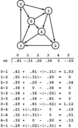
Given any assignment of weights to vertices (top), we can reweight all of the edges in a network by adding to each edge’s weight the difference of the weights of its source and destination vertices. Reweighting does not affect the shortest paths because it makes the same change to the weights of all paths connecting each pair of vertices. For example, consider the path 0-5-4-2-3: Its weight is .29 + .21 + .32 + .50 = 1.32; its weight in the reweighted network is 1.12 + .19 + .12 + .34 = 1.77; these weights differ by .45 = .81 - .36, the difference of the weights of 0 and 3; and the weights of all paths between 0 and 3 change by this same amount.

Property 21.24 In any network with no negative cycles, pick any vertex s and assign to each vertex v a weight equal to the length of a shortest path to v from s . Reweighting the network with these vertex weights yields nonnegative edge weights for each edge that connects vertices reachable from s.

Proof: Given any edge v-w, the weight of v is the length of a shortest path to v, and the weight of w is the length of a shortest path to w. If v-w is the final edge on a shortest path to w, then the difference between the weight of w and the weight of v is precisely the weight of v-w. In other words, reweighting the edge will give a weight of 0. If the shortest path through w does not go through v, then the weight of v plus the weight of v-w must be greater than or equal to the weight of w. In other words, reweighting the edge will give a positive weight.

Just as we did when we used the Bellman–Ford algorithm to detect negative cycles, we have two ways to proceed to make every edge weight nonnegative in an arbitrary network with no negative cycles. Either we can begin with a source from each strongly connected component, or we can add a dummy vertex with an edge of length 0 to every network vertex. In either case, the result is a shortest-paths spanning forest that we can use to assign weights to every vertex (weight of the path from the root to the vertex in its SPT).

For example, the weight values chosen in Figure 21.31 are precisely the lengths of shortest paths from 4, so the edges in the shortest-paths tree rooted at 4 have weight 0 in the reweighted network.

In summary, we can solve the all-pairs shortest-paths problem in networks that contain negative edge weights but no negative cycles by proceeding as follows:

• Apply the Bellman-Ford algorithm to find a shortest-paths forest in the original network.

• If the algorithm detects a negative cycle, report that fact and terminate.

• Reweight the network from the forest.

• Apply the all-pairs version of Dijkstra’s algorithm to the reweighted network.

Figure 21.32 All shortest paths in a reweighted network

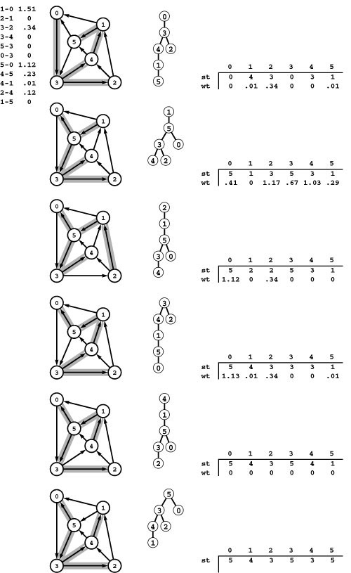
These diagrams depict the SPTs for each vertex in the reverse of the reweighted network from Figure 21.31, as could be computed with Dijkstra’s algorithm to give us shortest paths in the original network in Figure Figure 21.26. The paths are the same as for the network before reweighting, so, as in Figure 21.9, the st vectors in these diagrams are the columns of the paths matrix in Figure Figure 21.26. The wt vectors in this diagram correspond to the columns in the distances matrix, but we have to undo the reweighting for each entry by subtracting the weight of the source vertex and adding the weight of the final vertex in the path (see Figure 21.31). For example, from the third row from the bottom here we can see that the shortest path from 0 to 3 is 0-5-1-4-3 in both networks, and its length is 1.13 in the reweighted network shown here. Consulting Figure 21.31, we can calculate its length in the original network by subtracting the weight of 0 and adding the weight of 3 to get the result 1.13 - .81 + .36 = .68, the entry in row 0 and column 3 of the distances matrix in Figure Figure 21.26. All shortest paths to 4 in this network are of length 0 because we used those paths for reweighting.

After this computation, the paths matrix gives shortest paths in both networks, and the distances matrix give the path lengths in the reweighted network. This series of steps is sometimes known as John-son’s algorithm (see reference section).

Property 21.25 With Johnson’s algorithm, we can solve the all-pairs shortest-paths problem in networks that contain no negative cycles in time proportional to V E log_dV, where d =2if E < 2V, and d=E/V otherwise.

Proof: See Properties 21.22 through 21.24 and the summary in the previous paragraph. The worst-case bound on the running time is immediate from Properties 21.7 and 21.22.

To implement Johnson’s algorithm, we combine the implementation of Program 21.9, the reweighting code that we gave just before Property 21.23, and the all-pairs shortest-paths implementation of Dijkstra’s algorithm in Program 21.4 (or, for dense graphs, Program 20.6). As noted in the proof of Property 21.22, we have to make appropriate modifications to the Bellman–Ford algorithm for networks that are not strongly connected (see Exercises 21.135 through 21.137). To complete the implementation of the all-pairs shortest-paths interface, we can either compute the true path lengths by subtracting the weight of the start vertex and adding the weight of the destination vertex (undoing the reweighting operation for the paths) when copying the two vectors into the distances and paths matrices in Dijkstra’s algorithm, or we can put that computation in GRAPHdist in the ADT implementation.

For networks with no negative weights, the problem of detecting cycles is easier to solve than is the problem of computing shortest paths from a single source to all other vertices; the latter problem is easier to solve than is the problem of computing shortest paths connecting all pairs of vertices. These facts match our intuition. By contrast, the analogous facts for networks that contain negative weights are counterintuitive: The algorithms that we have discussed in this section show that, for networks that have negative weights, the best known algorithms for these three problems have similar worst-case performance characteristics. For example, it is nearly as difficult, in the worst case, to determine whether a network has a single negative cycle as it is to find all shortest paths in a network of the same size that has no negative cycles.

Exercises

• 21.109 Modify your random-network generators from Exercises 21.6 and 21.7 to generate weights between a and b (where a and b are both between −1 and 1), by rescaling.

• 21.110 Modify your random-network generators from Exercises 21.6 and 21.7 to generate negative weights by negating a fixed percentage (whose value is supplied by the client) of the edge weights.

• 21.111 Develop client programs that use your generators from Exercises 21.109 and 21.110 to produce networks that have a large percentage of negative weights but have at most a few negative cycles, for as large a range of values of V and E as possible.

21.112 Find a currency-conversion table online or in a newspaper. Use it to build an arbitrage table. Note: Avoid tables that are derived (calculated) from a few values and that therefore do not give sufficiently accurate conversion information to be interesting. Extra credit: Make a killing in the money-exchange market!

• 21.113 Build a sequence of arbitrage tables using the source for conversion that you found for Exercise 21.112 (any source publishes different tables periodically). Find all the arbitrage opportunities that you can in the tables, and try to find patterns among them. For example, do opportunities persist day after day, or are they fixed quickly after they arise?

21.114 Develop a model for generating random arbitrage problems. Your goal is to generate tables that are as similar as possible to the tables that you used in Exercise 21.113.

21.115 Develop a model for generating random job-scheduling problems that include deadlines. Your goal is to generate nontrivial problems that are likely to be feasible.

21.116 Modify your interface and implementations from Exercise 21.101 to give clients the ability to pose and solve job-scheduling problems that include deadlines, using a reduction to the shortest-paths problem.

• 21.117 Explain why the following argument is invalid: The shortest-paths problem reduces to the difference-constraints problem by the construction used in the proof of Property 21.15, and the difference-constraints problem reduces trivially to linear programming, so, by Property 21.17, linear programming is NP-hard.

21.118 Does the shortest-paths problem in networks with no negative cycles reduce to the job-scheduling problem with deadlines? (Are the two problems equivalent?) Prove your answer.

• 21.119 Find the lowest-weight cycle (best arbitrage opportunity) in the example shown in Figure 21.27.

• 21.120 Prove that finding the lowest-weight cycle in a network that may have negative edge weights is NP-hard.

• 21.121 Show that Dijkstra’s algorithm does work correctly for a network in which edges that leave the source are the only edges with negative weights.

• 21.122 Develop a class based on Floyd’s algorithm that provides clients with the capability to test networks for the existence of negative cycles.

21.123 Show, in the style of Figure 21.29, the computation of all shortest paths of the network defined in Exercise 21.1, with the weights on edges 5-1 and 4-2 negated, using Floyd’s algorithm.

• 21.124 Is Floyd’s algorithm optimal for complete networks (networks with V² edges)? Prove your answer.

21.125 Show, in the style of Figures 21.30 through 21.32, the computation of all shortest paths of the network defined in Exercise 21.1, with the weights on edges 5-1 and 4-2 negated, using the Bellman–Ford algorithm.

• 21.126 Develop a class based on the Bellman–Ford algorithm that provides clients with the capability to test networks for the existence of negative cycles, using the method of starting with a source in each strongly connected component.

• 21.127 Develop a class based on the Bellman–Ford algorithm that provides clients with the capability to test networks for the existence of negative cycles, using a dummy vertex with edges to all the network vertices.

21.128 Give a family of graphs for which Program 21.9 takes time proportional to V E to find negative cycles.

• 21.129 Show the schedule that is computed by Program 21.9 for the job-scheduling-with-deadlines problem in Exercise 21.89.

21.130 Prove that the following generic algorithm solves the single-source shortest-paths problem: “Relax any edge; continue until there are no edges that can be relaxed.”

21.131 Modify the implementation of the Bellman–Ford algorithm in Program 21.9 to use a randomized queue rather than a FIFO queue. (The result of Exercise 21.130 proves that this method is correct.)

• 21.132 Modify the implementation of the Bellman–Ford algorithm in Program 21.9 to use a deque rather than a FIFO queue such that edges are put onto the deque according to the following rule: If the edge has previously been on the deque, put it at the beginning (as in a stack); if it is being encountered for the first time, put it at the end (as in a queue).

21.133 Run empirical studies to compare the performance of the implementations in Exercises 21.131 and 21.132 with Program 21.9, for various general networks (see Exercises 21.109 through 21.111).

• 21.134 Modify the implementation of the Bellman–Ford algorithm in Program 21.9 to implement a function that returns the index of any vertex on any negative cycle or -1 if the network has no negative cycle. When a negative cycle is present, the function should also leave the spt vector such that following links in the vector in the normal way (starting with the return value) traces through the cycle.

• 21.135 Modify the implementation of the Bellman–Ford algorithm in Program 21.9 to set vertex weights as required for Johnson’s algorithm, using the following method. Each time that the queue empties, scan the spt vector to find a vertex whose weight is not yet set and rerun the algorithm with that vertex as source (to set the weights for all vertices in the same strong component as the new source), continuing until all strong components have been processed.

• 21.136 Develop an implementation of the all-pairs shortest-paths ADT interface for sparse networks (based on Johnson’s algorithm) by making appropriate modifications to Programs 21.9 and 21.4.

21.137 Develop an implementation of the all-pairs shortest-paths ADT interface for dense networks (based on Johnson’s algorithm) (see Exercises 21.136 and 21.43). Run empirical studies to compare your implementation with Floyd’s algorithm (Program 21.5), for various general networks (see Exercises 21.109 through 21.111).

• 21.138 Add a member function to your solution to Exercise 21.137 that allows a client to decrease the cost of an edge. Return a flag that indicates whether that action creates a negative cycle. If it does not, update the paths and distances matrices to reflect any new shortest paths. Your function should take time proportional to V².

• 21.139 Extend your solution to Exercise 21.138 with member functions that allow clients to insert and delete edges.

• 21.140 Develop an algorithm that breaks the V E barrier for the single-source shortest-paths problem in general networks, for the special case where the weights are known to be bounded in absolute value by a constant.

21.8 Perspective

Table 21.4 summarizes the algorithms that we have discussed in this chapter and gives their worst-case performance characteristics. These algorithms are broadly applicable because, as discussed in Section 21.6, shortest-paths problems are related to a large number of other problems in a specific technical sense that directly leads to efficient algorithms for solving the entire class, or at least indicates such algorithms exist.

Table 21.4 Costs of shortest-paths algorithms

This table summarizes the cost (worst-case running time) of various shortest-paths algorithms considered in this chapter. The worst-case bounds marked as conservative may not be useful in predicting performance on real networks, particularly the Bellman–Ford algorithm, which typically runs in linear time.

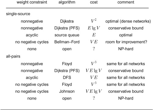
The general problem of finding shortest paths in networks where edge weights could be negative is intractable. Shortest-paths problems are a good illustration of the fine line that often separates intractable problems from easy ones, since we have numerous algorithms to solve the various versions of the problem when we restrict the networks to have positive edge weights or to be acyclic, or even when we restrict to subproblems where there are negative edge weights but no negative cycles. Several of the algorithms are optimal or nearly so, although there are significant gaps between the best known lower bound and the best known algorithm for the single-source problem in networks that contain no negative cycles and for the all-pairs problem in networks that contain nonnegative weights.

The algorithms are all based on a small number of abstract operations and can be cast in a general setting. Specifically, the only operations that we perform on edge weights are addition and comparison: any setting in which these operations make sense can serve as the platform for shortest-paths algorithms. As we have noted, this point of view unifies our algorithms for computing the transitive closure of digraphs with our algorithms for finding shortest paths in networks. The difficulty presented by negative edge weights corresponds to a monotonicity property on these abstract operations: If we can ensure that the sum of two weights is never less than either of the weights, then we can use the algorithms in Sections 21.2 through 21.4; if we cannot make such a guarantee, we have to use the algorithms from Section 21.7. Encapsulating these considerations in an ADT is easily done and expands the utility of the algorithms.

Shortest-paths problems put us at a crossroad, between elementary graph-processing algorithms and problems that we cannot solve. They are the first of several other classes of problems with a similar character that we consider, including network-flow problems and linear programming. As in shortest paths, there is a fine line between easy and intractable problems in those areas. Not only are numerous efficient algorithms available when various restrictions are appropriate, but also there are numerous opportunities where better algorithms have yet to be invented and numerous occasions where we are faced with the certainty of NP-hard problems.

Many such problems were studied in detail as OR problems before the advent of computers or computer algorithms. Historically, OR has focused on general mathematical and algorithmic models, whereas computer science has focused on specific algorithmic solutions and basic abstractions that can both admit efficient implementations and help to build general solutions. As models from OR and basic algorithmic abstractions from computer science have both been applied to develop implementations on computers that can solve huge practical problems, the line between OR and computer science has blurred in some areas: For example, researchers in both fields seek efficient solutions to problems such as shortest-paths problems. As we address more difficult problems, we draw on classical methods from both fields of research.